GEMPACK manual
Mark Horridge, Michael Jerie, Dean Mustakinov, Florian Schiffmann
31 Dec 2024
ISBN 978-1-921654-90-9
This online version of the GEMPACK documentation is designed for effective searching and navigation within your browser. You can click on on any blue link to jump to the indicated place, and use the Back button to return. Use the middle mouse button to open a link in a new tab. A yellow panel is visible at top right, with links to the Contents page and Index. To find information on a particular topic, go to the Index first. You can also use your browser's Edit..Find command to search through the entire document.
You can use your browser's View menu to adjust the text size. Or, using your keyboard, press CTRL and + or CTRL and - to zoom in or out. If your mouse has a wheel, hold down the CTRL key, and then scroll the wheel to zoom in or out. You may need to wait a second or two to see the effect.
This manual refers to GEMPACK Release 12.2 and later — but will be useful too for earlier releases.
Each section or subsection has a "topic ID" which appears in green at the end of section headings. GEMPACK programs may emit warning or error messages that refer you to sections of this manual. The references may include section numbers, section titles and topic IDs, but the topic ID is most likely to remain unchanged through successive revisions of the manual.
If you want to print out sections, use the matching PDF file, GPmanual.pdf.
We thank Ken Pearson and Jill Harrison who wrote large parts of previous GEMPACK manuals; much of their work is incorporated here.
A condition of your GEMPACK licence is that acknowledgement of GEMPACK must be made when reporting results that have been obtained with GEMPACK. To cite this manual, use:
Horridge J.M., Jerie M., Mustakinov D. & Schiffmann F. (2024), GEMPACK manual, GEMPACK Software, Centre of Policy Studies, Victoria University, Melbourne, ISBN 978-1-921654-34-3, https://ideas.repec.org/p/cop/wpaper/gpman.html
Other GEMPACK-related citations are suggested in section 1.7.
Brief Table of Contents
- 1 Introduction [gpd1.1]
- 2 Installing GEMPACK on Windows PCs [gpd6.1]
- 3 How to carry out simulations with models [gpd1.2]
- 4 Building or modifying models [gpd1.3]
- 5 Header Array files [harfiles]
- 6 Constructing HAR files [gpd1.4]
- 7 GEMPACK file types, names and suffixes [gpd1.5.8]
- 8 Overview of running TABLO and the TABLO language [gpd2.1]
- 9 Additional information about running TABLO [gpd2.2]
- 10 The TABLO language: basic syntax [gpd2.3]
- 11 Syntax and semantic details [gpd2.4]
- 12 TABLO statements for post-simulation processing [gpd5.2]
- 13 Ranking sets via data (finding winners and losers) [gpd5.3]
- 14 Condensing models [condense]
- 15 Verifying economic models [gpd2.6]
- 16 Intertemporal models [gpd2.7]
- 17 Less obvious examples of the TABLO language [gpd2.8]
- 18 Linearizing levels equations [gpd2.9]
- 19 Overview of simulation reference chapters 20 to 35 [gpd3.1]
- 20 Command (CMF) files [gpd3.2]
- 21 TABLO input files and auxiliary files [gpd3.3]
- 22 CMF statements for data files, updated data files and display files [gpd3.4]
- 23 Specifying the closure [gpd3.5.1a]
- 24 Specifying the shocks [gpd3.5.5]
- 25 Actions in GEMSIM and TABLO-generated programs [gpd3.6]
- 26 Multi-step solution methods [gpd3.7]
- 27 Solution (SL4) files [gpd3.8]
- 28 SLC, UDC, AVC and CVL files [slcfiles]
- 29 Subtotals via GEMSIM or TABLO-generated programs [gpd3.11]
- 30 Solving models and simulation time [gpd3.12]
- 31 Solving a model in parallel on a machine with two or more processors [gpd9.2]
- 32 Memory management [gpd3.13]
- 33 Options for GEMSIM and TABLO-generated programs [gpd3.14]
- 34 Run-time errors [gpd3.15]
- 35 Summary of command file statements [gpd3.18]
- 36 GEMPACK Windows programs [gpd4.2]
- 37 Command-line programs for working with header array files [gpd4.4]
- 38 Syntax of GEMPACK text data files [gpd4.6]
- 39 SLTOHT: processing simulation results [gpd4.8]
- 40 SLTOHT for spreadsheets [gpd4.9]
- 41 ACCUM and DEVIA : accumulation and differences [gpd4.10]
- 42 Hands-on tutorials for models supplied with GEMPACK [gpd8.1]
- 43 Getting started with GEMPACK via WinGEM [gpd8.2]
- 44 Command prompt: hands-on computing [gpd8.3]
- 45 Using RunGEM for simulations [gpd8.5]
- 46 Using AnalyseGE to analyse simulation results [gpd8.6]
- 47 Print edition ends here [endprint]
- 48 Working with GEMPACK command-line programs [gpd1.5]
- 49 Miscellaneous information [miscstuff]
- 50 Code options when running TABLO [gpd2.5]
- 51 Simulations for models with complementarities [gpd3.16]
- 52 Subtotals with complementarity statements [gpd5.7]
- 53 More examples of post-simulation processing [postsim2]
- 54 Using MODHAR to create or modify header array files [gpd4.3]
- 55 Ordering of variables and equations in solution and equation files [ordering]
- 56 SEENV: to see the closure on an environment file [gpd4.12]
- 57 Automated homogeneity testing [autohomog]
- 58 Several simultaneous Johansen simulations via SAGEM [gpd3.10]
- 59 Equations files and LU files [gpd3.9]
- 60 Example models supplied with GEMPACK [models]
- 61 Pivoting, memory-sharing, and other solution strategies [pivots]
- 62 Limited executable-image size limits [exelimits]
- 63 Some technical details of GEMPACK [technical]
- 64 Rarely used features of GEMPACK programs [legacy]
- 65 Choosing sets of variables interactively [gpd4.17]
- 66 Older ways to choose closure and shocks [oldshkclos]
- 67 Improving your TAB and CMF files [better]
- 68 Shock statements designed for use with RunDynam [rdynshoks]
- 69 GEMPACK on Linux, Unix or Mac OS X [unix]
- 70 TEXTBI : extracting TAB, STI and CMF files from AXT, SL4 and CVL files [gpd4.14]
- 71 History of GEMPACK [oldnewfeat]
- 72 TABLO-generated programs and GEMSIM - timing comparison [gpd8.4]
- 73 Fortran compilers for Source-code GEMPACK [fortrans]
- 74 LTG variants and compiler options [gpd6.7.5a]
- 75 Fine print about header array files [gpd4.5]
- 76 Converting binary files: LF90/F77L3 to/from Intel/LF95/GFortran [gpd4.15]
- 77 Translation between GEMPACK and GAMS data files [gdxhar]
- 78 Recent GEMPACK with older RunGTAP or RunDynam [gpd5.12]
- 79 SUMEQ: information from equations files [gpd4.13]
- 80 Older GEMPACK documents [gemdocs]
- 81 References [references]
- 82 Index [index]
- 83 End of document [docend]
Detailed Table of Contents
- 1 Introduction [gpd1.1]
- 1.1 Organization of this manual [manualoutline]
- 1.2 Using this manual [usingmanual]
- 1.2.1 For experienced GEMPACK users [gpd1.1.5.2]
- 1.2.2 For new GEMPACK users -- getting started [gpd1.1.5.1]
- 1.3 Supported Operating Systems [supportedos]
- 1.4 The GEMPACK programs [gpd9.1.5]
- 1.4.1 The original command-line programs [gpd9.1.5.1]
- 1.4.2 The Windows programs [gpd9.1.5.2]
- 1.4.3 TABLO-generated programs [gpd1.1.7.1]
- 1.5 Models supplied with GEMPACK [gpd1.1.8]
- 1.6 Different versions of GEMPACK and associated licences [gpd1.1.9]
- 1.6.1 Source-code versions and licences [gpd1.1.9.1]
- 1.6.2 Unlimited executable-image version and licence [gpd1.1.9.3]
- 1.6.3 Limited executable-image version and licence [gpd1.1.9.2]
- 1.6.4 Using Exe-image and Source-code GEMPACK together [gpeisc]
- 1.6.5 When is a licence needed [gpd1.1.9.7]
- 1.6.6 Introductory licence [gpd1.1.9.5]
- 1.7 Citing GEMPACK [citinggempack]
- 1.8 Communicating with GEMPACK [gpd1.1.2]
- 1.8.1 GEMPACK web site [gpd1.1.3]
- 1.8.2 GEMPACK-L mailing list [gpd1.1.4]
- 1.9 Training Courses [training]
- 1.10 Acknowledgments [ackintro]
- 2 Installing GEMPACK on Windows PCs [gpd6.1]
- 2.1 Preparing to install GEMPACK [gpd6.2]
- 2.1.1 System requirements [gpd6.2.1]
- 2.1.2 Your GEMPACK licence file [gplic]
- 2.1.3 Where to install [instdir]
- 2.1.4 Notes for IT support [itsupport]
- 2.1.5 [Source-code only] Testing the Fortran installation [gpd6.3.3]
- 2.1.6 Configure Anti-virus programs [antivirus]
- 2.2 Installing GEMPACK [gpd6.4]
- 2.2.1 If a warning appears after installing [pcawarning]
- 2.2.2 [Source-code only] If an error occurs [gpd6.4.1.1]
- 2.2.3 Some GEMPACK licences require activation [activation]
- 2.2.4 GEMPACK licence [gpd6.4.4]
- 2.2.5 Changes to your PATH and Environment [gpd6.4.4a]
- 2.2.6 System environment settings for performance [mathlibperf]
- 2.3 Testing the Installation [gpd6.5]
- 2.4 [Source-code only] Re-Testing the Installation [gpd6.5s]
- 2.5 If you still have problems [witsend]
- 2.6 More simulations to test GEMPACK and WinGEM [gpd6.5.3]
- 2.7 Working with GEMPACK [gpd6.6]
- 2.7.1 New model's directory location [gpd6.6.2]
- 2.7.2 [Source-code only] GEMSIM or TABLO-generated programs ? [gpd6.6.3]
- 2.7.3 Text editor [gpd6.6.4]
- 2.7.4 If you installed in a new directory (not C:\GP) [gpd6.4.3]
- 2.7.5 If a program runs out of memory [gpd6.6.5]
- 2.7.6 Copying GEMPACK programs to other PCs [gpd6.6.9]
- 2.8 Manually setting the PATH and GPDIR [gpd6.4.2]
- 2.8.1 Checking and setting PATH and GPDIR [gpd6.4.2.1]
- 2.8.2 Trouble-shooting environment variables [envvartrouble]
- 2.9 Technical Topics [gpd6.7]
- 2.9.1 [Source-code only] Running BuildGP [gpd6.7.3]
- 2.9.2 File association [gpd6.6.7]
- 2.9.3 Keep and Temporary directories and GEMPACK Windows programs [gpd6.6.8]
- 2.9.4 Installing GEMPACK on a network [gpd6.8]
- 2.9.5 Uninstalling GEMPACK [gpd6.7.6]
- 2.9.6 Finding GEMPACK Version and Release Information [identver]
- 2.1 Preparing to install GEMPACK [gpd6.2]
- 3 How to carry out simulations with models [gpd1.2]
- 3.1 An example simulation with stylized Johansen [gpd1.2.1]
- 3.1.1 Introduction to the stylized Johansen model [gpd1.2.1.1]
- 3.1.2 The simulation [gpd1.2.1.2]
- 3.2 Preparing a directory for model SJ [gpd1.2.4.2]
- 3.3 Using GEMPACK: WinGEM or command prompt? [gpd1.2.3]
- 3.4 Stylized Johansen example simulation [gpd1.2.4]
- 3.4.1 Starting WinGEM [gpd1.2.4.1]
- 3.4.2 Setting the working directory [gpd1.2.4.3]
- 3.4.3 Looking at the data directly using ViewHAR [gpd1.2.4.4]
- 3.5 Implementing and running model SJ [gpd1.impsj]
- 3.5.1 TABLO-generated program or GEMSIM? [gpd1.2.4.5]
- 3.5.2 Source-code method: using a TABLO-generated program [gpd1.2.4.6]
- 3.5.3 Executable-image method: using GEMSIM [gpd1.2.4.7]
- 3.5.4 Step 3 - View the Solution using ViewSOL [gpd1.2.viewsol]
- 3.6 The steps in carrying out a simulation [gpd1.2.5]
- 3.6.1 Steps 1 and 2 using a TABLO-generated program (source-code GEMPACK) [gpd1.2.5.1]
- 3.6.2 Steps 1 and 2 using GEMSIM [gpd1.2.5.2]
- 3.6.3 Other Simulations [gpd1.2.5.othsims]
- 3.7 Interpreting the results [gpd1.2.7]
- 3.8 Specifying a simulation [gpd1.2.8]
- 3.9 The updated data - another result of the simulation [gpd1.2.9]
- 3.10 Preparing tables and graphs for a report [gpd1.2.10]
- 3.10.1 Example 1: Copying from ViewSOL to Spreadsheet and WordProcessor [gpd1.2.viewsolexport]
- 3.10.2 Example 2: Using the GEMPACK Program SLTOHT and Option SSS [gpd1.2.sltoht1]
- 3.10.3 Example 3: Using the Program SLTOHT and Option SES [gpd1.2.sltoht2]
- 3.10.4 Graphs [gpd1.2.10.1]
- 3.11 Changing the closure and shocks [gpd1.2.11]
- 3.12 How Johansen and multi-step solutions are calculated [gpd1.2.13]
- 3.12.1 The linearized equations of a model [gpd1.2.13.1]
- 3.12.2 Johansen solutions [gpd1.2.13.2]
- 3.12.3 Multi-step simulations and accurate solutions of nonlinear equations [gpd1.2.13.3]
- 3.12.4 Smiling or frowning face numbers are reported [gpd5.9.2.1]
- 3.12.5 Fatal error if accuracy too low (GEMSIM and TG-programs) [gpd5.9.2.2]
- 3.13 GEMPACK programs - an overview [gpd1.2.14]
- 3.13.1 Working with TABLO input files [gpd1.2.14.1]
- 3.13.2 Carrying out simulations [gpd1.2.14.2]
- 3.13.3 Looking at, and processing, simulation results [gpd1.2.14.3]
- 3.13.4 Working with data [gpd1.2.14.4]
- 3.13.5 Windows modelling environments [gpd1.2.14.5]
- 3.13.6 Other programs for special tasks [gpd1.2.14.6]
- 3.13.7 Programs for use on non-Windows PCs [gpd1.2.14.7]
- 3.14 Different GEMPACK files [gpd1.2.15]
- 3.14.1 The most important files [gpd1.2.15.1]
- 3.14.2 Files for communication between programs [gpd1.2.15.2]
- 3.14.3 LOG files [gpd1.2.15.3]
- 3.14.4 Stored-input (STI) files [gpd1.2.15.4]
- 3.14.5 Files for power users [gpd1.2.15.5]
- 3.14.6 Summary of files [gpd1.2.15.7]
- 3.14.7 Work files [gpd1.2.15.6]
- 3.14.8 Files you can eventually delete [junkfiles]
- 3.15 For new users - what next? [gpd1.2.16]
- 3.1 An example simulation with stylized Johansen [gpd1.2.1]
- 4 Building or modifying models [gpd1.3]
- 4.1 Writing down the equations of a model [gpd1.3.1]
- 4.2 Data requirements for the linearized equations [gpd1.3.2]
- 4.2.1 Data requirements for Stylized Johansen [gpd1.3.2.1]
- 4.3 Constructing the TABLO input file for a model [gpd1.3.3]
- 4.3.1 Viewing the TABLO input file [gpd1.3.3.1]
- 4.3.2 Constructing part of the TABLO input file for Stylized Johansen [gpd1.3.3.2]
- 4.3.3 "Mixed" TABLO input file for the Stylized Johansen model [gpd1.3.3.3]
- 4.3.4 Completing the TABLO input file for Stylized Johansen [gpd1.3.3.4]
- 4.3.5 Change or percentage-change variables [gpd1.3.3.5]
- 4.3.6 Variable or parameter ? [gpd1.3.3.6]
- 4.3.7 TABLO language - syntax and semantics [gpd1.3.3.7]
- 4.4 Linearized TABLO input files [gpd1.3.4]
- 4.4.1 A linearized TABLO input file for Stylized Johansen [gpd1.3.4.1]
- 4.4.2 Noteworthy features in the linearized TABLO input file [gpd1.3.4.2]
- 4.4.3 Analysing simulation results [gpd1.3.4.3]
- 4.4.4 Writing UPDATE statements [gpd1.3.4.4]
- 4.4.5 Numerical versions of linearized equations [gpd1.3.4.5]
- 4.4.6 Numerical examples of update statements [gpd1.3.4.6]
- 4.4.7 How equations are recalculated in a multi-step calculation [gpd1.3.4.7]
- 4.5 Levels TABLO input files [gpd1.3.5]
- 4.5.1 Levels TABLO input file for Stylized Johansen [gpd1.3.5.1]
- 4.6 TABLO linearizes levels equations automatically [gpd1.3.7]
- 4.7 Creating the TABLO input file and command files for your own model [gpd1.3.9]
- 4.7.1 Correcting errors in TABLO input files [gpd1.3.9.1]
- 4.7.2 Correcting errors in command files [gpd1.3.9.2]
- 5 Header Array files [harfiles]
- 5.0.1 Data on Header Array files [gpd4.3.1]
- 5.0.2 Array type [gpd4.3.1.1]
- 5.0.3 Set and element labelling on header array files [gpd4.5a]
- 5.0.4 Long names [gpd4.3.1.2]
- 5.0.5 File history and creation information [gpd9.7.5.3]
- 5.1 Ways to create or modify header array files [gpd4.3.2]
- 6 Constructing HAR files [gpd1.4]
- 6.1 Constructing the header array data file for Stylized Johansen [sjmkdat]
- 6.2 Editing the header array data file for Stylized Johansen [sjmoddat]
- 6.2.1 Other ViewHAR capabilities [gpd1.4.5.8]
- 6.3 Checking data is balanced [gpd1.4.7]
- 6.3.1 SJCHK.TAB to check balance for Stylized Johansen [gpd1.4.7.1]
- 6.3.2 SJCHK.TAB to check balance of updated data [gpd1.4.7.2]
- 6.3.3 GTAPVIEW for checking and summarising GTAP data [gpd1.4.7.3]
- 6.3.4 Checking the balance of ORANIG data [gpd1.4.7.4]
- 6.4 Which program to use in file conversion? [gpd1.4.8]
- 6.5 Further information [gpd1.4.9]
- 7 GEMPACK file types, names and suffixes [gpd1.5.8]
- 7.0.1 Files with system-determined suffixes [gpd1.5.8.1]
- 7.0.2 Suffixes of other files [gpd1.5.8.2]
- 7.0.3 Files -- binary, header array or text? [gpd1.5.8.3]
- 7.0.4 Why so many files? [gpd1.5.8.4]
- 7.1 Allowed file and directory names [gpd1.5.9]
- 7.1.1 File names containing spaces [gpd1.5.9.4]
- 7.1.2 Characters in stored-input files and command files [gpd1.5.9.5]
- 7.1.3 Files that could be deleted [cleanupfiles]
- 8 Overview of running TABLO and the TABLO language [gpd2.1]
- 8.1 Running TABLO on an existing model [gpd2.1.1]
- 8.1.1 Example models ORANIG01 and GTAP61 [gpd2.1.1.1]
- 8.1.2 TAB file and WFP/PGS on command line [gpd5.10.1.2]
- 8.1.3 Running TABLO from TABmate with no STI file [tablocode]
- 8.1.4 Preliminary pass to count statements [gpd2.1.1.2]
- 8.2 Compiling and linking TABLO-generated programs [gpd2.1.2]
- 8.3 Writing a TABLO input file for a new model [gpd2.1.4]
- 8.4 Modern ways of writing TABLO input files (on a PC) [gpd2.1.5]
- 8.4.1 Using TABmate [gpd2.1.5.1]
- 8.4.2 Using TABmate to find a closure and suggest substitutions [autoclosure]
- 8.4.3 Using TABmate to create a CMF file [autocmf]
- 8.4.4 Using TABmate to reformat your code [beautyparlour]
- 8.4.5 Using ViewHAR to write TABLO code for data manipulation [gpd2.1.5.2]
- 8.5 Condensing a large model [gpd2.1.6]
- 8.5.1 Condensation in STI file: a legacy technique [oldsticond]
- 8.1 Running TABLO on an existing model [gpd2.1.1]
- 9 Additional information about running TABLO [gpd2.2]
- 9.1 TABLO options [gpd2.2.1]
- 9.1.1 TABLO input file written on the auxiliary files [gpd2.2.1.1]
- 9.1.2 TABLO file and TABLO STI file stored on solution file [gpd2.2.1.2]
- 9.1.3 Specialised check options [gpd2.2.1.3]
- 9.1.4 Doing condensation or going to code generation [gpd2.2.1.4]
- 9.1.5 TABLO code options [gpd2.2.1.5]
- 9.1.6 Identifying and correcting syntax and semantic errors [gpd2.2.1.6]
- 9.2 TABLO linearizes levels equations automatically [gpd2.2.2]
- 9.2.1 Change or percentage-change associated linear variables [gpd2.2.2.1]
- 9.2.2 How levels variable statements are converted [gpd2.2.2.2]
- 9.2.3 How levels equation statements are converted [gpd2.2.2.3]
- 9.2.4 Linearizing levels equations [gpd2.2.2.4]
- 9.2.5 Linearizing a sum [gpd2.2.2.5]
- 9.2.6 Algorithm used by TABLO [gpd2.2.2.6]
- 9.2.7 TABLO can write a linearised TAB file [gpd9.7.19]
- 9.3 Reporting Newton error terms in models with levels equations [gpd5.9.14]
- 9.1 TABLO options [gpd2.2.1]
- 10 The TABLO language: basic syntax [gpd2.3]
- 10.1 SET [gpd2.3.1]
- 10.1.1 Set expressions (includes unions, intersections and complements) [gpd2.3.1.0]
- 10.1.2 Equal sets [gpd2.3.1.2]
- 10.1.3 Data-dependent sets [gpd2.3.1.3]
- 10.1.4 Set examples from ORANIG model [gpd2.3.1.5]
- 10.1.5 Set examples from GTAP model [gpd2.3.1.6]
- 10.1.6 Set products [gpd2.3.1.4]
- 10.1.7 Multidimensional sets and tuples [tuples]
- 10.1.8 Ranked sets [gpd2.3.1.6a]
- 10.2 SUBSET [gpd2.3.2]
- 10.2.1 Subset examples from ORANIG model [gpd2.3.2.1]
- 10.2.2 Subset examples from GTAP model [gpd2.3.2.2]
- 10.3 COEFFICIENT [gpd2.3.3]
- 10.4 VARIABLE [gpd2.3.4]
- 10.5 FILE [gpd2.3.5]
- 10.5.1 SSE output [gpd5.9.1]
- 10.6 READ [gpd2.3.6]
- 10.7 WRITE [gpd2.3.7]
- 10.8 FORMULA [gpd2.3.8]
- 10.9 EQUATION [gpd2.3.9]
- 10.9.1 FORMULA & EQUATION [gpd2.3.9.1]
- 10.10 UPDATE [gpd2.3.10]
- 10.11 ZERODIVIDE [gpd2.3.11]
- 10.11.1 More about zerodivides [gpd2.4.13]
- 10.12 DISPLAY [gpd2.3.12]
- 10.13 MAPPING [gpd2.3.13]
- 10.13.1 Formulas for mappings, and reading and writing mappings [gpd2.3.13.1]
- 10.13.2 Projection mappings from a set product [gpd2.3.13.2]
- 10.14 ASSERTION [gpd2.3.14]
- 10.15 TRANSFER [gpd2.3.15]
- 10.16 OMIT, SUBSTITUTE and BACKSOLVE [gpd2.3.16_17_18]
- 10.17 COMPLEMENTARITY [gpd2.3.19]
- 10.18 POSTSIM [gpd2.3.19a]
- 10.19 Setting default values of qualifiers [gpd2.3.20]
- 10.20 TABLO statement qualifiers - a summary [gpd2.3.21]
- 10.20.1 Spaces and qualifier syntax [gpd2.3.21.1]
- 10.1 SET [gpd2.3.1]
- 11 Syntax and semantic details [gpd2.4]
- 11.1 General notes on the TABLO syntax and semantics [gpd2.4.1]
- 11.1.1 TABLO statements [gpd2.4.1.1]
- 11.1.2 Lines of the TABLO input file [gpd2.4.1.2]
- 11.1.3 Upper and lower case [gpd2.4.1.3]
- 11.1.4 Comments [gpd2.4.1.4]
- 11.1.5 Strong comment markers [gpd2.4.1.5]
- 11.1.6 Reserved (special) characters [gpd2.4.1.6]
- 11.1.7 Chinese and accented characters [nonascii]
- 11.2 User defined input [gpd2.4.2]
- 11.2.1 Names [gpd2.4.2.1]
- 11.2.2 Abbreviating lists of set elements [gpd2.4.2.0]
- 11.2.3 Labelling information (text between hashes #) [gpd2.4.2.2]
- 11.2.4 Arguments: indices, set elements or index expressions [gpd2.4.2.3]
- 11.2.5 Index expressions with elements from run-time sets [gpd2.4.2.4]
- 11.3 Quantifiers and quantifier lists [gpd2.4.3]
- 11.4 Expressions used in equations, formulas and updates [gpd2.4.4]
- 11.4.1 Operations used in expressions [gpd2.4.4.1]
- 11.4.2 Brackets in expressions [gpd2.4.4.3]
- 11.4.3 Sums over sets in expressions [gpd2.4.4.2]
- 11.4.4 MaxS, MinS and Prod operators [gpd2.4.4.2a]
- 11.4.5 Conditional quantifiers and SUMs, PRODs, MAXS and MINS [gpd2.4.4.5]
- 11.4.6 Conditional expressions [gpd2.4.4.6]
- 11.4.7 Index-IN-Set condition for IF expressions [gpd2.4.4.6b]
- 11.4.8 Linear variables in expressions [gpd2.4.4.7]
- 11.4.9 Constants in expressions [gpd2.4.4.8]
- 11.4.10 Indices in expressions [gpd2.4.4.9]
- 11.4.11 Index-expression conditions [gpd2.4.4.10]
- 11.5 Functions [gpd2.4.4.4]
- 11.5.1 ID01 and ID0V functions [gpd2.4.4.4.1]
- 11.5.2 RANDOM function [gpd2.4.4.4.2]
- 11.5.3 Statistical functions [statistical]
- 11.5.4 NORMAL and CUMNORMAL functions [gpd2.4.4.4.3]
- 11.5.5 Functions for log-normal distribution [gpd9.7.9]
- 11.5.6 $POS function [gpd2.4.4.4.4]
- 11.5.7 ROUND, TRUNC0 and TRUNCB functions [gpd2.4.4.4.5]
- 11.6 Coefficients and levels variables [gpd2.4.5]
- 11.6.1 Coefficients -- what are they ? [gpd2.4.5.1]
- 11.6.2 Model parameters [gpd2.4.5.2]
- 11.6.3 Integer coefficients in expressions and elsewhere [gpd2.4.5.3]
- 11.6.4 Where coefficients and levels variables can occur [gpd2.4.5.4]
- 11.6.5 Reporting levels values when carrying out simulations [gpd2.4.5.5]
- 11.6.6 How do you see the pre-simulation and post-simulation levels values? [gpd2.4.5.6]
- 11.6.7 Specifying acceptable range of coefficients read or updated [gpd2.4.5.7]
- 11.7 Sets [gpd2.4.6]
- 11.7.1 Set size and set elements [gpd2.4.6.1]
- 11.7.2 Obsolete "maximum size" in SET statements [gpd2.4.6.2]
- 11.7.3 Set unions, intersections and equality [gpd2.4.6.3]
- 11.7.4 Set complements and relative complements [gpd2.4.6.4]
- 11.7.5 Longer set expressions [gpd2.4.6.4b]
- 11.7.6 Sets whose elements depend on data [gpd2.4.6.5]
- 11.7.7 Writing the elements of one set [gpd2.4.6.6]
- 11.7.8 Writing the elements of all (or many) sets [gpd2.4.6.7]
- 11.7.9 Empty sets [gpd2.4.6.8]
- 11.7.10 Reading set elements from a file [gpd2.4.6.9]
- 11.7.11 Creating element names for set products [gpd2.4.6.10]
- 11.8 Subsets [gpd2.4.7]
- 11.9 Mappings between sets [gpd2.4.8]
- 11.9.1 Defining set mapping values [gpd2.4.8.1]
- 11.9.2 Checking values of a mapping [gpd2.4.8.2]
- 11.9.3 Insisting that a set mapping be onto [gpd2.4.8.3]
- 11.9.4 Using set mappings [gpd2.4.8.4]
- 11.9.5 Set Mappings can only be used in index expressions [gpd2.4.8.5]
- 11.9.6 Two or more set mappings in an index expression [gpd2.4.8.6]
- 11.9.7 Set mappings in arguments [gpd2.4.8.7]
- 11.9.8 Set mappings on LHS of a Formula [mapfmlhs]
- 11.9.9 Other semantics for mappings [gpd2.4.8.8]
- 11.9.10 Writing the values of set mappings [gpd2.4.8.9]
- 11.9.11 Reading part of a set mapping BY_ELEMENTS [gpd2.4.8.10]
- 11.9.12 Mapping values can be given by values of other mapping or index [gpd2.4.8.11]
- 11.9.13 Writing a set mapping to a text file [gpd2.4.8.12]
- 11.9.14 Long name when a set mapping is written to a header array file [gpd2.4.8.14]
- 11.9.15 ViewHAR and set mappings [gpd2.4.8.15]
- 11.10 Files [gpd2.4.9]
- 11.10.1 Text files [gpd2.4.9.1]
- 11.11 Reads, writes and displays [gpd2.4.10]
- 11.11.1 How data is associated with coefficients [gpd2.4.10.1]
- 11.11.2 Partial reads, writes and displays [gpd2.4.10.2]
- 11.11.3 Seeing the values of integer coefficients of dimension 3 or higher [gpd5.8.5]
- 11.11.4 FORMULA(INITIAL)s [gpd2.4.10.3]
- 11.11.5 Coefficient initialisation [gpd2.4.10.4]
- 11.11.6 Display files [gpd2.4.10.5]
- 11.11.7 Transferring long names when executing write statements [gpd2.4.10.6]
- 11.11.8 Reads only if header exists -- read qualifier ifheaderexists [gpd5.8.1]
- 11.12 Updates [gpd2.4.11]
- 11.12.1 Purpose of updates [gpd2.4.11.1]
- 11.12.2 Which type of update? [gpd2.4.11.2]
- 11.12.3 What if an initial value is zero ? [gpd2.4.11.3]
- 11.12.4 UPDATE semantics [gpd2.4.11.4]
- 11.12.5 Example 1 of deriving update statements: sum of two flows [gpd2.4.11.5]
- 11.12.6 Example 2 of deriving update statements: powers of taxes [gpd2.4.11.6]
- 11.12.7 Example 3 of deriving update statements: an update (change) statement [gpd2.4.11.7]
- 11.12.8 Writing updated values from FORMULA(INITIAL)s [gpd2.4.11.8]
- 11.13 Transfer statements [gpd2.4.12]
- 11.13.1 XTRANSFER Statements on command files [gpd2.4.12.1]
- 11.14 Complementarity semantics [gpd2.4.14]
- 11.14.1 Condensation and complementarities [gpd2.4.14.1]
- 11.14.2 Linking the complementarity to existing linear variables [gpd2.4.14.2]
- 11.15 The RAS_MATRIX function [gpd9.7.10]
- 11.15.1 The RAS procedure [gpd9.7.10.1]
- 11.15.2 An intuitive way to think of the RAS [gpd9.7.10.2]
- 11.15.3 RAS iterations [gpd9.7.10.3]
- 11.15.4 RAS syntax in TABLO [gpd9.7.10.4]
- 11.15.5 The RAS report [gpd9.7.10.5]
- 11.15.6 Warnings of potential problems [gpd9.7.10.6]
- 11.16 Ordering [gpd2.4.15]
- 11.16.1 Ordering of the input statements [gpd2.4.15.1]
- 11.16.2 Order in which reads, formulas, equations and updates are performed [gpd2.4.15.6]
- 11.17 TABLO input files with no equations [gpd2.4.16]
- 11.18 Loops in TAB files [loop-tab]
- 11.1 General notes on the TABLO syntax and semantics [gpd2.4.1]
- 12 TABLO statements for post-simulation processing [gpd5.2]
- 12.1 Simple examples of PostSim statements [postsimexm]
- 12.2 PostSim TAB file statements, syntax and semantic rules [gpd5.2.5]
- 12.2.1 Statements allowed in post-simulation sections of a TAB file [gpd5.2.5.1]
- 12.2.2 Syntax and semantics for formulas in PostSim part of TAB file [gpd5.2.5.2]
- 12.2.3 Semantics for reads in PostSim part of TAB file [gpd5.2.5.3]
- 12.2.4 Semantics for assertions in PostSim part of TAB file [gpd5.2.5.4]
- 12.2.5 Semantics for zerodivides in PostSim part of TAB file [gpd5.2.5.5]
- 12.2.6 Default statements and certain qualifiers not relevant in PostSim part [gpd5.2.5.6]
- 12.2.7 PostSim sets, subsets, coefficients not allowed in the ordinary part [gpd5.2.5.7]
- 12.2.8 PostSim qualifier for write or display [gpd5.2.5.8]
- 12.2.9 Implications for condensation [gpd5.2.5.9]
- 12.3 PostSim extra statements in a command file [gpd5.2.6]
- 12.4 PostSim parts of TAB file and AnalyseGE [gpd5.2.9]
- 12.4.1 Coefficients or expressions selected from the TABmate form [gpd5.2.9.1]
- 12.4.2 Expressions evaluated from the AnalyseGE form [gpd5.2.9.2]
- 12.4.3 UDC files now redundant? [gpd5.2.9.3]
- 12.5 Technical details: When and how is post-simulation part done? [gpd5.2.8]
- 12.6 Advantages of PostSim processing in TAB file [gpd5.2.4]
- 13 Ranking sets via data (finding winners and losers) [gpd5.3]
- 13.1 Example: identifying winners and/or losers [gpd5.3.1]
- 13.1.1 Ranking example OG01PS.TAB [gpd5.3.1.1]
- 13.2 Ranked set statements -- syntax and semantics [gpd5.3.2]
- 13.3 Converting non-intertemporal sets to intertemporal sets and vice versa [gpd5.3.3]
- 13.3.1 TABLO statements [gpd5.3.3.1]
- 13.3.2 Household income example in detail [gpd5.3.3.2]
- 13.1 Example: identifying winners and/or losers [gpd5.3.1]
- 14 Condensing models [condense]
- 14.1 Condensing models [gpd1.3.8]
- 14.1.1 Substituting out variables [gpd1.3.8.1]
- 14.1.2 Condensation examples [gpd1.3.8.2]
- 14.1.3 Backsolving for variables [gpd1.3.8.3]
- 14.1.4 Condensation examples using backsolving [gpd1.3.8.4]
- 14.1.5 Results on the solution file in condensation examples [gpd1.3.8.5]
- 14.1.6 Should all substitutions be backsolves? [gpd1.3.8.6]
- 14.1.7 Omitting variables [gpd1.3.8.7]
- 14.1.8 Automatic substitutions [gpd1.3.8.7b]
- 14.1.9 Condensation actions can be put on the TABLO input file [gpd1.3.8.8]
- 14.1.10 More details about condensation and substituting variables [gpd2.2.3]
- 14.1.11 Looking ahead to substitution when creating TABLO input files [gpd2.2.3.1]
- 14.1.12 System-initiated formulas and backsolves [gpd2.2.3.2]
- 14.1.13 Treating substitutions as backsolves - option ASB [gpd2.2.3.4]
- 14.1.14 Condensation statements on a TABLO input file [gpd2.2.4]
- 14.1.15 Ignoring TABLO condensation [gpd2.2.4.1]
- 14.1.16 Condensation information file [gpd9.7.8]
- 14.1.17 Submatrix nonzeros information file [smnzinffile]
- 14.1.18 CondOpt tool to find optimal condensation [condopt]
- 14.1 Condensing models [gpd1.3.8]
- 15 Verifying economic models [gpd2.6]
- 15.1 Is balanced data still balanced after updating? [gpd2.6.1]
- 15.1.1 Balance after n-steps [gpd2.6.1.1]
- 15.1 Is balanced data still balanced after updating? [gpd2.6.1]
- 16 Intertemporal models [gpd2.7]
- 16.1 Introduction to intertemporal models [gpd2.7.1]
- 16.2 Intertemporal sets [gpd2.7.2]
- 16.3 Use an INTEGER coefficient to count years [gpd2.7.3]
- 16.4 Enhancements to semantics for intertemporal models [gpd2.7.4]
- 16.5 Recursive formulas over intertemporal sets [gpd2.7.5]
- 16.6 Constructing an intertemporal data set satisfying all model equations [gpd2.7.6]
- 16.6.1 Example using the CRTS intertemporal model [gpd2.7.6.1]
- 16.7 ORANI-INT: A multi-sector rational expectations model [gpd2.7.7]
- 17 Less obvious examples of the TABLO language [gpd2.8]
- 17.1 Flexible formula for the size of a set [gpd2.8.1]
- 17.2 Adding across time periods in an intertemporal model [gpd2.8.2]
- 17.3 Conditional functions or equations [gpd2.8.3]
- 17.3.1 Other methods [gpd2.8.3b]
- 17.4 Aggregating data and simulation results [gpd2.8.4]
- 17.5 Use of special sets and coefficients [gpd2.8.5]
- 18 Linearizing levels equations [gpd2.9]
- 18.1 Differentiation rules used by TABLO [gpd2.9.1]
- 18.2 Linearizing equations by hand [gpd2.9.2]
- 18.2.1 General procedure - change differentiation [gpd2.9.2.1]
- 18.2.2 Rules to use [gpd2.9.2.2]
- 18.2.3 Linearizing equations in practice [gpd2.9.2.3]
- 18.2.4 Linearizing using standard references [gpd2.9.2.4]
- 18.3 Linearized equations on information file [gpd2.9.3]
- 18.4 Linearized equations via AnalyseGE [gpd2.9.3b]
- 18.5 Be careful when using linearized equations [gpd2.9.4]
- 18.6 Keep formulas and equations in synch [gpd2.9.4b]
- 19 Overview of simulation reference chapters 20 to 35 [gpd3.1]
- 20 Command (CMF) files [gpd3.2]
- 20.1 Data manipulation using GEMSIM or TABLO-generated programs [gpd3.2.2]
- 20.2 Simulations using GEMSIM or TABLO-generated programs [gpd3.2.1]
- 20.3 SAGEM simulations [gpd3.2.3]
- 20.4 File names [gpd3.2.4]
- 20.4.1 Naming the command file [gpd3.2.4.1]
- 20.4.2 File names containing spaces [gpd3.2.4.2]
- 20.5 Using the command file stem for names of other output files [gpd3.2.5]
- 20.5.1 Default: solution file stem = command file stem [gpd3.2.5.1]
- 20.5.2 Default: log file stem = command file stem [gpd3.2.5.2]
- 20.5.3 Default: display file stem = command file stem [gpd3.2.5.3]
- 20.5.4 Using <CMF> in command files [gpd3.2.5.4]
- 20.5.5 Position of <CMF> in command file statements [gpd9.7.16]
- 20.6 Log files and reporting CPU time [gpd3.2.6]
- 20.7 General points about command file statements [gpd3.2.7]
- 20.8 Eliminating syntax errors in GEMPACK command files [gpd3.2.8]
- 20.9 Replaceable parameters in CMF files [cmfparm]
- 20.9.1 The newcmf= option [newcmf]
- 21 TABLO input files and auxiliary files [gpd3.3]
- 21.1 GEMSIM and GEMSIM auxiliary files [gpd3.3.1]
- 21.2 TABLO-generated programs and auxiliary files [gpd3.3.2]
- 21.3 How are the names of the auxiliary files determined? [gpd3.3.3]
- 21.4 Check that auxiliary files are correct [gpd3.3.4]
- 21.4.1 Model information (MIN) file date [gpd3.3.4.1]
- 21.5 Carrying out simulations on other machines [gpd3.3.5]
- 21.5.1 Copying TABLO-generated programs to other PCs [gpd3.3.5.1]
- 21.5.2 GEMPACK licence may be required [gpd3.3.5.2]
- 22 CMF statements for data files, updated data files and display files [gpd3.4]
- 22.1 Data files and logical files [gpd3.4.1]
- 22.1.1 Input and output data files [gpd3.4.1.1]
- 22.1.2 Using the same filename twice in CMF files [dupefilenames]
- 22.2 Updated data files [gpd3.4.2]
- 22.2.1 Naming updated files [gpd3.4.2.1]
- 22.2.2 Updated data read from the terminal [gpd3.4.2.2]
- 22.2.3 Intermediate data files [gpd3.4.2.3]
- 22.2.4 Long names on updated data files [gpd3.4.2.4]
- 22.3 Display files [gpd3.4.3]
- 22.3.1 Options for display files [gpd3.4.3.1]
- 22.4 Checking set and element information when reading data [gpd3.4.4]
- 22.5 Names of intermediate data files [gpd3.4.5]
- 22.1 Data files and logical files [gpd3.4.1]
- 23 Specifying the closure [gpd3.5.1a]
- 23.1 The closure [gpd3.5.1]
- 23.1.1 Miniature ORANI model [gpd3.5.1.1]
- 23.2 Specifying the closure via a command file [gpd3.5.2]
- 23.2.1 Listing exogenous variable names and components. [gpd3.5.2.1]
- 23.2.2 Closure swap statements [gpd3.5.2.1a]
- 23.2.3 Order of command file statements can be important [gpd3.5.2.4]
- 23.2.4 Closure specified using data files [gpd3.5.2.5]
- 23.2.5 Using a saved closure [gpd3.5.2.2]
- 23.2.6 List of exogenous/endogenous variables when closure is invalid [gpd3.5.2.6]
- 23.2.7 Initial closure check and singular matrices [gpd3.5.2.7]
- 23.1 The closure [gpd3.5.1]
- 24 Specifying the shocks [gpd3.5.5]
- 24.1 Specifying simple shocks [gpd3.5.5.1]
- 24.2 Reading nonuniform shocks from a file [gpd3.5.5.2]
- 24.3 Using the "select from" shock statement [gpd3.5.5.1b]
- 24.4 Shock components must usually be in increasing order [gpd3.5.5.3]
- 24.5 When to use "select from" [gpd9.7.17]
- 24.6 Other points about shocks [gpd3.5.5.4x]
- 24.6.1 Using SEENV to generate shock statements [gpd3.5.5.4seenv]
- 24.6.2 Shock statements using component numbers and/or lists of values [gpd3.5.5.4b]
- 24.6.3 Shocking a variable with no components exogenous [gpd3.5.5.5]
- 24.7 FINAL_LEVEL statements : alternatives to shock statements [gpd3.5.6]
- 24.8 Shocks from a coefficient [shcoeff]
- 24.8.1 Examples [shcoeff1]
- 24.8.2 Motivation [shcoeff2]
- 24.8.3 Formal rules [shcoeff3]
- 24.8.4 Fine print [shcoeff4]
- 24.9 CHANGE or PERCENT_CHANGE shock statements [gpd3.5.7]
- 24.10 Rate% shock statement [gpd5.9.16]
- 24.10.1 Fine print about rate% shock statements [gpd5.9.16.1]
- 24.11 Shock files: fine print [gpd3.5.8b]
- 24.12 Checking the closure and shocks [gpd3.5.9]
- 24.13 Levels variable names can be used in command files [gpd3.5.10]
- 24.14 Clarification concerning shocks on a command file [gpd3.5.11]
- 24.14.1 Shock statement when only some components are exogenous [gpd3.5.11.1]
- 24.14.2 At least one shock statement is required. [gpd3.5.11.2]
- 25 Actions in GEMSIM and TABLO-generated programs [gpd3.6]
- 25.1 Possible actions in GEMSIM and TABLO-generated programs [gpd3.6.1]
- 25.1.1 Multi-step simulations with economic models [gpd3.6.1.1]
- 25.1.2 Creating an equations file [gpd3.6.1.2]
- 25.1.3 Other actions [gpd3.6.1.3]
- 25.1.4 Data manipulation [gpd3.6.1.4]
- 25.1.5 "extra" (TABLO-like) actions [gpd3.6.1.5]
- 25.1.6 Checking the closure and shocks [gpd3.6.1.6]
- 25.1.7 Postsim passes and actions [gpd3.6.1.6a]
- 25.1.8 Controlling whether and how the actions are carried out [gpd3.6.1.7]
- 25.1.9 Some reads and FORMULAS may be omitted [gpd3.6.1.8]
- 25.1.10 Writes and displays at all steps of a multi-step simulation [gpd3.6.1.9]
- 25.1.11 Echoing activity [gpd3.6.1.10]
- 25.1.12 Writes to the terminal [gpd3.6.1.11]
- 25.2 How these programs carry out multi-step simulations [gpd3.6.2]
- 25.2.1 Processing the closure and shocks [gpd3.6.2.1]
- 25.2.2 Results of a 4-step simulation looked at in detail [gpd3.6.2.2]
- 25.2.3 Do the accurate results satify the linear equations? [gpd3.6.2.3]
- 25.3 Assertions [gpd3.6.3]
- 25.4 Range tests [gpd3.6.4]
- 25.4.1 Specifying the allowed range for a coefficient or levels variable [gpd3.6.4.1]
- 25.4.2 Tests carried out [gpd3.6.4.2]
- 25.4.3 An example [gpd3.6.4.3]
- 25.4.4 Associated statements in command files [gpd3.6.4.4]
- 25.5 Transfer statements [gpd3.6.5]
- 25.6 TABLO-like statements in command files [gpd3.6.6]
- 25.6.1 TABLO-like checks of extra statements [gpd3.6.6.1]
- 25.6.2 Qualifiers [gpd3.6.6.2]
- 25.6.3 Other points [gpd3.6.6.3]
- 25.7 Coefficients are fully initialised by default [gpd3.6.7]
- 25.8 How accurate are arithmetic calculations? [gpd3.6.8]
- 25.8.1 Example 1 - GTAPVIEW [gpd3.6.8.1]
- 25.8.2 Example 2 - checking balance of ORANIG data [gpd3.6.8.2]
- 25.1 Possible actions in GEMSIM and TABLO-generated programs [gpd3.6.1]
- 26 Multi-step solution methods [gpd3.7]
- 26.1 What method and how many steps to use ? [gpd3.7.1]
- 26.1.1 Example - GTAP liberalization simulation [gpd3.7.1.1]
- 26.1.2 Command file statements for method and steps [gpd3.7.1.2]
- 26.2 Extrapolation accuracy summaries and files [gpd3.7.2]
- 26.2.1 Accuracy estimates and summaries for variables [gpd3.7.2.1]
- 26.2.2 Accuracy estimates and summaries for updated data [gpd3.7.2.2]
- 26.2.3 Extrapolation accuracy files [gpd3.7.2.3]
- 26.2.4 Accuracy summary information is on solution file [gpd5.9.11]
- 26.2.5 Fine print on how extrapolation is done [gpd5.9.10]
- 26.2.6 Command file statements affecting extrapolation accuracy reports [gpd3.7.2.4]
- 26.3 Splitting a simulation into several subintervals [gpd3.7.3]
- 26.4 Automatic accuracy for simulations [gpd3.7.4]
- 26.4.1 Specifying which solutions to use [gpd3.7.4.1]
- 26.4.2 Incompatibilities [gpd3.7.4.2]
- 26.4.3 Adaptive stepsize method [gpd3.7.4.4]
- 26.4.4 Stopping if subintervals become too small [gpd3.7.4.5]
- 26.4.5 Controlling which values are tested [gpd3.7.4.6]
- 26.4.6 Checking progress during a run [gpd3.7.4.7]
- 26.5 Runge-Kutta solution methods [rungekutta]
- 26.5.1 Adaptive stepsize for Runge-Kutta [adaptiverk]
- 26.5.2 Which RK integrator to choose? [whichrk]
- 26.6 Newton's method for levels models [gpd3.7.5]
- 26.6.1 Newton's method and ORANIF [gpd3.7.5.1]
- 26.6.2 Convergence [gpd3.7.5.2]
- 26.6.3 General advice [gpd3.7.5.3]
- 26.6.4 Newton's method is not reliable with mixed models [gpd3.7.5.4]
- 26.6.5 Command file statements for Newton's method [gpd5.9.13]
- 26.7 Homotopy methods and levels equations [gpd3.7.6]
- 26.7.1 Example 1 - solving a system of levels equations [gpd3.7.6.1]
- 26.7.2 Example 2 - finding an intertemporal data set [gpd3.7.6.2]
- 26.7.3 Example 3 - use when adding behaviour to a model [gpd3.7.6.3]
- 26.7.4 Formal documentation about ADD_HOMOTOPY [gpd3.7.6.4]
- 26.7.5 Names for homotopy variables added to levels equations [gpd5.8.6]
- 26.7.6 ADD_HOMOTOPY and NOT_ADD_HOMOTOPY default statements [gpd3.7.6.5]
- 26.8 Options for saving solution and updated data files [gpd3.7.7]
- 26.9 Solutions report perturbations of the initial values [gpd3.7.8]
- 26.9.1 Change differentiation keeps a constant error [gpd3.7.8.1]
- 26.9.2 How can homotopies help? [gpd3.7.8.2]
- 26.1 What method and how many steps to use ? [gpd3.7.1]
- 27 Solution (SL4) files [gpd3.8]
- 27.1 Command file statements related to solution files [gpd3.8.1]
- 27.2 Contents of solution files [gpd3.8.2]
- 27.2.1 TAB and STI files stored on solution file [gpd3.8.2.1]
- 27.2.2 Command file stored on solution file [gpd3.8.2.2]
- 27.3 Displaying Levels results [gpd3.8.3]
- 27.4 SEQ files [seqfiles]
- 28 SLC, UDC, AVC and CVL files [slcfiles]
- 29 Subtotals via GEMSIM or TABLO-generated programs [gpd3.11]
- 29.1 Subtotals from GEMSIM and TABLO-generated programs [gpd3.11.1]
- 29.2 Meaning of subtotals results [gpd3.11.2]
- 29.3 Subtotal example [gpd3.11.3]
- 29.4 More substantial examples [gpd3.11.4]
- 29.5 Processing subtotal results [gpd3.11.5]
- 29.6 Subtotals results depend on the path [gpd3.11.6]
- 30 Solving models and simulation time [gpd3.12]
- 30.1 How GEMPACK programs solve linear equations [gpd3.12.1]
- 30.1.1 GEMPACK 12 LU factorization [gp12lu]
- 30.1.2 Sparse-linear-equation solving routines MA48 and MA28 [gpd3.12.1.1]
- 30.1.3 Which to use? MA48 or MA28 [gpd3.12.1.2]
- 30.1.4 Accuracy warnings from iterative refinement [gpd9.7.6]
- 30.1.5 Iterative refinement and residual ratios [itref2]
- 30.2 Gragg's method and the midpoint method [gpd3.12.2]
- 30.3 Reusing pivots [gpd3.12.3]
- 30.4 Ignoring/keeping zero coefficients [gpd3.12.5]
- 30.4.1 More details about the "iz1=no" option [gpd3.12.5a]
- 30.5 LU decomposition [gpd5.5]
- 30.6 Equation solving problems [gpd3.12.6]
- 30.7 Work files [gpd3.12.7]
- 30.1 How GEMPACK programs solve linear equations [gpd3.12.1]
- 31 Solving a model in parallel on a machine with two or more processors [gpd9.2]
- 31.1 You need plenty of memory [gpd9.2.1]
- 31.2 Telling the program to run in parallel [gpd9.2.2]
- 31.3 Restrictions [gpd9.2.3]
- 31.4 Servants work in their own directories [gpd9.2.4]
- 31.5 Master log file is complete [gpd9.2.5]
- 31.6 When the servants start and finish [gpd9.2.6]
- 31.6.1 If there are several subintervals [gpd9.2.6.1]
- 31.6.2 If there are complementarity statements [gpd9.2.6.2]
- 31.6.3 If using automatic accuracy [gpd9.2.6.3]
- 31.7 If a fatal error occurs [gpd9.2.7]
- 31.8 Fine print [gpd9.2.8]
- 31.9 Some elapsed times [gpd9.2.9]
- 31.9.1 Comments on the elapsed times reported [gpd9.2.9.1]
- 31.10 Using master/servant under RunDynam [gpd9.2.10]
- 32 Memory management [gpd3.13]
- 32.1 Automatic memory allocation [gpd3.13.1]
- 32.2 Preliminary pass [gpd3.13.2]
- 32.3 MMNZ: Allocating memory for the LU decomposition [gpd3.13.3]
- 32.4 Reporting memory used by TABLO-generated programs and GEMSIM [gpd3.13.4]
- 32.4.1 RunDynam manages MMNZ start values [rundynam.mmnz]
- 32.4.2 TGMEM1 and TGMEM2 parts of memory [gpd3.13.4.1]
- 33 Options for GEMSIM and TABLO-generated programs [gpd3.14]
- 33.1 Options affecting simulations [gpd3.14.1]
- 33.2 Options affecting extrapolation accuracy summaries and files [gpd3.14.2]
- 33.3 Saving updated values from all FORMULA(INITIAL)s [gpd3.14.3]
- 33.4 Options affecting the actions carried out [gpd3.14.4]
- 33.5 Options affecting how writes and displays are carried out [gpd3.14.5]
- 33.6 Options affecting CPU and activity reporting [gpd3.14.6]
- 33.7 Special options for SAGEM [gpd3.14.7]
- 33.7.1 SAGEM options [gpd3.14.7.1]
- 34 Run-time errors [gpd3.15]
- 34.1 Simulation fails because of a singular LHS matrix [gpd3.15.1]
- 34.1.1 Trying to fix a singular matrix problem [gpd3.15.1.1]
- 34.2 Structurally singular matrices [gpd3.15.2]
- 34.3 Reporting arithmetic errors [gpd9.7.4]
- 34.3.1 Updates -- fine print [gpd9.7.4.1]
- 34.3.2 Other arithmetic errors [gpd9.7.4.2]
- 34.4 Suppressing arithmetic errors in GEMSIM and TABLO-generated programs [gpd5.9.15]
- 34.1 Simulation fails because of a singular LHS matrix [gpd3.15.1]
- 35 Summary of command file statements [gpd3.18]
- 35.1 Command files for GEMSIM and TABLO-generated programs [gpd3.18.1]
- 35.2 Command file statements [gpd3.18.2]
- 35.2.1 Method and steps [gpd3.18.2.1]
- 35.2.2 Checking set and element labelling when reading data from HAR files [gpd3.18.2.2]
- 35.2.3 Checking element names when reading sets from HAR files [gpd3.18.2.3]
- 35.2.4 Automatic accuracy [gpd3.18.2.4]
- 35.2.5 Data files [gpd3.18.2.5]
- 35.2.6 Equations files and BCV files [gpd3.18.2.6]
- 35.2.7 Other files [gpd3.18.2.7]
- 35.2.8 TABLO-like statements in command files [gpd3.18.2.8]
- 35.2.9 Closure related [gpd3.18.2.9]
- 35.2.10 Harwell parameter [gpd3.18.2.10]
- 35.2.11 Verbal description [gpd3.18.2.11]
- 35.2.12 Shock related [gpd3.18.2.12]
- 35.2.13 Cumulatively-retained rows [gpd3.18.2.13]
- 35.2.14 Variables on extrapolation accuracy file [gpd3.18.2.14]
- 35.2.15 Subtotals [gpd3.18.2.15]
- 35.2.16 Complementarity [gpd3.18.2.16]
- 35.2.17 LU decomposition and advanced use of pivots [cmfsum.pivots]
- 35.2.18 Newton's Method [cmfsum.newton]
- 35.2.19 Memory management [cmfsum.sharemem]
- 35.2.20 GEMSIM and TABLO-generated program options [gpd3.18.2.17]
- 35.2.21 Automatic Homogeneity Testing [cmfautohomog]
- 35.2.22 For debugging [gpd3.18.2.18]
- 35.2.23 General points [gpd3.18.2.19]
- 35.3 Complete command file example for GEMSIM and TABLO-generated programs [gpd3.18.3]
- 35.4 Command files for SAGEM [gpd3.18.4]
- 35.5 Command file statements for SAGEM [sagem.cmfs]
- 35.5.1 Equations file, Solution file and Harwell Parameter [gpd3.18.4.1]
- 35.5.2 Verbal description (mandatory) [gpd3.18.4.2]
- 35.5.3 Closure related [gpd3.18.4.3]
- 35.5.4 Shock related [gpd3.18.4.4]
- 35.5.5 Individually-retained and cumulatively-retained rows/columns [gpd3.18.4.5]
- 35.5.6 Subtotals [gpd3.18.4.6]
- 35.5.7 SAGEM options [gpd3.18.4.7]
- 35.5.8 General points [gpd3.18.4.8]
- 35.6 Complete command file example for SAGEM [gpd3.18.5]
- 36 GEMPACK Windows programs [gpd4.2]
- 36.1 WinGEM -- the Windows interface to GEMPACK [gpd4.2.1]
- 36.2 ViewHAR for looking at or modifying data on a header array file [gpd4.2.2]
- 36.2.1 The Charter [gpd4.2.2.1]
- 36.3 ViewSOL for looking at simulation results on a solution file [gpd4.2.3]
- 36.4 TABmate for working on TABLO input files or command files [gpd4.2.4]
- 36.5 RunGEM for model users [gpd4.2.5]
- 36.5.1 TABmate and RunGEM for model developers? [gpd4.2.5.1]
- 36.5.2 Preparing a model for use with RunGEM [gpd4.2.5.2]
- 36.5.3 Systematic sensitivity analysis via RunGEM [gpd4.2.5.3]
- 36.5.4 Systematic sensitivity analysis [gpd4.2.5.4]
- 36.6 AnalyseGE -- assisting in the analysis of simulation results [gpd4.2.6]
- 36.6.1 Using AnalyseGE with data manipulation TAB files [gpd4.2.6.1]
- 36.6.2 Using AnalyseGE when a simulation crashes [gpd4.2.6.2]
- 36.6.3 Subtotals in AnalyseGE [gpd5.6.1]
- 36.6.4 Decomposing selected expression [gpd5.6.2]
- 36.6.5 Analysing closure problems with AnalyseGE [anal-clos]
- 36.7 RunDynam for recursive dynamic models [gpd4.2.7]
- 37 Command-line programs for working with header array files [gpd4.4]
- 37.1 SEEHAR: prepare a print file or CSV spreadsheet file [gpd4.4.1]
- 37.1.1 SEEHAR - options [gpd4.4.1.1]
- 37.1.2 Displays and labelled output from SEEHAR into spreadsheets [gpd4.4.1.2]
- 37.1.3 GAMS output from SEEHAR, TABLO-generated programs and GEMSIM [gpd4.4.1.3]
- 37.1.4 Converting header array files to data bases - SEEHAR option SQL [gpd4.4.1.4]
- 37.1.5 SEEHAR command-line options [seehar12]
- 37.2 CMPHAR: comparing data on header array files [gpd4.4.2]
- 37.2.1 CMPHAR report [gpd4.4.2.1]
- 37.2.2 Significant differences [gpd4.4.2.2]
- 37.2.3 Comparing solution files [gpd4.4.2.3]
- 37.2.4 CMPHAR files on the command line [gpd5.10.1.4]
- 37.2.5 CMPHAR reports difference metric values [gpd5.10.5]
- 37.3 CMBHAR: combining similar header array files [gpd4.4.4]
- 37.4 SUMHAR: summarising a header array file [gpd4.4.3]
- 37.4.1 SUMHAR command-line options [sumhar12]
- 37.5 MergeHAR: combining headers from two HAR files into one [mergehar]
- 37.6 DiffHAR: compare two header or SL4 files [diffhar]
- 37.7 DumpSets: extract sets from HAR file [dumpsets]
- 37.1 SEEHAR: prepare a print file or CSV spreadsheet file [gpd4.4.1]
- 38 Syntax of GEMPACK text data files [gpd4.6]
- 38.1 The "how much data" information [gpd4.6.1]
- 38.1.1 Real or integer data [gpd4.6.1.1]
- 38.1.2 Examples of "how much data" information [gpd4.6.1.2]
- 38.1.3 Character string data [gpd4.6.1.3]
- 38.1.4 Header and longname [gpd4.6.1.4]
- 38.1.5 Coefficient [gpd4.6.1.5]
- 38.1.6 Comments [gpd4.6.1.6]
- 38.1.7 Complete example of GEMPACK text data file [gpd4.6.1.7]
- 38.2 Data values in text files [gpd4.6.2]
- 38.2.1 Array sizes [gpd4.6.2.1]
- 38.2.2 Actual data values of the array [gpd4.6.2.2]
- 38.2.3 Row order [gpd4.6.2.3]
- 38.2.4 Column order [gpd4.6.2.4]
- 38.2.5 Spreadsheet order [gpd4.6.2.5]
- 38.2.6 Real numbers [gpd4.6.2.6]
- 38.2.7 Repeated values in arrays [gpd4.6.2.7]
- 38.2.8 Character strings [gpd4.6.2.8]
- 38.2.9 Multi-dimensional real arrays [gpd4.6.2.9]
- 38.2.10 Maximum length of lines of a file [gpd4.6.2.10]
- 38.2.11 Differences between row order and spreadsheet style data [gpd4.6.2.11]
- 38.2.12 Text editors and text files [gpd4.6.2.12]
- 38.2.13 Advice for CSV files [gpd4.6.2.13]
- 38.2.14 Element name/number labels [gpd4.6.2.14]
- 38.3 Using TABLO to read, manipulate, and write HAR or text files [gpd1.4.4]
- 38.1 The "how much data" information [gpd4.6.1]
- 39 SLTOHT: processing simulation results [gpd4.8]
- 39.1 Introducing SLTOHT [gpd4.8.1]
- 39.1.1 Ways to run SLTOHT [runningsltoht]
- 39.2 Using SLTOHT to make a HAR file [sltohthar]
- 39.3 Mapping files [gpd4.8.3]
- 39.3.1 Header mapping file [gpd4.8.6.1]
- 39.4 Running SLTOHT from the command line [gpd5.10.1.3]
- 39.5 Running SLTOHT interactively [gpd4.8.4]
- 39.5.1 Choosing solutions for output [gpd4.8.4.1]
- 39.6 Undefined solution values [gpd4.8.4.2]
- 39.7 Levels results - options NLV, LV and SHL [gpd4.8.5]
- 39.8 How SLTOHT arranges several solutions in HAR file output [gpd4.8.6]
- 39.9 GEMPACK text data file output using options SIR, SIC or SS [gpd4.8.7]
- 39.10 Other SLTOHT options [gpd4.8.9]
- 39.10.1 SLTOHT option VAI: variable arguments ignored in HAR output [gpd4.8.6.2]
- 39.10.2 SLTOHT option NEL [gpd4.8.9nel]
- 39.10.3 SLTOHT option SEP [gpd4.8.9sep]
- 39.10.4 SLTOHT option HSS: produce both HAR and spreadsheet outputs [gpd4.8.9hss]
- 39.10.5 SLTOHT option SHK: shock CMF output [gpd4.8.8]
- 39.10.6 SLTOHT option DES [gpd4.8.9des]
- 39.1 Introducing SLTOHT [gpd4.8.1]
- 40 SLTOHT for spreadsheets [gpd4.9]
- 40.1 Spreadsheet mapping files [gpd4.9.1]
- 40.1.1 Example of a spreadsheet mapping file (option SSS) [gpd4.8.3.1]
- 40.1.2 Syntax rules for spreadsheet mapping files [gpd4.9.1.1]
- 40.2 Options spreadsheet (SS) and short spreadsheet (SSS) [gpd4.9.2]
- 40.3 Output of tables using options SES or SSE [gpd4.9.3]
- 40.3.1 Output of levels results using option SES [gpd4.9.3.1]
- 40.3.2 Three and higher dimensional arrays of results [gpd4.9.3.2]
- 40.4 Side-by-side results (SES, SS, SSS or SSE output) [gpd4.9.4]
- 40.5 Tables suitable for producing graphs [gpd4.9.5]
- 40.1 Spreadsheet mapping files [gpd4.9.1]
- 41 ACCUM and DEVIA : accumulation and differences [gpd4.10]
- 41.1 Use with dynamic forecasting models [gpd4.10.1]
- 41.2 ACCUM [gpd4.10.2]
- 41.2.1 Columns showing totals and averages [gpd4.10.2.1]
- 41.2.2 Year-on-year results or accumulated results (option ACC) [gpd4.10.2.2]
- 41.2.3 Accumulated indexes (option ACI) [gpd4.10.2.3]
- 41.2.4 Handling subtotals results in ACCUM [gpd4.10.2.4]
- 41.3 Using DEVIA to prepare a spreadsheet table for the differences [gpd4.10.3]
- 41.3.1 Making sure DEVIA knows change/percent-change variables (option SOL) [gpd4.10.3.1]
- 41.3.2 Year-on-year differences (option NAC) [gpd4.10.3.2]
- 41.3.3 Subtotals results in DEVIA [gpd4.10.3.3]
- 41.3.4 Do subtotals for policy shocks add up to the policy deviation? [dyndevsubtot]
- 41.4 Suppressing arithmetic errors in ACCUM, DEVIA and CMBHAR [gpd5.10.3]
- 42 Hands-on tutorials for models supplied with GEMPACK [gpd8.1]
- 42.1 Overview of chapters 43 to 46 [gpd8.1b]
- 43 Getting started with GEMPACK via WinGEM [gpd8.2]
- 43.1 GEMPACK examples for new users [gpd8.2.1]
- 43.2 Locating the example files [gpd8.2.2]
- 43.2.1 Editing text files in WinGEM [gpd8.2.2.1]
- 43.3 Examples using the Stylized Johansen model SJ [gpd8.2.4]
- 43.3.1 Starting WinGEM [gpd8.2.4.1]
- 43.3.2 Preparing a directory for model SJ [gpd8.2.4.2]
- 43.3.3 Setting the working directory [gpd8.2.4.3]
- 43.3.4 Looking at the data directly using ViewHAR [gpd8.2.4.4]
- 43.3.5 TABLO-generated program or GEMSIM? [gpd8.2.4.5]
- 43.3.6 The example simulation using a TABLO-generated program [gpd8.2.4.6]
- 43.3.7 The example simulation using GEMSIM [gpd8.2.4.7]
- 43.3.8 Source-code version : use GEMSIM or TABLO-generated program? [gpd8.2.4.8]
- 43.3.9 The updated data -- another result of the simulation [gpd8.2.4.9]
- 43.3.10 Several Johansen simulations [gpd8.2.4.10]
- 43.3.11 Changing the closure and shocks [gpd8.2.4.11]
- 43.3.12 Correcting errors in TABLO input files [gpd8.2.4.12]
- 43.3.13 Creating the base data header array file [gpd8.2.4.13]
- 43.3.14 Modifying data on a header array file [gpd8.2.4.14]
- 43.3.15 Condensing the model [gpd8.2.4.15]
- 43.3.16 Transferring simulation results to a spreadsheet using SLTOHT [gpd8.2.4.16]
- 43.3.17 Using SEEHAR to look at data [gpd8.2.4.17]
- 43.3.18 Analysing simulation results using AnalyseGE [gpd8.2.4.18]
- 43.3.19 What next ? [gpd8.2.4.19]
- 43.4 Miniature ORANI model examples [gpd8.2.5]
- 43.4.1 Preparing a directory for model MO [gpd8.2.5.1]
- 43.4.2 Set the working directory [gpd8.2.5.2]
- 43.4.3 Examine the database for MO [gpd8.2.5.3]
- 43.4.4 Implementing the model MO using TABLO [gpd8.2.5.4]
- 43.4.5 Simulation using the command file MOTAR.CMF [gpd8.2.5.5]
- 43.4.6 Several Johansen simulations using SAGEM [gpd8.2.5.6]
- 43.4.7 Homogeneity test using SAGEM [gpd8.2.5.7]
- 43.4.8 Modifying the closure for MO [gpd8.2.5.8]
- 43.5 Examples for global trade analysis Project model GTAP94 [gpd8.2.6]
- 43.5.1 Examining the GTAP data directly [gpd8.2.6.1]
- 43.5.2 A GTAP3x3 simulation reducing one distortion [gpd8.2.6.2]
- 43.5.3 Implementation of GTAP3x3 [gpd8.2.6.3]
- 43.5.4 Running a simulation with condensed GTAP3x3 [gpd8.2.6.4]
- 43.5.5 GTAP multi-fibre agreement simulation with a 10x10 aggregation [gpd8.2.6.5]
- 43.5.6 Implementation of GTAP1010 [gpd8.2.6.6]
- 43.5.7 Running a simulation with condensed GTAP1010 [gpd8.2.6.7]
- 43.5.8 Running ViewSOL to look at the results [gpd8.2.6.8]
- 43.5.9 Comparison of times for GEMSIM and TG program [gpd8.2.6.9]
- 43.5.10 GTAP APEC liberalization (including results decomposition) [gpd8.2.6.10]
- 43.5.11 Carrying out the APEC liberalization simulation (with subtotals) [gpd8.2.6.11]
- 43.5.12 Looking at the results via ViewSOL [gpd8.2.6.12]
- 43.6 Examples for global trade analysis Project model GTAP61 [gpd8.2.7]
- 43.6.1 Preparing a directory for model GTAP61 [gpd8.2.7.1]
- 43.6.2 Set the working directory [gpd8.2.7.2]
- 43.6.3 Examine the TAB file [gpd8.2.7.3]
- 43.6.4 View the data files for GTAP61 [gpd8.2.7.4]
- 43.6.5 Implement the model using TABLO [gpd8.2.7.5]
- 43.6.6 Running a simulation with condensed GTAP61 [gpd8.2.7.6]
- 43.7 Examples with the ORANIG98 model [gpd8.2.8]
- 43.7.1 Preparing a directory for model ORANIG98 [gpd8.2.8.1]
- 43.7.2 Set the working directory [gpd8.2.8.2]
- 43.7.3 Examine the TAB file and the data [gpd8.2.8.3]
- 43.7.4 Implement the model using TABLO [gpd8.2.8.4]
- 43.7.5 Running a simulation with condensed ORANIG98 [gpd8.2.8.5]
- 43.7.6 Comparison of times for GEMSIM and TG program [gpd8.2.8.6]
- 43.7.7 Decomposition of simulation results [gpd8.2.8.7]
- 43.8 Examples with the ORANIG01 model [gpd8.2.9]
- 43.8.1 Preparing a directory for model ORANIG01 [gpd8.2.9.1]
- 43.8.2 Set the working directory [gpd8.2.9.2]
- 43.8.3 Examine the TAB file and data [gpd8.2.9.3]
- 43.8.4 Implement the model using TABLO [gpd8.2.9.4]
- 43.8.5 Running simulations with ORANIG01 [gpd8.2.9.5]
- 43.9 Examples with the ORANIF model [gpd8.2.10]
- 43.9.1 Preparing a directory for model ORANIF [gpd8.2.10.1]
- 43.9.2 Set the working directory [gpd8.2.10.2]
- 43.9.3 Examine the TAB file and the data [gpd8.2.10.3]
- 43.9.4 Implement the model using TABLO [gpd8.2.10.4]
- 43.9.5 Running a simulation with condensed ORANIF [gpd8.2.10.5]
- 43.9.6 Comparison of times for GEMSIM and TG program [gpd8.2.10.6]
- 43.10 Other example models [gpd8.2.11]
- 43.11 Building your own models [gpd8.2.12]
- 43.12 Using RunGEM for simulations [gpd8.2.13]
- 44 Command prompt: hands-on computing [gpd8.3]
- 44.1 Examples using the Stylized Johansen model SJ [gpd8.3.1]
- 44.1.1 Preparing a directory for model SJ [gpd8.3.1.1]
- 44.1.2 Looking at the data directly [gpd8.3.1.2]
- 44.1.3 An example simulation with Stylized Johansen [gpd8.3.1.3]
- 44.1.4 The example simulation using a TABLO-generated program [gpd8.3.1.4]
- 44.1.5 The example simulation using GEMSIM [gpd8.3.1.5]
- 44.1.6 Source-code version : use GEMSIM or TABLO-generated program? [gpd8.3.1.6]
- 44.1.7 The updated data - another result of the simulation [gpd8.3.1.7]
- 44.1.8 Preparing tables and graphs for a report [gpd8.3.1.8]
- 44.1.9 Changing the closure and shocks [gpd8.3.1.9]
- 44.1.10 Several simulations using SAGEM [gpd8.3.1.10]
- 44.1.11 Condensing the model [gpd8.3.1.13]
- 44.2 Miniature ORANI model examples [gpd8.3.2]
- 44.2.1 Preparing a directory for model MO [gpd8.3.2.1]
- 44.2.2 Implementation of the model MO using TABLO [gpd8.3.2.2]
- 44.2.3 Simulation using the TABLO-generated program MO (or GEMSIM) [gpd8.3.2.3]
- 44.2.4 Several simulations at once with SAGEM [gpd8.3.2.4]
- 44.2.5 Homogeneity test using SAGEM [gpd8.3.2.5]
- 44.2.6 Modifying a closure [gpd8.3.2.6]
- 44.3 Other models supplied [gpd8.3.3]
- 44.4 Working with TABLO input files [gpd8.3.4]
- 44.1 Examples using the Stylized Johansen model SJ [gpd8.3.1]
- 45 Using RunGEM for simulations [gpd8.5]
- 45.1 Stylized Johansen [gpd8.5.1]
- 45.1.1 Preparing the model files for RunGEM [gpd8.5.1.1]
- 45.1.2 Starting RunGEM [gpd8.5.1.2]
- 45.1.3 Modifying the closure and shocks [gpd8.5.1.3]
- 45.2 ORANIG98 model [gpd8.5.2]
- 45.2.1 Prepare the model files for RunGEM [gpd8.5.2.1]
- 45.2.2 Starting RunGEM [gpd8.5.2.2]
- 45.2.3 Wage cut simulation [gpd8.5.2.3]
- 45.2.4 Long run simulation [gpd8.5.2.4]
- 45.3 Preparing models for use by others with RunGEM [gpd8.5.3]
- 45.4 TABmate + RunGEM [gpd8.5.4]
- 45.5 RunGEM for students [gpd8.5.5]
- 45.1 Stylized Johansen [gpd8.5.1]
- 46 Using AnalyseGE to analyse simulation results [gpd8.6]
- 46.1 Analysing a Stylized Johansen simulation [gpd8.6.1]
- 46.1.1 Starting AnalyseGE [gpd8.6.1.1]
- 46.1.2 Looking at the shocks for the simulation [gpd8.6.1.2]
- 46.1.3 Real GDP in Stylized Johansen [gpd8.6.1.3]
- 46.1.4 What happens to real GDP from the income side? [gpd8.6.1.4]
- 46.1.5 Summary of real GDP analysis from income side [gpd8.6.1.5]
- 46.1.6 Real GPD from the income side via equation E_realva [gpd8.6.1.6]
- 46.1.7 Real GDP from the expenditure side [gpd8.6.1.7]
- 46.1.8 Demand for factors in each sector - A first look [gpd8.6.1.8]
- 46.1.9 What happens to the prices of labor and capital? [gpd8.6.1.9]
- 46.1.10 Demand for factors in each sector - A final look [gpd8.6.1.10]
- 46.1.11 Prices of the factors again [gpd8.6.1.11]
- 46.1.12 What happens to the prices of the commodities? [gpd8.6.1.12]
- 46.1.13 What happens to household demand for the commodities? [gpd8.6.1.13]
- 46.1.14 What happens to total demand for the commodities? [gpd8.6.1.14]
- 46.1.15 Results for factor prices - why opposite signs? [gpd8.6.1.15]
- 46.1.16 Conclusion [gpd8.6.1.16]
- 46.1.17 Proof that real GDP and price indices are equal from both sides [gpd8.6.1.17]
- 46.2 What next ? [gpd8.6.2]
- 46.1 Analysing a Stylized Johansen simulation [gpd8.6.1]
- 47 Print edition ends here [endprint]
- 48 Working with GEMPACK command-line programs [gpd1.5]
- 48.1 Responding to prompts [gpd1.5.1]
- 48.1.1 Responding to prompts (upper case or lower case) [gpd1.5.1.1]
- 48.1.2 Default response to questions and prompts [gpd1.5.1.2]
- 48.1.3 How the current directory affects filename responses [gpd1.5.1.3]
- 48.1.4 How the current directory affects filenames in command files [gpd1.5.1.4]
- 48.1.5 Directories must already exist [gpd1.5.1.5]
- 48.1.6 GEMPACK programs echo current directory [gpd1.5.1.6]
- 48.2 Comments in input from the terminal [gpd1.5.2]
- 48.3 Interactive and batch operation, stored-input and log files [gpd1.5.3]
- 48.3.1 Invalid input when using options 'sif' or 'asi' [gpd1.5.3.1]
- 48.3.2 Differences between batch and interactive program dialogues [gpd1.5.3.2]
- 48.3.3 Terminal output and log files [gpd1.5.3.3]
- 48.3.4 Interrupting command-line programs [gpd6.7.1.4]
- 48.3.5 Controlling screen output from command-line programs [gpd6.7.1.5]
- 48.3.6 LOG files and early errors [gpd1.5.3.4]
- 48.4 Other program options [gpd1.5.4]
- 48.4.1 Other options common to all programs [gpd1.5.4.1]
- 48.4.2 Options specific to different programs [gpd1.5.4.2]
- 48.5 Specifying various files on the command line [gpd1.5.5]
- 48.5.1 command-line option "-los" (alternative to "-lon") [gpd1.5.5.1]
- 48.5.2 command-line option "-lic" to specify the GEMPACK licence [gpd1.5.5.2]
- 48.5.3 Abbreviations for LOG file name on command line [gpd1.5.5.3]
- 48.5.4 The command line with other programs [gpd5.10.1.2a]
- 48.1 Responding to prompts [gpd1.5.1]
- 49 Miscellaneous information [miscstuff]
- 49.1 Details about file creation information [gpd9.7.5]
- 49.2 Programs report elapsed time [gpd9.7.2]
- 49.3 Windows PCs, Fortran compilers and memory management [gpd1.5.6]
- 49.3.1 64-bit processors and operating systems on PCs [gpd9.4]
- 49.3.2 Large-Address-Aware (LAA) programs [laa-exe]
- 49.3.3 Memory limits with Release 11/12 of GEMPACK [gpd9.4.1]
- 49.3.4 Other size limits [gpd9.4.1.1]
- 49.3.5 Limits for GEMSIM [gpd9.4.1.2]
- 49.4 Error messages [gpd1.5.7]
- 49.5 Programs set exit status [gpd9.7.20.2]
- 50 Code options when running TABLO [gpd2.5]
- 50.0.1 Code options in TABLO affecting the possible actions [gpd2.5.1.1]
- 50.0.2 Code option in TABLO affecting compilation speed [gpd2.5.1.2]
- 50.0.3 Other code options in TABLO [gpd2.5.1.4]
- 51 Simulations for models with complementarities [gpd3.16]
- 51.1 The basic ideas [gpd3.16.1]
- 51.1.1 If only we knew the post-simulation states [gpd3.16.1.1]
- 51.1.2 Finding the post-simulation states [gpd3.16.1.2]
- 51.1.3 Combining the two ideas [gpd3.16.1.3]
- 51.2 States of the complementarity [gpd3.16.2]
- 51.2.1 Complementarities with only one bound [gpd3.16.2.1]
- 51.3 Writing the TABLO code for complementarities [gpd3.16.3]
- 51.3.1 Import quota example [gpd3.16.3.1]
- 51.3.2 Example: MOIQ (miniature ORANI with import quotas) [gpd3.16.3.2]
- 51.3.3 Specifying bounds for the complementarity variable [gpd3.16.3.3]
- 51.3.4 Scale the complementarity expression if possible [gpd3.16.3.4]
- 51.3.5 Levels variables are required [gpd3.16.3.5]
- 51.3.6 Complementarities are related to MAX and MIN [gpd3.16.3.6]
- 51.3.7 Equivalent ways of expressing complementarities with a single bound [gpd3.16.3.7]
- 51.4 Hands-on examples with MOIQ [gpd3.16.4]
- 51.4.1 Decreasing a quota volume - command file MOIQ1C.CMF [gpd3.16.4.1]
- 51.4.2 Decreasing both quota volumes - command file MOIQ1D.CMF [gpd3.16.4.2]
- 51.4.3 No approximate run - command file MOIQ1CX.CMF [gpd3.16.4.3]
- 51.5 Other features of complementarity simulations [gpd3.16.5]
- 51.5.1 Closure and shocks [gpd3.16.5.1]
- 51.5.2 Running TABLO and simulations [gpd3.16.5.2]
- 51.5.3 Program reports state changes [gpd3.16.5.3]
- 51.5.4 Program checks states and bounds at end of run [gpd3.16.5.4]
- 51.5.5 Checking the simulation results [gpd3.16.5.5]
- 51.5.6 Omitting the accurate run [gpd3.16.5.6]
- 51.5.7 Subtotals when there are complementarities [gpd3.16.5.6a]
- 51.6 Command file statements for complementarity simulations [gpd3.16.6]
- 51.7 Technical details about complementarity simulations [gpd3.16.7]
- 51.7.1 How the closure and shocks change for the accurate simulation [gpd3.16.7.1]
- 51.7.2 Extra variables introduced with each complementarity [gpd3.16.7.2]
- 51.7.3 Step may be redone during approximate run [gpd3.16.7.3]
- 51.7.4 Several subintervals and automatic accuracy [gpd3.16.7.4]
- 51.7.5 Checks that the pre- and post-simulation states are accurate [gpd3.16.7.5]
- 51.8 Complementarity examples [gpd3.16.8]
- 51.8.1 Example: MOIQ (miniature ORANI with import quotas) [gpd3.16.8.1]
- 51.8.2 Example: MOTRQ (miniature ORANI with tariff-rate quotas) [gpd3.16.8.2]
- 51.8.3 Example: MOTR2 (alternative COMPLEMENTARITY statement) [gpd3.16.8.3]
- 51.8.4 Example: G5BTRQ (GTAP with bilateral tariff-rate quotas) [gpd3.16.8.4]
- 51.8.5 Alternative form of the complementarity - G5BTR2.TAB [gpd3.16.8.5]
- 51.8.6 Example: G5GTRQ (GTAP with global and bilateral trqs) [gpd3.16.8.6]
- 51.8.7 Example: G94-XQ (GTAP94 with bilateral export quotas) [gpd3.16.8.7]
- 51.8.8 Example: G94-IQ (GTAP94 with bilateral import quotas) [gpd3.16.8.8]
- 51.9 Piecewise linear functions via complementarities [gpd3.16.9]
- 51.9.1 Max and min [gpd3.16.9.1]
- 51.9.2 Progressive income tax schedule [gpd3.16.9.2]
- 51.9.3 Other piecewise linear functions [gpd3.16.9.3]
- 51.10 Example: ORANIGRD (ensuring investment stays non-negative) [gpd3.16.10]
- 51.10.1 OGRD1.TAB and negative investment [gpd3.16.10.1]
- 51.10.2 OGRD2.TAB - A complementarity to ensure non-negative investment [gpd3.16.10.2]
- 51.11 Complementarities - speeding up single Euler calculations [gpd9.7.18]
- 51.1 The basic ideas [gpd3.16.1]
- 52 Subtotals with complementarity statements [gpd5.7]
- 52.1 Telling the software when to calculate subtotals [gpd5.7.1]
- 52.2 Calculating subtotals on the approximate run - recommended [gpd5.7.2]
- 52.3 Calculating subtotals on the accurate run - not recommended [gpd5.7.3]
- 52.4 Examples: MOIQ3.CMF and related simulations [gpd5.7.4]
- 52.4.1 Example: MOIQ3AC.CMF simulation [gpd5.7.4.1]
- 52.4.2 Several subintervals [gpd5.7.4.2]
- 52.4.3 MOIQ3.CMF subtotals calculated during approximate run [gpd5.7.4.3]
- 52.4.4 MOIQ3AC.CMF subtotals calculated during accurate run (not recommended) [gpd5.7.4.4]
- 52.4.5 Subtotals from accurate run not robust [gpd5.7.4.5]
- 52.4.6 Subtotals from approximate run are robust [gpd5.7.4.6]
- 52.4.7 The initial closure is shown on solution files [gpd5.7.4.7]
- 52.5 Variables with no components exogenous allowed in subtotals [gpd5.7.5]
- 53 More examples of post-simulation processing [postsim2]
- 53.1 Examples -- summaries of the updated data [gpd5.2.1]
- 53.2 Examples -- post-simulation processing of variable results [gpd5.2.2]
- 53.2.1 GTAP -- table of important regional results [gpd5.2.2.1]
- 53.2.2 TERM -- table of important regional results [gpd5.2.2.2]
- 53.2.3 ORANIG03 -- tariff cut simulation results [gpd5.2.2.4]
- 53.3 Sophisticated post-simulation processing [gpd5.2.3]
- 53.3.1 GTAP -- sophisticated post-simulation processing in DECOMP.TAB [gpd5.2.3.1]
- 53.3.2 Example -- SJPS.TAB and SJPSLB.CMF [gpd5.2.8.1]
- 53.3.3 Other examples [gpd5.2.8.2]
- 54 Using MODHAR to create or modify header array files [gpd4.3]
- 54.1 An overview of the use of MODHAR [gpd4.3.3]
- 54.1.1 Creating a new header array file [gpd4.3.3.1]
- 54.2 Modifying an existing header array file [gpd4.3.4]
- 54.2.1 Adding arrays from other files using MODHAR [gpd4.3.4.1]
- 54.3 Using MODHAR commands [gpd4.3.5]
- 54.4 Commands for creating a new header array file [gpd4.3.6]
- 54.4.1 Commands for modifying an existing header array file [gpd4.3.6.1]
- 54.4.2 Commands for adding arrays to the new file [gpd4.3.6.2]
- 54.5 Operations on headers or long names [gpd4.3.7]
- 54.6 Commands for complicated modification or addition [gpd4.3.8]
- 54.6.1 MODHAR sub-commands for mw or aw [gpd4.3.8.1]
- 54.6.2 Examples [gpd4.3.8.2]
- 54.6.3 Writing arrays to the new header array file [gpd4.3.8.3]
- 54.6.4 Option ADD when modifying data in MODHAR [gpd4.3.8.4]
- 54.7 Finishing up [gpd4.3.9]
- 54.7.1 Exit commands [gpd4.3.9.1]
- 54.7.2 History of the new file [gpd4.3.9.2]
- 54.8 Complete example of a MODHAR run [gpd4.3.10]
- 54.9 Text files [gpd4.3.11]
- 54.10 Example: Constructing the header array data file for Stylized Johansen [gpd1.4.2]
- 54.11 Example: Modifying data using MODHAR [gpd1.4.3]
- 54.1 An overview of the use of MODHAR [gpd4.3.3]
- 55 Ordering of variables and equations in solution and equation files [ordering]
- 55.1 Ordering of variables [gpd2.4.15.2]
- 55.1.1 Ordering of components of variables [gpd2.4.15.3]
- 55.2 Ordering of the equation blocks [gpd2.4.15.4]
- 55.1 Ordering of variables [gpd2.4.15.2]
- 56 SEENV: to see the closure on an environment file [gpd4.12]
- 56.1 Command file output [gpd4.12.1]
- 56.2 Spreadsheet output [gpd4.12.2]
- 56.3 Shock statements for the bottom of a command file [gpd4.12.3]
- 57 Automated homogeneity testing [autohomog]
- 57.1 What do we mean by nominal and real homogeneity [homotheory]
- 57.2 Specifying Types of Variables in TAB file [homotest1]
- 57.2.1 Ordinary change variables [homotestdelvar]
- 57.2.2 Levels variables [homotest1.0a]
- 57.2.3 Leaving some VPQ types unspecified is OK [homotest1.0b]
- 57.2.4 Domestic and foreign dollars [homotest1.1]
- 57.2.5 Sometimes, non-homogeneity does not matter [homotestdc]
- 57.2.6 Some variables must be of Unspecified type [homotest1.2]
- 57.3 Homogeneity check or simulation [homochoice]
- 57.4 Carrying out a homogeneity check [homocheck]
- 57.4.1 Interpreting the Homogeneity Report HAR file [homotest2]
- 57.4.2 Understanding equation summaries at header 0000 [homotest2.1]
- 57.4.3 Example [homotest2.1.1]
- 57.4.4 Fixing apparent problems [homotest2.2]
- 57.4.5 Best to work with the uncondensed system [homotest2.3]
- 57.5 Automated homogeneity simulations [aut-homosim]
- 57.5.1 Program works out the shocks [aut-homosim1]
- 57.5.2 Checking the simulation results [aut-homosim2]
- 57.6 Detailed example MOLN.TAB [moln-homo]
- 57.6.1 Suboptimalities in MOLN-R11-VPQ.TAB [moln-r11]
- 57.6.2 Homogeneity of MOLN.TAB [moln-homo1]
- 57.6.3 Homogeneity problems with MOLN-R11-VPQ.TAB [moln-homo2]
- 57.7 Detailed example ORANIG-VPQ.TAB [oranig-vpq]
- 58 Several simultaneous Johansen simulations via SAGEM [gpd3.10]
- 58.1 The solution matrix [gpd3.10.1]
- 58.1.1 Individual column results [gpd3.10.1.1]
- 58.1.2 Cumulative or row totals results [gpd3.10.1.2]
- 58.1.3 Subtotal solutions [gpd3.10.1.3]
- 58.1.4 Contents of a SAGEM solution file [gpd3.10.1.4]
- 58.1.5 Viewing the results of a simulation [gpd3.10.1.5]
- 58.2 SAGEM Subtotals [gpd3.10.2]
- 58.2.1 Subtotals using SAGEM [gpd3.10.2.1]
- 58.2.2 Subtotals and sets of shocks in general [gpd3.10.2.3]
- 58.2.3 Viewing subtotals or individual column results using ViewSOL [gpd3.10.2.5]
- 58.3 No individual column results from multi-step simulations [gpd3.10.3]
- 58.4 When to use SAGEM to calculate individual column results [whensagem]
- 58.1 The solution matrix [gpd3.10.1]
- 59 Equations files and LU files [gpd3.9]
- 59.1 Equations files [gpd3.9.1]
- 59.1.1 Using an equations file in SAGEM [gpd3.9.1.1]
- 59.1.2 Differences in step 1 if an equations file is saved [gpd3.9.1.2]
- 59.1.3 Model name, version and identifier [gpd3.9.1.3]
- 59.2 Starting from existing equations and SLC files [gpd9.7.22]
- 59.2.1 Restrictions [gpd9.7.22.1]
- 59.2.2 BCV files no longer produced or supported [gpd9.7.21]
- 59.3 LU files [gpd3.9.3]
- 59.1 Equations files [gpd3.9.1]
- 60 Example models supplied with GEMPACK [models]
- 60.1 Models usually supplied with GEMPACK [gpd8.1c]
- 60.2 Stylized Johansen SJ [gpd8.1.1]
- 60.3 Miniature ORANI MO [gpd8.1.2]
- 60.4 Trade model TRADMOD [gpd8.1.3]
- 60.5 ORANI-type single-country model ORANI-G [gpd8.1.4]
- 60.5.1 ORANIG01 model [gpd8.1.4.1]
- 60.5.2 ORANIG98 model [gpd8.1.4.2]
- 60.6 Single country model of Australia ORANI-F [gpd8.1.5]
- 60.7 Global trade analysis Project GTAP [gpd8.1.6]
- 60.7.1 GTAP61 model [gpd8.1.6.1]
- 60.7.2 GTAP94 model [gpd8.1.6.2]
- 60.8 Dervis, de Melo, Robinson model of Korea -- DMR [gpd8.1.7]
- 60.9 Intertemporal forestry model TREES [gpd8.1.8]
- 60.10 Single sector investment model CRTS [gpd8.1.9]
- 60.11 Five sector investment model 5SECT [gpd8.1.10]
- 60.12 Complementarity examples [gpd8.1.11]
- 60.13 ORANI-INT: an intertemporal rational expectations version of ORANI [gpd8.1.12]
- 60.14 ORANIG-RD : A recursive dynamic version of ORANI-G [gpd8.1.13]
- 61 Pivoting, memory-sharing, and other solution strategies [pivots]
- 61.1 Re-using pivots (MA48) [gpd9.5]
- 61.1.1 Advanced pivot re-use strategy [gpd9.5.1]
- 61.1.2 Examples [gpd9.5.1.1]
- 61.1.3 New command file statements for pivot re-use [gpd9.5.2]
- 61.1.4 Modifying pivots when new entries are in the diagonal blocks [gpd9.5.3]
- 61.1.5 Never modify pivots if a triangular block would become non-triangular [gpd9.5.4]
- 61.1.6 Start of second and subsequent subintervals [gpd9.5.5]
- 61.2 Time taken for the different steps [gpd3.12.4]
- 61.2.1 Total time for multi-step compared to 1-step [gpd3.12.4.1]
- 61.2.2 Using existing files to speed up step 1 [gpd3.12.4.2]
- 61.2.3 Memory reallocation now done within the MA48 routines [gpd5.5.2]
- 61.2.4 LU decomposing transpose of LHS may be much quicker [gpd5.5.3]
- 61.2.5 Alternative pivot strategy in MA48 [gpd5.5.4]
- 61.2.6 Linearization used can affect accuracy [gpd3.12.6.4]
- 61.2.7 Example of increasingly large oscillations [gpd3.12.6.5]
- 61.2.8 Scaling equations [gpd3.12.6.6]
- 61.3 When memory is short (GEMSIM or TG-programs) - Memory sharing [gpd5.4.2]
- 61.3.1 When memory sharing may be useful [gpd5.4.2.1]
- 61.3.2 Running in virtual memory is usually very slow [gpd5.4.2.2]
- 61.3.3 Restrictions [gpd5.4.2.3]
- 61.3.4 What arrays share memory [gpd5.4.2.4]
- 61.3.5 Main memory saving comes during LU decomposition [gpd5.4.2.5]
- 61.3.6 Memory saving if using MA48 and MMNZ2 is smaller than MMNZ [gpd5.4.2.6]
- 61.3.7 CPU time penalty [gpd5.4.2.7]
- 61.3.8 Large work files are needed [gpd5.4.2.8]
- 61.3.9 GTAP examples [gpd5.4.2.9]
- 61.3.10 USAGE examples [gpd5.4.2.10]
- 61.3.11 Less total memory is used than in Release 8.0 [gpd5.4.2.11]
- 61.3.12 Technical notes about memory sharing [gpd5.4.2.12]
- 61.3.13 Technical fine print about TABLO-generated programs [gpd5.4.2.13]
- 61.1 Re-using pivots (MA48) [gpd9.5]
- 62 Limited executable-image size limits [exelimits]
- 63 Some technical details of GEMPACK [technical]
- 63.1 Handling integers and reals in GEMSIM and TG-programs [gpd9.7.11]
- 63.1.1 Some TAB files may need changes [gpd9.7.11.1]
- 63.1.2 Release 10 details of real and integer arithmetic [gpd9.7.11.2]
- 63.1.3 Integers and reals allowed [gpd9.7.11.3]
- 63.2 GEMSIM calculations [gpd9.7.12]
- 63.2.1 How GEMSIM and TG-programs do arithmetic [gpd9.7.12.1]
- 63.1 Handling integers and reals in GEMSIM and TG-programs [gpd9.7.11]
- 64 Rarely used features of GEMPACK programs [legacy]
- 64.1 Stopping and restarting TABLO [gpd2.2.5]
- 65 Choosing sets of variables interactively [gpd4.17]
- 65.1 Simple choices [gpd4.17.1]
- 65.2 Specifying components of one variable [gpd4.17.2]
- 65.3 The lists option - choosing a set actively [gpd4.17.3]
- 65.3.1 Lists option - the subcommands in more detail [gpd4.17.3.1]
- 65.4 The some option - responding to prompts [gpd4.17.4]
- 66 Older ways to choose closure and shocks [oldshkclos]
- 66.1 Reading closure or shocks from a text file [gpd3.5.textfile]
- 66.2 Shock files -- fine print [gpd3.5.8]
- 66.3 Choosing the closure and shocks interactively [gpd3.5.4.3]
- 66.4 Using component numbers to specify closure or shocks [gpd3.5.3]
- 66.4.1 Examples of component numbers [gpd3.5.3.1]
- 66.5 Other situations where you choose sets of variables [gpd3.5.4]
- 66.5.1 Example of choosing sets in SAGEM [gpd3.5.4.2]
- 67 Improving your TAB and CMF files [better]
- 67.1 Common errors [better1]
- 68 Shock statements designed for use with RunDynam [rdynshoks]
- 68.1 Shock statements for RunDynam [rdynshocks]
- 68.2 Shock statements using a slice from a header array file [gpd5.9.17]
- 68.2.1 Use with RunDynam and similar programs [gpd5.9.17.1]
- 68.2.2 Syntax rules for slice shock statements [gpd5.9.17.2]
- 68.3 Other additional and target shock-type statements [gpd9.7.7]
- 69 GEMPACK on Linux, Unix or Mac OS X [unix]
- 69.1 Linux filenames [unixshell]
- 70 TEXTBI : extracting TAB, STI and CMF files from AXT, SL4 and CVL files [gpd4.14]
- 71 History of GEMPACK [oldnewfeat]
- 71.1 Birth of GEMPACK [beginnings]
- 71.2 New Features of GEMPACK Release 5.2 (1996) [new4rel5.2]
- 71.3 New Features of GEMPACK Release 6 (1998) [new4rel6]
- 71.4 New Features of GEMPACK Release 7 (2000) [new4rel7]
- 71.5 New Features of GEMPACK Release 8 (2002) [new4rel8]
- 71.6 New features in Release 9.0 (2005) [gpd5.1.4]
- 71.7 New features in Release 10.0 (2008) [gpd9.1.4]
- 71.7.1 Support for new Windows versions [gpd9.8.1]
- 71.7.2 Changes to GEMPACK Windows programs [gpd9.8.2]
- 71.7.3 New command file statements [gpd9.9.2]
- 71.8 New Features in Release 11.0 (2011) [rel11-new]
- 71.8.1 Other improvements since Release 10 [rel10plus]
- 71.9 New Features in Release 11.2 (2013) [rel112-new]
- 71.10 New Features in Release 11.3 (2014) [rel113-new]
- 71.11 New Features in Release 11.4 (2016) [rel114-new]
- 71.12 New Features in Release 12.0 (2018) [rel120-new]
- 71.13 New Features in Release 12.1 (2019) [rel121-new]
- 71.14 New Features in Release 12.2 (2024) [rel122-new]
- 72 TABLO-generated programs and GEMSIM - timing comparison [gpd8.4]
- 73 Fortran compilers for Source-code GEMPACK [fortrans]
- 74 LTG variants and compiler options [gpd6.7.5a]
- 74.0.1 Compiling and linking TABLO-generated programs [gpd6.7.1.1]
- 74.0.2 TABLO-generated programs [gpd6.7.1.2]
- 74.0.3 Trapping for LTG errors in DOS batch files [gpd6.7.2.1]
- 74.1 Variants of LTG [gpd6.7.5]
- 74.2 Fortran compiler options [gpd6.6.6]
- 74.2.1 Optimization levels [gpd6.6.6.1]
- 74.2.2 Compiling TABLO-generated programs [gpd6.6.6.2]
- 74.3 Compiler options – Technical information [gpd6.7.7]
- 74.3.1 Compiler options for the Intel compilers [gpd6.7.7.1]
- 74.3.2 Compiler options for the GFortran compilers [gpd6.7.7.1b]
- 74.3.3 Changing the optimization setting (all compilers) [gpd6.7.7.4]
- 75 Fine print about header array files [gpd4.5]
- 75.0.1 Effect of set and element information on GEMPACK programs [gpd4.5.1]
- 75.0.2 Checking set and element information when reading data [gpd4.5.2]
- 75.0.3 Adding set and element information to an existing HAR file [gpd4.5.3]
- 75.0.4 Compatibility with earlier releases of GEMPACK [gpd4.5.4]
- 75.0.5 Technical point [gpd4.5.5]
- 75.1 Sparse header arrays [gpd9.6]
- 76 Converting binary files: LF90/F77L3 to/from Intel/LF95/GFortran [gpd4.15]
- 76.1 Lahey and Fujitsu binary files [gpd4.15.0]
- 76.2 Converting between Lahey and Fujitsu binary files [gpd4.15.1]
- 76.3 GEMPACK programs on PCs can handle both type of files [gpd4.15.2]
- 76.3.1 Names and location of these converted files [gpd4.15.2.1]
- 76.3.2 Deleting temporary copies of these files [gpd5.10.2]
- 77 Translation between GEMPACK and GAMS data files [gdxhar]
- 77.1 Programs GDX2HAR and HAR2GDX [gdxhar1]
- 77.1.1 GDX FORMAT CHANGE [gdxformat]
- 77.2 Translating between GEMPACK and GAMS text data files [gdxhar2]
- 77.1 Programs GDX2HAR and HAR2GDX [gdxhar1]
- 78 Recent GEMPACK with older RunGTAP or RunDynam [gpd5.12]
- 78.1 RunGTAP [gpd5.12.2]
- 78.2 RunDynam etc [gpd5.12.1]
- 79 SUMEQ: information from equations files [gpd4.13]
- 79.0.1 Map of an equations file produced via SUMEQ [gpd4.13.1.1]
- 79.1 SUMEQ and the homogeneity of models [gpd4.13.2]
- 79.1.1 Why using SUMEQ is better than carrying out a simulation [gpd4.13.2.1]
- 79.1.2 Homogeneity example with miniature ORANI [gpd4.13.2.2]
- 79.1.3 SUMEQ for homogeneity - summary [gpd4.13.2.3]
- 80 Older GEMPACK documents [gemdocs]
- 80.1 Very old GEMPACK documents [gedseries]
- 81 References [references]
- 82 Index [index]
- 83 End of document [docend]
1 Introduction [gpd1.1]
Click here for detailed chapter contents
GEMPACK (General Equilibrium Modelling PACKage) is a suite of economic modelling software designed for building and solving applied general equilibrium models. It can handle a wide range of economic behaviour and contains powerful capabilities for solving intertemporal models. GEMPACK calculates accurate solutions of an economic model, starting from an algebraic representation of the model equations. These equations can be written as levels equations, linearized equations or a mixture of these two.
The software includes a range of utility programs for handling the economic data base and the results of simulations, and is fully documented with plenty of examples.
GEMPACK provides
- a simple language in which to describe and document the equations of your economic model;
- a program which converts the equations of your model to a form ready for running simulations;
- options for varying the choice of endogenous, exogenous and shocked variables;
- powerful tools to help you understand or analyze simulation results;
- utility programs to assist in managing model databases. The data can be inspected, modified, or converted to other formats, such as spreadsheets;
- programs to generate reports from simulation results or from inital data.
The latest Release of GEMPACK is 12.2 (2024). New 12.2 features are listed in section 71.14. New features of GEMPACK Release 12.1 (2019) are listed in section 71.13. New features of GEMPACK Release 12 (2018) are listed in section 71.12. New features introduced for versions of GEMPACK Release 11 (2011-16) are listed in sections 71.8 and 71.9.
The remainder of this chapter contains the following sections:
- 1.1 Organization of this manual
- 1.2 Using this manual
- 1.3 Supported Operating Systems
- 1.4 The GEMPACK programs
- 1.5 Models supplied with GEMPACK
- 1.6 Different versions of GEMPACK and associated licences
- 1.7 Citing GEMPACK
- 1.8 Communicating with GEMPACK
- 1.10 Acknowledgments
1.1 Organization of this manual [manualoutline]
Remaining chapters of this manual are organized as follows:
- Chapter 2 is a guide to installing GEMPACK on your Windows PC.
- Chapters 3 to 7 are an Introduction to GEMPACK. New users should first work through these. Chapter 3 tells you how to carry out simulations with models, while chapter 4 tells you how to build or modify models. Chapter 6 describes data files and how to construct them. Chapter 7 describes GEMPACK file types, names and suffixes.
- Chapters 8 to 18 are a comprehensive description of the TABLO language, used to specify GEMPACK models. They also include instructions for running the TABLO program.
- Chapters 19 to 35 tell how to run simulations, using GEMSIM, TABLO-generated programs or SAGEM. They also describe the Command (CMF) Files used to specify details of simulations.
- Chapters 36 to 41 describe other GEMPACK programs. Chapter 36 describes Windows programs such as WinGEM, ViewHAR, Charter, ViewSOL, TABmate, RunGEM, AnalyseGE and RunDynam. Chapters 37 to 41 describe command-line programs, including SLTOHT, ACCUM and DEVIA.
- Chapters 42 to 46 contain a guide to the example models supplied with GEMPACK, and hands-on instructions for using WinGEM, AnalyseGE, RunGEM, and other GEMPACK programs.
- The remaining chapters include more technical material, References, and the Index.
1.2 Using this manual [usingmanual]
This manual is available in two formats which you can view on your PC:
- An HTML document, gpmanual.htm. Each GEMPACK Windows program should provide a link to this file, via the Help menu.
- A PDF document, gpmanual.pdf. You can print out excerpts from this (but not the whole document — it is very long!).
In each case the Contents and Index sections should help you find the information you need.
Each section or subsection has a "topic ID" which appears in green at the end of section headings. GEMPACK programs may emit warning or error messages that refer you to sections of this manual. The references may include section numbers, section titles and topic IDs, but the topic ID is most likely to remain unchanged through successive revisions of the manual.
Previous GEMPACK documentation was contained in a number of separate manuals called GPD-1 to GPD-9. Now most of these documents have been revised1 and consolidated into this single manual. A list of GEMPACK documents (including the former GPD documents) is given in chapter 80.
1.2.1 For experienced GEMPACK users [gpd1.1.5.2]
If you have worked with an earlier version of GEMPACK, the first thing you will want to see is a list of the new features. The latest new feature list is at the webpage http://www.copsmodels.com/gprelnotes.htm. There is a summary in section 71.12 below. Features introduced for previous GEMPACK Releases are listed in chapter 71.
1.2.2 For new GEMPACK users — getting started [gpd1.1.5.1]
We suggest you read the Introduction to GEMPACK chapters 3 to 7, working through the examples.
We have built these chapters around the sorts of modelling tasks you will want to do. The most important of these tasks are:
- Carrying out simulations with an existing model. Looking at and analysing the results.
- Building a new model or modifying an existing model.
- As part of building a new model or modifying an existing model, you may need to build or modify the data files for the model.
We suggest that you begin with the first of these tasks (simulations). Chapter 3 tells you how to carry out simulations with existing models, and how to look at the results. We suggest that you read this in detail and carry out the simulations described there for yourself. This chapter includes detailed hands-on instructions for using the relevant GEMPACK programs. You will find sufficient detail there to carry out all the steps involved.
The simulations in chapter 3 are based on the Stylized Johansen model, which is a small model. Even if your purpose in using GEMPACK is to work with another model (possibly ORANI-G or GTAP), we strongly recommend that you work through chapter 3 in detail first. After that, you will be in a position to carry out simulations with your chosen model.
At the end of chapter 3 we give suggestions as to what to do next. Roughly speaking, the possibilities are:
- If you mainly want to carry out simulations with another standard model, you will find a list of the models supplied with GEMPACK in section 1.5. You will find detailed hands-on guidance in chapters 42 to 46 about carrying out standard simulations with many of these models.
- When you are ready to build your own model (or modify someone else's), or if you just want to understand how a model is implemented in GEMPACK, you should read chapter 4. Perhaps read it quickly the first time and then go back for a more detailed study.
- If you need to build or modify the data files for a model, you should read chapter 6.
- When you want to know more about the GEMPACK utility programs (say, for report generation or post-simulation processing of results), look at the detailed documentation in Chapters 39 to 41.
- When you want to know more about running the GEMPACK programs, read chapter 48. This chapter gives detailed suggestions for more efficient use of the programs whether you are running them interactively or in batch mode.
We now encourage you to skip the rest of this chapter and to go straight to chapter 3.
1.3 Supported Operating Systems [supportedos]
The complete range of GEMPACK features is available only on PCs running Microsoft Windows. Nevertheless GEMPACK will run (with some limitations) on other operating systems, such as MacOS or Linux (see chapter 69 for more details).
GEMPACK supports both 32-bit and 64-bit versions of Windows 7 to 10. The 64-bit versions are more suitable for large modelling tasks (see section 49.3.1), particularly if you wish to exploit the parallel-processing capability of modern PCs — see chapter 31.
1.4 The GEMPACK programs [gpd9.1.5]
GEMPACK includes a number of separate programs. They fall into two broad groups:
1.4.1 The original command-line programs [gpd9.1.5.1]
The original GEMPACK programs, all written in Fortran, are command-line programs (without a graphical interface). They form the core of GEMPACK and are still directly used by experienced modellers. They are portable between different operating systems. The chief programs are:
| Program | Description |
| TABLO | translates a TAB file into an executable program (or, optionally, into bytecode [GEMSIM Auxiliary files]). See chapter 8. |
| GEMSIM | an interpreter: executes bytecode versions of TABLO-generated programs. |
| SLTOHT | translates an SL4 (Solution) file into a HAR or a text file. See chapters 39 and 40. |
| SEEHAR | translates a HAR file into a text file. See chapter 37. |
1.4.2 The Windows programs [gpd9.1.5.2]
Additional GEMPACK programs only run on Windows PCs. These have a more modern graphical interface, and are written in Pascal [Delphi]. Some of these Windows programs make some use of the core command-line programs listed above: they are really "wrappers" or "shells" which provide a more convenient interface to the original GEMPACK programs. The main Windows programs are:
| Program | Description | Using core programs: |
| TABmate | A text editor tailored to GEMPACK use. | TABLO |
| ViewHAR | Used to view and modify HAR data files. | none |
| ViewSOL | Used to view simulation results. | SLTOHT (sometimes) |
| AnalyseGE | Used to analyse simulation results: presents an integrated view of input data, model equations, and results. | TABLO, SLTOHT and others |
| WinGEM | A portal to all the other GEMPACK programs, which guides the user through the stages of specifying a model, creating data files, and running simulations. | all |
| RunGEM | A convenient interface for running simulations and viewing results. | SLTOHT and others |
Another Windows program, RunDynam, is used to organize, perform, and interpret multi-period simulations with recursive-dynamic CGE models. RunDynam is not included in the standard GEMPACK package — it may be purchased separately. See section 36.7 for more about RunDynam.
1.4.3 TABLO-generated programs [gpd1.1.7.1]
There is another class of programs in GEMPACK called TABLO-generated programs. These programs are not supplied as part of the GEMPACK software — you create them yourself.
A TABLO-generated program is a Fortran program, written by the program TABLO, designed to solve a particular model specified in a TABLO input (TAB) file supplied by you. You need a Source-code version of GEMPACK to write TABLO-generated programs — see sections 1.6.1 and 3.5.1 below. These Fortran programs can be compiled and linked to the GEMPACK libraries of subroutines using your Fortran compiler to make an Executable image. The Executable-Image (EXE) can be used to run simulations instead of (and faster than) the program GEMSIM.
1.5 Models supplied with GEMPACK [gpd1.1.8]
A variety of example CGE models are supplied with GEMPACK including:
- small pedagogical models Stylized Johansen and Miniature ORANI
- versions of the ORANI-G model of the Australian economy, including ORANIG-RD, a Recursive Dynamic (forecasting) version.
- TRADMOD, a flexible multi-country trade model documented in Hertel et al. (1992),
- well-known models such as GTAP, the Global Trade Analysis Project's model for analysing trade issues, and DMR, the Dervis, De Melo, Robinson model of Korea,
- TERM, a multi-regional model of a single country
- four intertemporal models TREES, CRTS, 5SECT, and ORANI-INT.
- models using complementarities to simulate quotas, such as MOIQ (based on Miniature ORANI), and several GTAP-based models
- various models illustrating GEMPACK's 'post-simulation' feature
Chapter 60 contains more details. Hands-on examples using some of these models appear in chapters 42 to 46.
1.6 Different versions of GEMPACK and associated licences [gpd1.1.9]
Currently there are four main types of GEMPACK licence:
- The Source-code version is the most powerful and expensive option. You can produce a model-specific EXE program which solves large models quickly, and can be shared with other people. A Fortran compiler is needed.
- The Unlimited executable-image version also allows you to create and solve large models, using the general-purpose program GEMSIM. No Fortran compiler is needed — you cannot turn your model into an EXE file.
- The cheaper Limited executable-image version allows you to create and solve models up to a certain size.
- The cheapest Introductory licence is needed by persons (with no other GEMPACK licence) who wish to solve a large model using a model-specific EXE program generated by another (source-code) GEMPACK user.
GEMPACK licences are usually site licences, that is, multi-user licences which can be used on any number of computers at the same site within the relevant organisation. However, individual licences are also available for some licence types.
More details about these licence types follow. Alternatively, consult these web-pages:
- Different versions of GEMPACK: http://www.copsmodels.com/gpver.htm
- Feature summary: http://www.copsmodels.com/gemfeat.htm
- Current prices: http://www.copsmodels.com/gpprice.htm
- Licence conditions: http://www.copsmodels.com/gp-lictext.htm
To find out which version of GEMPACK you are running now, see section 2.9.6.
1.6.1 Source-code versions and licences [gpd1.1.9.1]
Source-code licences provide the most flexibility for modellers. The size of the models that can be handled is limited only by the amount of memory on your PC. Large models are usually solved using TABLO-generated programs — which are model specific and can solve large models considerably faster than the general-purpose program GEMSIM. A suitable Fortran compiler is required — see: http://www.copsmodels.com/gpfort.htm which lists both free and commercial compilers.
The Source-code version is the only GEMPACK version that can run "natively" on non-Windows computers: see chapter 69.
1.6.2 Unlimited executable-image version and licence [gpd1.1.9.3]
Like the Source-code version, the Unlimited Executable-image2 version allows you to create and solve models of any size — as long as your PC has sufficient memory. No Fortran compiler is needed: all simulations are carried out with the GEMPACK program GEMSIM. With large models (for example, 115 sector ORANI-G or 15-region, 15-commodity GTAP), GEMSIM is noticeably slower than the corresponding TABLO-generated program (which can only be created with a Source-code licence). [Some CPU times are reported in chapter 72.]
If users with an Unlimited Executable-image version find that their simulations are taking an unacceptably long time, they can upgrade to a Source-code version.
1.6.3 Limited executable-image version and licence [gpd1.1.9.2]
With this version, all simulations are carried out with the GEMPACK program GEMSIM. "Limited" means that the size of models that can be solved is limited.
Modellers with the Limited Executable-image version of GEMPACK can carry out the full range of modelling tasks, including building and solving new models, and modifying existing ones. The only restrictions are on the size of the models that can be handled.
The size of models that can be solved is limited to what we call "medium-sized" models. For example, this version is able to solve most single-country models with up to about 40 sectors (for example, it will solve 37-sector ORANI-G), and it will usually solve 12-region, 12-commodity GTAP; but it will not solve 50-sector ORANIG or 15-region, 20-commodity GTAP. The full details of size limits for simulations with the Limited Executable-image version can be seen in chapter 62.
This version of GEMPACK is often supplied at training courses.
If users with a Limited Executable-image version find that their models have become too large, they can upgrade to a Source-code or Unlimited Executable-image version.
1.6.4 Using Exe-image and Source-code GEMPACK together [gpeisc]
A Source-code GEMPACK licence is a site licence covering the whole of some department or section of an organization. The standard installation procedure is not very quick and requires that a suitable Fortran compiler is installed.
An efficient alternative might be for a small core group of modellers to install the full Source-code GEMPACK (with Fortran compiler) and for an outer group of less frequent (or less advanced) users to use the Unlimited Exe-image version of GEMPACK (without Fortran compiler). No additional licence is needed, because a Source-code licence file will also enable use of the Unlimited Exe-image version.
For example, a university department with a Source-code GEMPACK licence might install full Source-code GEMPACK (with Fortran compiler) on the PCs of several academic staff, while students used the same licence file to run the Unlimited Executable-Image Version. The Executable-Image Version is also well-suited to a Computer Lab environment.
For more details, see http://www.copsmodels.com/gpeisc.htm.
1.6.5 When is a licence needed [gpd1.1.9.7]
A GEMPACK licence is required:
- to run TABLO or GEMSIM
- to run a TABLO-generated program using a larger dataset
- to use some more advanced features of GEMPACK Windows programs
All three tasks above can be accomplished using either an Executable-image or a Source-code licence. But tasks 2 and 3 (but not 1) could also be accomplished using the cheaper Introductory licence described next.
1.6.6 Introductory licence [gpd1.1.9.5]
This type of licence is typically needed by someone who has not installed any full version of GEMPACK, but who has obtained GEMPACK-related material (for example, a TABLO-generated program and/or some data files) from another GEMPACK user.
Some type of GEMPACK licence may be required to run a TABLO-generated program or to use more advanced features of some GEMPACK Windows programs. The Introductory licence is the cheapest way to meet this requirement. It was previously called Large-simulations licence.
TABLO-generated programs distributed to others.
A GEMPACK user with a Source-code licence can create executable images of TABLO-generated programs to solve the models they build or modify. These TABLO-generated programs can be distributed to others (including others who do not have a GEMPACK licence) so that they can carry out simulations with the model. However, if the model is larger than medium sized (as defined in chapter 62), running simulations will require some type of GEMPACK licence. For example, any Source-code or Executable-image licence will do, even older ones. But the Introductory GEMPACK licence, designed for just this purpose, is the cheapest solution.
For example, a modeller who (freely) downloaded the TABLO-generated program GTAP.EXE, would, with no GEMPACK licence be restricted to using data no larger than 12 regions and sectors. If she purchased an Introductory GEMPACK licence, she could solve models of any size (that her PC could manage).
Note also:
(a) An Introductory GEMPACK licence will not allow you to create or modify models.
(b) An Introductory GEMPACK licence will not allow you to run TABLO or GEMSIM.
(c) You do not require a licence file for GEMPACK utility programs such SLTOHT.
Other programs (ViewHAR, AnalyseGE etc).
A trial version of GEMPACK can be freely downloaded from the GEMPACK web site: see http://www.copsmodels.com/gpeidl.htm. After the trial licence expires, you will no longer be able to create or edit new models. However, most Windows programs will continue to work, as they do not require a GEMPACK licence for much of their functionality. However some of the more advanced features of these programs require a moderately recent GEMPACK licence3. For example,
- ViewHAR can be used to modify the data on a Header Array file. However, if the resulting file is large, you will not be able to save it without some kind of GEMPACK licence.
- AnalyseGE normally requires a licence,unless the Solution file being analysed is very small.
- Systematic sensitivity analysis in RunGEM also requires a licence.
- SAGEM also requires some type of GEMPACK licence when used with large models.
The Introductory licence is the least expensive way to satisfy these requirements.
1.7 Citing GEMPACK [citinggempack]
When you report results obtained using GEMPACK, we ask you to acknowledge this by including a reference to GEMPACK in your paper or report. This acknowledgement is a condition of all GEMPACK licences.
For example, please include a sentence or footnote similar to the following:
The results reported here were obtained using the GEMPACK economic modelling software [Horridge et al. (2018)].
and include amongst your references:
Horridge J.M., Jerie M., Mustakinov D. & Schiffmann F. (2018), GEMPACK manual, GEMPACK Software, Centre of Policy Studies, Victoria University, Melbourne, ISBN 978-1-921654-34-3
An older reference is Harrison and Pearson (1996). For a general account of CGE solution software, focussing on GEMPACK, GAMS and MPSGE, you could cite Horridge et al. (2012). If you use complementarities in your model, consider citing Harrison, Horridge, Pearson and Wittwer (2002). For subtotal results, cite HHP. An extended reference list is here.
1.8 Communicating with GEMPACK [gpd1.1.2]
Latest contact details are at http://www.copsmodels.com/gpcont.htm.
1.8.1 GEMPACK web site [gpd1.1.3]
The GEMPACK Web site is at http://www.copsmodels.com/gempack.htm.
This contains up-to-date information about GEMPACK, including information about different versions, prices, updates, courses and bug fixes. We encourage GEMPACK users to visit this site regularly.
In particular, this site contains a list of Frequently Asked Questions (FAQs) and answers at http://www.copsmodels.com/gp-faq.htm.
This is updated regularly. It is a supplement to the GEMPACK documentation. If you are having problems, you may find the solution there. We welcome suggestions for topics to include there.
There are also alternative GEMPACK web sites at http://www.gempack.com and http://www.gempack.com.au and you can send email to info@gempack.com or support@gempack.com. At present these alternative web sites merely point to the main GEMPACK site. Email to gempack.com is forwarded to the GEMPACK team.
1.8.2 GEMPACK-L mailing list [gpd1.1.4]
GEMPACK-L is a mailing list designed to let GEMPACK users communicate amongst themselves, sharing information, tips, etc. The GEMPACK developers occasionally make announcements on it (new releases, bugs, courses, etc). The list is moderated to prevent spam.
We encourage all GEMPACK users to subscribe to it. Once you have subscribed, you will receive as mail any messages sent to the list. For more details, see http://www.copsmodels.com/gp-l.htm.
1.9 Training Courses [training]
Most GEMPACK users get started by attending a GEMPACK-based training course. A range of courses is offered at different locations around the world by the Centre of Policy Studies — see http://www.copsmodels.com/courses.htm, while others are offered by GTAP (Global Trade Analysis Project) — see http://www.gtap.agecon.purdue.edu/events/.
1.10 Acknowledgments [ackintro]
The improvement of GEMPACK over many years owes a great deal to its users. Some have contributed very useful suggestions, whilst others have patiently supplied us with details needed to reproduce, and ultimately fix, annoying program bugs. We are very grateful to these people, some of whom are listed below.
| Greg Watts | Guy Jakeman | Hom Pant | Iain Duff |
| Ian Webb | James Giesecke | Joe Francois | Jorge Hernandez |
| Janine Dixon | Antti Simola | George Philippidis | Laurent Cretegny |
| Tran Hoang Nhi | Alan Powell | Michael Bourne | George Verikios |
| Joseph Francois | Kevin Hanslow | Lars-Bo Jacobsen | Lindsay Fairhead |
| Marinos Tsigas | Martina Brockmeier | Matt Clark | Maureen Rimmer |
| Terry Maidment | Michael Kohlhaas | Owen Gabbitas | Peter Dixon |
| Agapi Somwaru | Alan Fox | Alex Whitmarsh | Ashley Winston |
| Athoula Naranpanawa | Ernesto Valenzuela | Federica Santuccio | Frank van Tongeren |
| Peter Johnson | Peter Wilcoxen | Philip Adams | Robert Ewing |
| Robert McDougall | Ronald Wendner | Steven Rose | Kevin Hanslow |
| Tom Hertel | Tom Rutherford | Yiannis Zahariadis | Glyn Wittwer |
| Markus Lips | Hans van Meijl | Chantal Nielsen | Wusheng Yu |
2 Installing GEMPACK on Windows PCs [gpd6.1]
Click here for detailed chapter contents
This chapter tells you how to install GEMPACK Release 12 on a Windows PC. To install an earlier Release of GEMPACK, please refer to the install documents that accompanied the earlier Release.
Some parts of the install procedure differ between the Executable-Image and the Source-Code versions of GEMPACK — the text below will indicate these differences.
All components of GEMPACK are contained in a single install package, which you might download or receive on a USB drive.
- The install package for Executable-Image GEMPACK might have a name like gpei-12.0-000-install.exe.
- The install package for Source-Code GEMPACK might have a name like gpsc-12.0-000-install.exe.
The package will install
- Windows (GUI) programs such as ViewHAR, ViewSOL, TABmate, AnalyseGE, WinGEM and RunGEM.
- electronic versions of the GEMPACK user documentation (HTM and PDF files).
- many examples of models built using GEMPACK.
The Executable-Image package will also install a number of vital command-line programs such as TABLO.EXE and GEMSIM.EXE. The Source-Code package instead installs Fortran source code files for these programs: during installation these sources are compiled to produce TABLO.EXE and GEMSIM.EXE.
2.1 Preparing to install GEMPACK [gpd6.2]
2.1.1 System requirements [gpd6.2.1]
Requirements for installing GEMPACK are:
- The PC must be running Windows 7 or later.
- The PC must have at least 2GB free hard disk space.
- The PC should have at least 4GB of memory (RAM), and preferably 8GB. Click on Help | About in the main menu of My Computer. This will tell you how much physical memory is available to Windows. The amount of memory you have limits the size of models you can build and run. Small models may use less than 128 MB of RAM, while large models may need 2GB or more. Windows itself uses up much memory. And to do useful things with GEMPACK, you'd very often need to have several GEMPACK Windows programs and perhaps an MSOffice application open at the same time. Each running program uses up RAM.
- If you are installing Source-Code GEMPACK you need first to install and test one of the supported Fortran compilers listed at http://www.copsmodels.com/gpfort.htm. That page links to compiler-specific instructions.
- You will need administrator access to the PC. In a work environment, you may need IT Support to obtain administrator access.
- 64-bit versions of GEMPACK will only work on a 64-bit version of Windows. 32-bit versions of GEMPACK will work on either 32-bit or 64-bit Windows. The install package will detect your Windows version and suggest the right version for you.
2.1.2 Your GEMPACK licence file [gplic]
The installation procedure will ask where to locate your GEMPACK licence file — so you should find it yourself before installing. This small file will have suffix ".GEM" and was probably sent to you as a zipped email attachment, or might be located on the USB drive containing the install package. During installation, a copy of the file, named LICEN.GEM, is placed in the GEMPACK folder (ie, the folder where GEMPACK is installed).
You could also use the LICEN.GEM file in the GEMPACK directory from a previous install of Release 12 GEMPACK (but a Release 11 or earlier licence will not work).
If you cannot find your GEMPACK licence file, you can still install GEMPACK. In this case:
- The Executable-Image installer will create a temporary licence file which last a few months but restricts model size.
- Source-Code GEMPACK cannot be used without a licence.
Then, after installation, you should manually place a copy of your licence file, renamed if necessary to LICEN.GEM, into your GEMPACK folder.
2.1.3 Where to install [instdir]
First decide where to install GEMPACK, bearing the following in mind:
- The ideal plan is to install GEMPACK in a folder C:\GP to which the user has read/write/modify access.
- If you have another or earlier release of GEMPACK already installed in C:\GP, you should probably leave it on your hard disk until you have successfully installed and tested Release 12.0 (in case an unexpected problem occurs). You should rename the directory containing the previous release, so you can install Release 12.0 of GEMPACK in C:\GP. For example, if you currently have Release 11.0 GEMPACK in C:\GP, rename that directory to, say, C:\GP110, and install Release 12.0 into C:\GP. If you use the same GEMPACK directory as before, other GEMPACK-related Windows programs such as RunDynam and RunGTAP will automatically use the latest version of GEMPACK.
- The name of the GEMPACK directory should not contain Chinese or other non-English characters or parentheses ["(",")"]. Also, it's best to avoid extremely long folder names. See section 7.1 for more details.
- It's best if both the GEMPACK programs and the user's model files are stored on a local hard drive (not a network drive).
- You should configure your antivirus program to exclude from real-time scanning both the GEMPACK directory (usually C:\GP) and folders containing the user's model files and simulations. See section 2.1.6 below.
2.1.4 Notes for IT support [itsupport]
You can install GEMPACK as Administrator, and run as Limited or Standard user, as long as permissions are set to allow Limited or Standard users to access needed files. Users of GEMPACK need to be able to read and execute the programs in the GEMPACK directory. In their working directories, Limited Users need full rights to read, write, execute and delete files.
Users of Source-code GEMPACK need to be able to create their own EXE files using their Fortran compiler.
The software requires that users be able to open and use a command prompt (cmd.exe) window, and to run BAT scripts.
Please assist the user by switching off "Hide file extensions of known file types" (From Explorer, Tools...Folder Options...View).
If you are installing GEMPACK on a network please see section 2.9.4.
2.1.5 [Source-code only] Testing the Fortran installation [gpd6.3.3]
Skip this section if you are installing Executable-Image GEMPACK.
Before installing Source-Code GEMPACK you need to test your Fortran installation by compiling and running a small 'Hello World!' program. The webpage http://www.copsmodels.com/gpfort.htm links to compiler-specific instructions for installing and testing your Fortran. It is important that the 'Hello World!' test succeeds before you install GEMPACK.
The test requires that specific Fortran files are present on the PATH. These files are:
- ifortvars.bat for the Intel compiler.
- gfortvars.bat for the GFortran compiler.
The GFortran installer should automatically add the right folders to your PATH. For Intel, you need to edit the PATH variable [the web instructions tell you how].
2.1.6 Configure Anti-virus programs [antivirus]
Some user report that anti-virus programs delete GEMPACK programs or prevent GEMPACK programs from being installed. To avoid such problems you could, before installing GEMPACK:
- Create the GEMPACK folder into which you plan to install (normally C:\GP).
- Configure your anti-virus program to exclude your GEMPACK folder from real-time virus checking. There are some instructions how to do this on the GEMPACK web site at http://www.copsmodels.com/gpconfav.htm.
You may choose also to exclude from virus-checking the folders where GEMPACK-related work will be done — anti-virus programs can slow down simulations (especially RunDynam simulations). See point 3, section 30.
2.2 Installing GEMPACK [gpd6.4]
Exit from all Windows programs before beginning the install procedure.
Use Windows Explorer to locate the GEMPACK install package; double-click to run it.
- The "User Elevation" dialog will appear; you may need to supply the Administrator password, or simply agree to run the install.
- Welcome and Copyright warning. To agree to the copyright conditions click Next.
- Destination Location. Here you choose where GEMPACK will be installed; we refer to this directory as the GEMPACK directory. We recommend that you accept the suggested C:\GP directory. You may choose another existing or new directory by clicking the Browse button. If you do so, when you return to the original screen check carefully that the folder or directory name is what you want. Sometimes the install program adds \GP to the end of the name you have selected. In choosing a folder name, avoid names that contain non-English characters or parentheses. Avoid installing under the Program Files directory: Windows may prevent you changing files there.
- Changes to your PATH and Environment. The Install program can make changes to your PATH and the Environment variable called GPDIR. We strongly recommend that you agree to these changes. If you do not, you must make these changes yourself later: see section 2.8.
- System environment settings for performance. For most installations no changes to the default settings are required. In some circumstances setting the variables on this page could result in shorter simulation times for the models you run on your computer hardware. See section 2.2.6 below for more details.
- Selecting a GEMPACK licence file. If the Installer does not find an existing LICEN.GEM in the GEMPACK directory you may click Browse to select your licence file for installation. If there already is a LICEN.GEM file in your chosen GEMPACK directory, the Installer will not overwrite it, and the Browse button will be disabled. If the existing licence file is an old or wrong licence it is your responsibility to later place the correct Release 12 licence file into your GEMPACK directory, renamed if necessary to LICEN.GEM.
- [Source-code only] Select Fortran Compiler. Indicate which Fortran compiler you will use. This compiler should be installed and working, as described above.
- Ready to begin installation. You may review your settings; click Back to make changes or Next to begin the installation. The Install program copies many files to your GEMPACK directory. If installing from a USB drive, leave it inserted until the installation is complete.
- [Source-code only] Continue with compiling libraries and executable images. After file copying is finished you are prompted to launch BuildGP by clicking Next. When you click on Next, the install program will exit and the BuildGP program will be launched. BuildGP builds the GEMPACK libraries and executable images of the Fortran-based GEMPACK programs. This will take several minutes. If all goes well, you will eventually see a message saying that the libraries and images have been built successfully. In that case, just click OK and go on to section 2.8. If there is a problem, see section 2.2.2.
- [Source-code only] Continue with compiling libraries and executable images. After file copying is finished you are prompted to launch BuildGP by clicking Next. When you click on Next, the install program will exit and the BuildGP program will be launched. BuildGP builds the GEMPACK libraries and executable images of the Fortran-based GEMPACK programs. This will take several minutes. If all goes well, you will eventually see a message saying that the libraries and images have been built successfully. In that case, just click OK and go on to section 2.8. If there is a problem, see section 2.2.2.
- For some versions of GEMPACK, you are required to "activate" your licence. A dialog will appear which asks for your name, city and email address. Fill these in; then click the Request Activation Code button. You should soon receive an email containing a 12-letter code, which you enter (or paste) into the activation program. If all is well, your licence will be permanently activated on that PC. For more details see section 2.2.3.
2.2.1 If a warning appears after installing [pcawarning]
Sometimes, just after installing GEMPACK, a warning screen appears, titled "Program Compatibility Assistant" and announcing that "This program might not have installed correctly". You are offered two options (a) "Reinstall using recommended settings", or (b) "This program installed correctly. We believe that the warning is needless and that you should click "This program installed correctly".
2.2.2 [Source-code only] If an error occurs [gpd6.4.1.1]
If an error occurs during the BuildGP process, you will be told the name of the procedure when the error occurred. We suggest that you note this name on paper, then exit from BuildGP. Usually an Error log is shown. This should give you some idea what is happening.
Possible Checks and Actions to try:
- Check that there is plenty of room on your hard disk — if not, you will need to delete some files to create space.
- Check that Fortran is installed and on your path (see section 2.1.5).
- Check that the name of the GEMPACK directory does not contain spaces or Chinese or other non-English characters (See section 7.1).
- Install all over again. Or, you could try re-running just the final, BuildGP, stage. To do this, open a command prompt (DOS box) in your GEMPACK directory and type "BuildGP". Check the GEMPACK directory and compiler choices, then click .Start Build..
- If an error reappears, please notify support@gempack.com. If an Error log has been created, please send it with details of what happened.
- BuildGP checks that there is enough free disk space on the drive you chose for the GEMPACK directory. You can override these checks if you disagree or you can exit from BuildGP, clear some more disk space and then rerun BuildGP. You can read more about BuildGP in section 2.9.1.
2.2.3 Some GEMPACK licences require activation [activation]
Some GEMPACK and RunDynam licences require to be "activated" in order to continue using TABLO or GEMSIM on your PC.
- Limited-size, Introductory and 'Course' licences (handed out at a training course) do not require activation.
- At the final stage of installation, you will be asked if you wish to activate your licence on the PC you are using. This is the best time to do it.
- However, you could choose to run the activation program (GPactivate.exe) later (perhaps after installing the correct licence file). You can go on using a licence which has not been activated for a 'grace period' of 30 days.
- For a given PC and licence, activation is permanent, and does not need to be repeated. But you may need to activate again if you install an upgraded version of GEMPACK, or dramatically change your PC hardware.
- There is a generous limit on the number of times per year each licence can be activated. You can activate an individual licence on several PCs — the limit is greater for site licences. If you exceed the limit you can email GEMPACK sales to ask for the limit to be increased.
More information about licence activation can be found at http://www.copsmodels.com/gpactivation.htm.
2.2.4 GEMPACK licence [gpd6.4.4]
Your GEMPACK licence must be called LICEN.GEM and it must be placed in your GEMPACK directory (that is, the directory in which you installed GEMPACK). The installer may have already done this: if so, skip this section.
If you already have a Release 12 licence on your computer in another directory, please copy the file LICEN.GEM to your current GEMPACK directory.
See section 1.6 for details about GEMPACK licences.
2.2.5 Changes to your PATH and Environment [gpd6.4.4a]
If (against our advice) you did not allow the Install program to make changes to your PATH and the Environment variable called GPDIR, you must now make these changes yourself: see section 2.8.
2.2.6 System environment settings for performance [mathlibperf]
When performing a simulation GEMPACK uses fast math libraries for matrix operations. The settings on this installer page control how the fast math libraries operate and can affect the time a simulation takes to complete. For most GEMPACK installations the default settings will give good performance. If you are in doubt we recommend you accept the default settings and experiment with modifying the associated environment variables later. The environment variables can be temporarily changed in a command-prompt shell or permanently changed using you system settings for environment variables.
Circumstances where you might benefit from customized settings include: (1) You are installing Source-code GEMPACK with the Intel Fortran compiler and MKL, (2) You are running simulations with Tablo-generated programs made with Intel Fortran and MKL, (3) You plan to run simulations with a large model which will benefit from modified settings.
OMP_NUM_THREADS
For most circumstances where you are using GEMPACK with the OpenBLAS math library (included with GEMPACK) we recommend the default value of OMP_NUM_THREADS = 4. If you are running a very large model you might benefit from increasing the number of threads. The optimal value depends on the program and compiler used to make the program (GEMSIM or a Tablo-generated program) that will be used to solve your model and also on the model. GEMPACK programs compiled with the Intel Fortran compiler and MKL might benefit from increasing the value. Installations on a server where multiple simulations will be run simultaneously might need to cap the number of threads in order to balance the load across simulations and users. Sensible server settings will depend on the number of available cores and the expected number of simultaneous simulations. If you want to explore changing the default value for any of these reasons we recommend you experiment with a typical simulation on your computer.
OPENBLAS_CORETYPE
Most users will not need to change this setting. The variable OPENBLAS_CORETYPE allows you to instruct the OpenBLAS library to use particular CPU instructions for performing operations. The CPU instructions that are available are determined by the CPU type in your computer. If GEMPACK recognises the CPU type GEMPACK will internally set the value of OPENBLAS_CORETYPE to use fast instructions and therefore give good performance. In some circumstances GEMPACK may not recognise your CPU type and revert to safe but slower instructions. In some cases it may be safe to manually set OPENBLAS_CORETYPE = Haswell and so benefit from faster instructions.
MKL_ENABLE_INSTRUCTIONS
Most users will not need to change this setting. Similar to OPENBLAS_CORETYPE above, the MKL_ENABLE_INSTRUCTIONS variable allows you to instruct the MKL math library to use particular CPU instructions for performing operations. Currently GEMPACK does not internally set a value for MKL_ENABLE_INSTRUCTIONS. If you run simulations with a GEMPACK program (GEMSIM or Tablo-generated) compiled with Intel Fortran and MKL we recommend you experiment with different values of MKL_ENABLE_INSTRUCTIONS appropriate for your CPU before permanently setting the environment variable.
2.3 Testing the Installation [gpd6.5]
The following test should be performed whether you have the Executable-Image or the Source-Code version of GEMPACK.
The test runs a simulation with the small Stylized Johansen model [SJ].
Create a folder, for example, C:\TEMP, where you can do the test. Copy the following files from the Examples subdirectory of your GEMPACK folder (probably C:\GP\EXAMPLES) to your test folder (eg C:\TEMP):
| SJ.TAB | SJ.HAR | SJLB.CMF |
Open a command prompt (DOS box) by going Start..Run and type in "cmd" and hit OK. This will start a command prompt running. Type in the command
cd /d C:\TEMP
to move to your test folder (assuming that you are testing in C:\TEMP). Then type
dir sj*.*
You should see that the example files listed above are in the test folder.
Step 1: running TABLO
Now type:
tablo -pgs SJ
You should see many messages flash past. If the messages end with
 (Information file is 'C:\temp\SJ.inf'.)
 (The program has completed without error.)
  Total elapsed time is: less than one second.
go straight on to Step 2 below.
If on the other hand you see:
'tablo' is not recognized as an internal or external command,
operable program or batch file.
then the GEMPACK folder is not on your PATH. Please check the steps in section 2.8 and then repeat this part of the testing.
If the messages ended with something like:
  %% Stopping now because of fatal GEMPACK licence problem reported earlier.
  [Search for "%%" in the LOG file to see the earlier message.]
  (ERROR RETURN FROM ROUTINE: TABLO )
  (E-Licence information unavailable.)
  (The program terminated with an error.)
then your GEMPACK folder contains no licence (or the wrong licence). The error message will tell you where TABLO looked for the licence file. Please check that your Release 12 licence file (it must be called LICEN.GEM) is in your GEMPACK directory. If TABLO looks for LICEN.GEM in a directory which is different from the one in which you installed GEMPACK, check the parts of section 2.8 which relate to the Environment variable GPDIR. Repeat this testing once you have remedied any problems.
Step 2: running GEMSIM
Assuming Step 1 (TABLO) worked OK, type
gemsim -cmf sjlb.cmf
You should see many messages flash past, ending with
 (The program has completed without error.)
  Total elapsed time is: less than one second.
 (Output has also been written to log file 'C:\temp\sjlb.log'.)
Congratulations — you have just run a simulation!
If this simulation does not work, start again at section 2.2. If again you have problems, see section 2.5.
If you have the Executable-Image version of GEMPACK, go straight on to section 2.6. If you have the Source-Code version of GEMPACK, you need to do the further tests in the next section.
2.4 [Source-code only] Re-Testing the Installation [gpd6.5s]
This test agains runs a simulation with the small Stylized Johansen model [SJ]. However, while the previous test used GEMSIM (useful whether you have either the Executable-Image or the Source-Code version of GEMPACK), the next test uses a Tablo-generated program (SJ.EXE) to run the simulation. You need the Source-Code version of GEMPACK to create Tablo-generated programs.
Again use the command prompt (DOS box) in your test folder, as described previously.
Step 1: running TABLO
Type in the command
tablo -wfp SJ
You should see messages flash past, ending with
  Successful completion of TABLO.
  The program is
    'sj.for'.
  This program
      o can create the Equations file
      o can carry out multi-step simulations
  ************************************************
 (Information file is 'C:\temp\sj.inf'.)
  (The program has completed without error.)
  Total elapsed time is: less than one second.
Step 2: running LTG
Assuming Step 1 (TABLO) worked OK, type
LTG SJ
You should see your Fortran compiler (Intel or GFortran) at work, ending with the message:
sj.EXE made successfully
If there is a problem, please check that you have installed Fortran correctly as described in section 2.1.5.
Step 3: running a simulation with SJ.EXE
Assuming Step 2 (LTG) worked OK, type
SJ -cmf sjlb.cmf
You should see many messages flash past. If the message ends with:
 (The program has completed without error.)
  Total elapsed time is: less than one second.
 (Output has also been written to log file 'C:\temp\sjlb.log'.)
the test was successful and you should go on to section 2.6.
2.5 If you still have problems [witsend]
If, after re-checking all steps on the install procedure, you still have problems, please run ViewHAR and select
Help | About ViewHAR/Diagnostics | Diagnostics
Save this information in a file, and email it to support@gempack.com. Be sure to describe just when and how the problem appeared.
2.6 More simulations to test GEMPACK and WinGEM [gpd6.5.3]
After you have installed GEMPACK correctly, you will want to start using it! If you are new to GEMPACK, we recommend that you work through the introductory Chapters 3and 4 of the main GEMPACK manual.
To test that GEMPACK and WinGEM are working correctly, we suggest that you carry out the simulations with Stylized Johansen in section 3.4. If you have source-code GEMPACK, run the simulations using a TABLO-generated program as described in section 3.5.2. If you have Executable-Image GEMPACK, use GEMSIM as described in section 3.5.3. In either case, check that the results of the simulation are as expected (see, for example, section 3.7).
If any of these tests does not work, re-check the installation steps described above.
2.7 Working with GEMPACK [gpd6.6]
The following sections contain other information relevant to working with GEMPACK.
2.7.1 New model's directory location [gpd6.6.2]
We suggest that you put each new model you build in a separate directory on the hard disk, outside of the GEMPACK directory (usually C:\GP). Your PATH setting should ensure that the GEMPACK programs are found correctly. Conversely if your PATH and GPDIR are not set correctly, the GEMPACK programs will not run.
When you use WinGEM with any model, make sure that you set WinGEM's working directory to point to the directory containing the files for this model (as spelled out in section 3.4.2).
2.7.2 [Source-code only] GEMSIM or TABLO-generated programs ? [gpd6.6.3]
Both source-code and executable versions of GEMPACK allow you to use the program GEMSIM to run TABLO programs which solve your model or perform other tasks. There are 2 stages:
- TABLO: first converting your TABLO program to GSS/GST files that GEMSIM can use.
- GEMSIM: to run a simulation or perform a calculation.
The source-code version of GEMPACK offers the alternate 3-stage approach of:
- TABLO: first converting your TABLO program to a Fortran program.
- LTG: then converting (compiling) the Fortran program to an EXE file.
- RUN: then running the EXE file to solve your model or perform another task.
Compared to GEMSIM, the TABLO-generated programs [EXE files] run faster with models that have a large database (some CPU times are reported in Chapter 72). However, the additional LTG stage can take some time — this is roughly proportional to the size of the TAB file. If you are going to run the EXE a number of times1, and if your model has a large database, you will soon recoup the time spent doing LTG. But if you are:
- in the model development stage, where you keep changing the TAB file;
- running a model with a smaller database; or
- running a program that merely manipulates data.
you may well find the simpler GEMSIM approach to be quicker.
2.7.3 Text editor [gpd6.6.4]
When installing and using GEMPACK, you will need to be able to edit text files. This is best done using a text editor (that is, an editor designed especially for handling text files).
We recommend that you use GEMPACK's text editor: TABmate. TABmate has syntax highlighting which is helpful if you are writing or debugging TABLO Input files. TABmate can also be used for other text files, can open several files at the same time and has various Tools which are useful for GEMPACK development.
Other text editors include NotePad (which is supplied with Windows) and VIM and EMACS (which each have their devoted followers). If you use a word processor (such as Microsoft Word) to edit text files, be careful to save the resulting file as a text file.
2.7.4 If you installed in a new directory (not C:\GP) [gpd6.4.3]
If you did NOT install GEMPACK in C:\GP, you may need to help some Windows programs to find and use GEMPACK programs. For example, in RunDynam, click on the Options menu and use menu items such as Which ViewSOL to use to tell the program which versions of ViewSOL, ViewHAR and AnalyseGE to use. In RunGTAP, Click on Tools..Options and then use the various Change buttons to tell RunGTAP where to find Gemsim, ViewHAR, ViewSOL, TABmate, AnalyseGE, Tablo etc.
2.7.5 If a program runs out of memory [gpd6.6.5]
GEMPACK programs may require more memory than is available on your computer. If so you will receive a message saying that the program is stopping because it is unable to allocate sufficient memory. Often this error occurs because you have forgotten to condense your model, or have not condensed it enough (see chapter 14).
Other possible remedies include:
- Free up more memory by closing down any other running applications; then try to rerun the task.
- Buy more memory; however, 32-bit Windows cannot support more than 4 GB, and will only allocate 2 GB to a program.
- If your PC has at least 4GB of memory and you are running 64-bit Windows, check that you are running 64-bit GEMPACK [and for source-code, a 64-bit compiler].
2.7.6 Copying GEMPACK programs to other PCs [gpd6.6.9]
If you have a GEMPACK site licence, you are entitled to install GEMPACK on PCs covered by your site licence, for example, within the same department or institute. An individual GEMPACK licence entitles you to install GEMPACK only on other PCs used by you.
You are allowed to send copies of your TABLO-generated programs to other people. However, such programs may require an Introductory licence if they are used with a larger model. The model size limits are set out in Chapter 62.
Versions of TABLO and GEMSIM programs must match exactly. Hence, do not send GSS/GST files generated by TABLO to others — the GSS/GST files would only work if used with the right GEMSIM version (that matched your TABLO). Rather send only the TAB file — then the recipient can use their matching TABLO and GEMSIM programs.
2.8 Manually setting the PATH and GPDIR [gpd6.4.2]
For GEMPACK to run, you must make sure that the GEMPACK directory (usually C:\GP) is on your PATH, and that the Environment variable GPDIR is set to the GEMPACK directory.
If you did not allow the installer to make changes to your PATH and the Environment variable GPDIR (see section 2.2), you must make the required changes yourself, as described next.
2.8.1 Checking and setting PATH and GPDIR [gpd6.4.2.1]
The usual method to change the PATH and set the Environment variable GPDIR is by editing the System Properties. The important changes are that
- the directory into which you installed GEMPACK (the GEMPACK directory) must be on the system Path.
- the system environment variable GPDIR must be set equal to the GEMPACK directory.
You will need administrator access to make these changes. Follow the steps below to check that the installer made these changes, or to make them yourself:
- For users of Windows 7 or later, if you are not using an administrator level account you will be prompted for an administrator password during this procedure. Right click on Computer. From the right click menu select Properties then click on the Advanced tab. This brings up the System Properties dialogue window, click on Environment Variables to bring up the Environment Variables dialogue window. Notice that the top half of the window contains user variables, the bottom contains system variables.
- Edit the system Path variable and add the GEMPACK directory, noting the following. Entries must be separated by a semicolon ";". New entries may be added between any existing entries, however we recommend adding to the beginning of the Path. For example, suppose your GEMPACK directory is C:\GP, then the system path should look like C:\GP;C:\mingw-w64;%SystemRoot%... . If you have a previous GEMPACK directory on the Path delete it and add the new GEMPACK directory to the beginning of the system Path.
- Add a new (or edit the existing) system environment variable GPDIR to have value set to the GEMPACK directory. This must be the same directory you added to the beginning of the system Path in the previous step.
- Click on the Ok button to accept these changes to the Environment.
These changes will take effect when you next start a program or open a new command prompt. Test these changes by opening a new command prompt and entering "SET". This should show the altered path and the environment variable GPDIR. If you don't see the changes you expect got to the environment trouble-shooting section and work through the points in the next section 2.8.2.
2.8.2 Trouble-shooting environment variables [envvartrouble]
If you have made changes to the system Path or variable GPDIR which have had the effect you expected, please try the following:
- Reboot your computer and check the values of the system Path and GPDIR again, by opening a new DOS box and entering "SET". Usually this is not necessary, however on rare occasions we have noticed that environment changes are slow to propagate to the rest of the system.
- Check the user Path and GPDIR variables; if a value has been set for both a user and system variable of the same name then, with the exception of the Path variable, the user variable will dominate. This could explain why GPDIR does not have the value you expect. To check the values of user variables for user account Jane for example, you must be logged on as Jane. On Windows 7 and later you can edit the user variables by going to Control Panel, then find User Accounts which depending on the display mode may be in the group User Accounts and Family Safety. From the User Accounts dialogue window click on "Change my environment variables". Check that GPDIR is not set as a user variable, if it is delete it. Bad user enironment variables are more likely to be a problem for upgrade installations rather than new installations.
- Check the values of the system Path and GPDIR variables by working through section 2.8.1.
2.9 Technical Topics [gpd6.7]
In this section we discuss various technical topics. We expect that most GEMPACK users can happily ignore these.
2.9.1 [Source-code only] Running BuildGP [gpd6.7.3]
The program BuildGP is designed to carry out the following tasks:
- Check your system to see: if Fortran is installed, if there is enough disk space, whether the licence is in the correct place, and if the PATH and GPDIR environment variables are correctly set.
- Make the GEMPACK libraries by compiling many groups of subroutines.
- Make the Fortran-based GEMPACK programs (executable images) by compiling the programs and linking to the libraries.
Usually BuildGP does all these automatically when you install GEMPACK. However, there may be situations when you need to run BuildGP yourself. For example, if you discovered a GEMPACK bug, you might be sent a patch file to repair the problem. Detailed instructions would come with the patch file. We provide only brief notes here.
Run the program BUILDGP.EXE in the GEMPACK directory from the command prompt or from My Computer or Windows Explorer.
Check that BuildGP correctly displays your GEMPACK directory and compiler (GFortran or Intel).
Now click on the Start build button.
If you installed GEMPACK successfully with one compiler (say, GFortran), and you later wished to use another compiler (say, Intel), you do not need to install again. It is enough to merely re-run BuildGP. If you want to repeatedly switch between compilers, see the notes at http://www.copsmodels.com/gpmultifort.htm.
2.9.2 File association [gpd6.6.7]
"File association" is the Windows mechanism due to which (for example):
- the ViewHAR icon is displayed beside HAR files in Explorer
- if you double-click a HAR file, it opens in ViewHAR
These happen because files suffixed HAR are "associated" with ViewHAR.exe. Usually the "association" is set up at install time. Only one program can be associated with each file type — so programs might compete to possess more popular suffixes. To stop such contests, Windows may prevent a program from changing an existing association. This may mean, for example, that the GEMPACK installer cannot associate TABmate with TAB files (because Microsoft wants the TAB suffix for Visual Studio). In such cases, you must set up the association manually. You can change the HAR file association as follows:
- in Windows Explorer, right-click on a HAR file and choose Open with....
- check box Always use the selected program should be ticked.
- Use the Browse button to select the latest ViewHAR.exe.
2.9.3 Keep and Temporary directories and GEMPACK Windows programs [gpd6.6.8]
Programs often need to have folders to store user configuration choices, or to write temporary files. Windows provides default folders for these purposes.
GEMPACK Windows programs store user configuration choices in INI files which are (by default) located below a folder chosen by Windows. We call that folder the "Keep" folder. For example, for user "John", the INI file for TABmate might be located at:
C:\Users\John\My Documents\GPKEEP\TABmate\TABmate.ini
Similarly GEMPACK Windows programs by default write temporary files in a subdirectory of the temporary folder provided by Windows2.
For very unusual cases, GEMPACK gives a way to avoid problems with the Keep and the default Temporary directories by setting environment variables called GPKEEP and GPTEMP. Set a new environment variable called GPKEEP if you want to change the usual Keep Directory. Set a new environment variable called GPTEMP if you want to change the default temporary directory without changing the environment variable TMP.
In RunGEM, WinGEM, AnalyseGE and RunDynam there are Menu Options within the programs which allow you to set your Temporary directory to a directory of your choosing. The program remembers this Temporary directory setting. When you start the programs for the first time, the default temporary directory is set from the value of the TMP or TEMP environment variable.
If you are having problems with these features of one of the GEMPACK Windows programs, consult the relevant Help file for details and advice.
2.9.4 Installing GEMPACK on a network [gpd6.8]
Some organisations have found it desirable to run the Source-code Version of GEMPACK and the associated Fortran compiler from a network. For example, this can reduce the need for separate copies of the compiler.
Below are some pointers to using GEMPACK and/or Fortran on a network.
- Everyone needs read and execute permissions for the GEMPACK folder but only the administrator may need write access.
- GEMPACK programs do not write to any subdirectories of the Windows directory.
- A range of environment changes, such as to PATH and GPDIR, will need to be made for each user. The Keep and Temporary directories and the TMP or TEMP environment variables need to point to folders that are unique to each user.
- Input, temporary and output files for a simulation should be located on the PC which is running the simulation — the aim is to avoid large amounts of data travelling over the network.
2.9.5 Uninstalling GEMPACK [gpd6.7.6]
To uninstall GEMPACK from your computer, use the standard Add/Remove Programs method. If that fails you could simply:
- Delete the whole GEMPACK directory (and its subdirectories).
- Remove the changes to your PATH and environment (see section 2.8.1).
- Delete any desktop links to GEMPACK programs.
2.9.6 Finding GEMPACK Version and Release Information [identver]
Especially when troubleshooting, it may be useful to check which version of GEMPACK (or of a particular GEMPACK program) you are using. You may wish to know the:
- GEMPACK release no., such as 10.0, 11.2, or 12.0;
- GEMPACK version — either Executable-image or Source-code
- GEMPACK licence type, which should match your GEMPACK version.
- Version no. for an individual program; for example TABmate Version 1.32
Most GEMPACK Windows programs (like ViewHAR and TABmate) give two methods to gather the information above.
First, the GEMPACK Licence command (usually under the Help Menu) shows:
- the name of your licence file, which will be located in your GEMPACK folder.
- the GEMPACK release no. of that licence file. Eg, A GEMPACK 10 licence can be used to run programs from GEMPACK Release 10 or earlier Releases.
- the GEMPACK Version of that licence file — usually Executable-image or Source-code. An Executable-Image licence will not suffice to use Source-Code GEMPACK.
- whether your licence has expired or is size-limited to smaller models.
- your licence details and no. (eg: GFM-0094). The last four digits of this are your customer no.
- if TABLO.EXE is present in your GEMPACK folder, additional lines at the bottom of the Licence Information window show the Version and Release information for that copy of TABLO.EXE — which should match the Version and Release of your licence file.
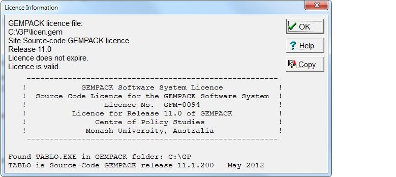
Figure 2.1 GEMPACK licence command
Second, the About/Diagnostics command (also usually under the Help Menu) shows:
- the name and Version no. of the program; eg, ViewHAR Version 3.13
- the location and filename of the EXE file
- if TABLO.EXE is present in your GEMPACK folder, the GEMPACK Version and Release information for that copy of TABLO.EXE
- a Diagnostics button that displays much more information, which can be saved in a file. If you have a problem, GEMPACK support may ask you to send them this "diagnostics file".
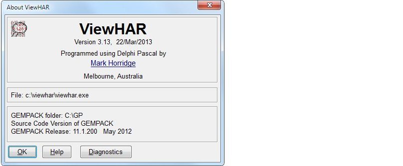
Figure 2.2 About/diagnostics
Program Version and GEMPACK Release Information for Command-line or Fortran-based GEMPACK programs is contained in the first 4 or 5 lines of the log file (if there is one) or in the first 4 or 5 lines of screen output when you run that program from the command-line. Usually this information has scrolled off the top of the Command prompt window before you have time to read it. You may need to scroll back to see it. Or, to capture the output to a file, type:
sltoht <nul: >temp.log
and then examine the top of file temp.log. You might see something like:
 <SLTOHT   Version 5.52  January 2011>
   This program accesses some of the routines in the GEMPACK software release
 <GEMPACK Release 11.1.200   May 2012>
In ViewHAR the History command will show you Program Version and GEMPACK Release Information about the program that created a HAR file — see section 49.1. The same information is echoed to the log whenever a Command-line GEMPACK program reads a HAR file.
3 How to carry out simulations with models [gpd1.2]
Click here for detailed chapter contents
This chapter is where we expect new users of GEMPACK to start learning about simulations. We describe how simulations are carried out, and explain some of the terms used in GEMPACK, such as: implementation, simulation, levels and percentage-change variables.
In section 3.1, there is a very brief overview of the Stylized Johansen model and the simulation that you will carry out. The rest of this chapter consists of detailed instructions for carrying out the simulations and interpreting their results.
We encourage you to work through this whole chapter before starting to work with GEMPACK on your own model. At the end of this chapter we suggest different directions you may wish to go in.
Implementation
A model is implemented in GEMPACK when
- the equations describing its economic behaviour are written down in an algebraic form, following a syntax described later in this document, and
- data describing one solution of the model are assembled, to be used as a starting point for simulations.
For most GEMPACK models, the equations are written down in a linearized form, usually expressed in terms of percentage changes in the variables. But you can choose instead to write down the original (or "levels") equations. In either case you need to write them down in a text file which we call a TABLO Input file or TAB file, since TABLO is the name of the GEMPACK program which processes this information.
The procedure for implementing models is described in detail in chapter 4.
Simulation
Once a model is implemented, the model can be used to carry out simulations. Many simulations are the answer to "What if" questions such as "If the government were to increase tariffs by 10 percent, how much different would the economy be in 5 years time from what it would otherwise have been?". From the original solution supplied as the starting point, a simulation calculates a new solution to the equations of the model. GEMPACK usually reports the results of a simulation as percentage changes from the original solution. Levels results may also be available.
Solving models
within GEMPACK is always done in the context of a simulation. You specify the values of certain of the variables (the exogenous ones) and the software calculates the values of the remaining variables (the endogenous ones).
The new values of the exogenous variables are usually given by specifying the percentage changes (increases or decreases) from their values in the original solution.
Levels and Percentage-Change Variables
When the model is implemented, the equations may be linearized (that is, differentiated). The variables in these linearized equations are usually interpreted as percentage changes in the original variables. The original variables (prices, quantities etc) are referred to as the levels variables and the (usually nonlinear) equations relating these levels variables are called the levels equations.
For example, the levels equation
V = P Q
relates the dollar value V of a commodity to its price P ($ per ton) and its quantity Q (tons). The linearized version of this is
p_V = p_P + p_Q
(as explained later in chapter 4 below) which says that, to first order, the percentage change p_V in the dollar value is equal to the sum of the percentage changes p_P in the price and p_Q in the quantity.
Data
The data for a model often consists of input-output data (giving dollar values) and parameters (including elasticities). The data given are usually sufficient to read off an initial solution to the levels equations. (Usually all basic prices are taken as 1 in the initial solution.)
3.1 An example simulation with stylized Johansen [gpd1.2.1]
In this chapter we show you how to carry out simulations with an existing model (that is, one built by someone else). We use as an example the Stylized Johansen model described in Chapter 3 of Dixon et al (1992), hereafter referred to as DPPW. The model equations are listed in table 4.1 in section 4.1.
The Stylized Johansen model is chosen because it is simple. Once you know how to carry out simulations with it in GEMPACK, you will find it easy to carry out simulations with other, more complicated models (including ones you build yourself).
3.1.1 Introduction to the stylized Johansen model [gpd1.2.1.1]
The Stylized Johansen model is a very simple model of a single country. It recognises two sectors "s1" and "s2" each producing a single commodity, one final demander (households) and two primary factors (labor and capital). There are no exports or imports. Output of each sector is a Cobb-Douglas aggregate of labor, capital, and intermediate inputs. Household demands are also Cobb-Douglas.
The initial input-output data base is shown below in Table 3.1. For example, households consume 4 (million) dollars' worth of commodity 2 and industry 2 uses 3 (million) dollars' worth of labor. Note that the first two row totals (value of sales each of good) equal the first two column totals (costs of each sector).
Table 3.1 Input-output data base for Stylized Johansen
| Demanders: | Industry 1 | Industry 2 | Households | Total Sales | |
| Inputs | |||||
| Commodity | 1 | 4.0 | 2.0 | 2.0 | 8.0 |
| Commodity | 2 | 2.0 | 6.0 | 4.0 | 12.0 |
| Labor | 3 | 1.0 | 3.0 | 4.0 | |
| Capital | 4 | 1.0 | 1.0 | 2.0 | |
| Total Production | 8.0 | 12.0 | 6.0 |
In the GEMPACK implementation, the levels variables are as in Table 3.2 below.
Table 3.2 Levels variables of Stylized Johansen
| GEMPACK variable | Meaning | DPPW | Notation |
| Y | Value of household income | Y | |
| PC(i) | Price of commodity i | Pi | (i=1,2) |
| PF(f) | Price of factor f | Pf | (f=3,4) |
| XCOM(i) | Supply of commodity i | Xi | (i=1,2) |
| XFAC(f) | Supply of factor f | Xf | (f=3,4) |
| XH(i) | Household use of commodity i | Xi0 | (i=1,2) |
| XC(i,j) | Intermediate input of commodity i to industry j | Xij | (i,j=1,2) |
| XF(f,j) | Input of factor f to industry j | Xfj | (f=3,4;j=1,2) |
| DVCOMIN(i,j) | Dollar values for intermediate inputs | (i,j=1,2) | |
| DVFACIN(f,j) | Dollar values for factor use by industry | (f=3,4;j=1,2) | |
| DVHOUS(i) | Dollar values for household consumption | (i=1,2) |
Note that most of the variables have one or more arguments (indicating associated sectors and/or factors). We refer to such variables as vector or matrix variables. For example, PC(i) is a vector variable with 2 components, one for each sector, namely PC("s1") and PC("s2"). XF(f,j) is a matrix variable with the following 4 components:
| component 1 XF("labor","s1") | input of labor (factor 1) to sector 1 |
| component 2 XF("capital","s1") | input of capital (factor 2) to sector 1 |
| component 3 XF("labor","s2") | input of labor (factor 1) to sector 2 |
| component 4 XF("capital","s2") | input of capital (factor 2) to sector 2 |
Variables which have no arguments ('Y' is the only one here) are referred to as scalar or macro variables.
Corresponding to each levels variables, there is an associated percentage change variable. TABLO adds the prefix "p_" to the name of the levels variable to indicate a percentage change. For example, p_XF is the percentage change in the levels variable XF. In DPPW, lower case letters are used to denote percentage-change variables.
More details about the model are given in chapter 4. A full TABLO Input file can be found in section 4.3.3.
3.1.2 The simulation [gpd1.2.1.2]
In the example simulation with the Stylized Johansen model used throughout most of this chapter, we choose a closure in which supplies of the two factors, labor and capital, are the exogenous variables. This means we will specify the percentage changes in the variable XFAC, namely p_XFAC, and solve the model to find the percentage changes in all the other variables. You will also be able to see the levels results (for example, the post-simulation value of household income).
For this simulation, we increase the supply of labor by 10 per cent and hold the supply of capital fixed.
The starting points for any simulation with the Stylized Johansen model are
- the TABLO Input file, SJ.TAB, and
- the data file, SJ.HAR.
3.2 Preparing a directory for model SJ [gpd1.2.4.2]
We assume that you have already installed GEMPACK correctly as described in chapter 2.
To keep all example files for the Stylized Johansen model together in one area, you should first create a separate directory (folder) for these files and copy the relevant files into this directory.
Use Windows Explorer (or My Computer) to create a new folder or subdirectory called \sj and copy all the sj*.* files from the directory containing the GEMPACK model examples (usually C:\GP\EXAMPLES) to this directory \sj.
3.3 Using GEMPACK: WinGEM or command prompt? [gpd1.2.3]
There are two ways of operating GEMPACK:
- through the WinGEM interface. Initially this method is easier, since WinGEM helps you with the names of the programs and files used by GEMPACK.
- at the Command line, ie, working in a DOS box within Windows. We will refer to this method as Command Prompt. Many advanced users find this approach quicker and more flexible. They use DOS commands but also launch Windows programs such as TABmate, ViewHAR and ViewSOL from the command line.
We describe both methods, but suggest that you first work through this chapter using the WinGEM method — then, if you wish, repeat the exercise using the Command prompt instructions which are shown like this:
Command-prompt users should read (but not do) the WinGEM instructions, then should execute the corresponding DOS commands, which will be shown just after the WinGEM instructions.
3.4 Stylized Johansen example simulation [gpd1.2.4]
3.4.1 Starting WinGEM [gpd1.2.4.1]
In Windows, double-click on the WinGEM icon to start GEMPACK for Windows. The main WinGEM menu should appear, as a ribbon menu across the top of the screen:
WinGEM - GEMPACK for Windows
File Simulation HA Files Other tasks Programs Options Window Help
3.4.2 Setting the working directory [gpd1.2.4.3]
WinGEM uses the idea of a working directory to simplify choosing files and running programs. This working directory is where all the files for the model you are using are stored.
For the Stylized Johansen model examples here, the working directory needs to be the directory \SJ you have just created. To set this, first click on File in the main WinGEM menu. This will produce a drop-down menu. In the drop-down menu, click on the menu item Change both default directories.
The notation we use for this sequence of clicks (first File then Change both default directories) is
File | Change both default directories.
In the file selection box that appears, choose drive C: (or the drive containing your directory \SJ if it is on a different drive). Then double-click on C:\ (this will be at the top of the list of directories shown) and then double-click on the subdirectory SJ. [Make sure that the directory name shown in blue above the selection box changes to C:\SJ (or D:\SJ etc if your \SJ directory is on another drive).] Click on the Ok button.
Command-prompt users should open a DOS box in the C:\sj directory.1
3.4.3 Looking at the data directly using ViewHAR [gpd1.2.4.4]
The input-output data used in the Stylized Johansen model are contained in the data file SJ.HAR. This is a special GEMPACK binary file - called a Header Array file - so you cannot just look at it in a text editor. Instead you will look at SJ.HAR using the ViewHAR program. Select from the main WinGEM menu: HA Files | View VIEWHAR
The ViewHAR window will appear. Click on File | Open and select the file SJ.HAR. This will open the file SJ.HAR and show its contents on the Contents screen.
Command-prompt users can open SJ.HAR by typing "viewhar SJ.HAR" into the DOS box.
Each row of the ViewHAR Contents screen corresponds to a different array of data on the file. Look at the "Name" column to see what data are in these arrays.
| Header | Type | Size | Name | |
| 1 | CINP | RE | SECTxSECT | Intermediate inputs of commodities to ind. |
| 2 | FINP | RE | SECTxFACT | Intermediate inputs of primary factors - dollar |
| 3 | HCON | RE | SECT | Household use of commodities - dollar values |
The first array is the "Intermediate inputs of commodities to industries - dollar values". The Header CINP is just a label for this array (headers can have up to 4 characters). The array is of Type RE — an array of real numbers with set and element labelling (see chapter 5.0.3).
Double-click on CINP to see the numbers in this array.
| DVCOMIN | s1 | s2 | Total | |
| s1 | 4.00 | 2.00 | 6.00 | |
| s2 | 2.00 | 6.00 | 8.00 | |
| Total | 6.00 | 8.00 | 14.00 |
Compare these numbers with the input-output data for Stylized Johansen shown in Table 3.1. The actual data in the file at this header is just the 2x2 matrix. ViewHAR calculates and shows the row and column totals.
To return to the Contents Screen, click on Contents in the ViewHAR menu, or click twice on any number.
Look at the other Header Arrays called FINP and HCON to see where their numbers fit in the input-output data base.
Close ViewHAR by selecting File | Exit.
3.5 Implementing and running model SJ [gpd1.impsj]
There are three steps involved in carrying out a simulation using GEMPACK.
Step 1 - Implement the model (using TABLO)
Step 2 - Solve the equations of the model (ie, run a simulation)
Step 3 - View the results
3.5.1 TABLO-generated program or GEMSIM? [gpd1.2.4.5]
The details of steps 1 and 2 vary according to whether you have the Executable-image or the Source-code version of GEMPACK. With either version, you can use GEMSIM to run simulations. The Source-code version also allows you to create a model-specific, TABLO-generated, EXE file, which you can run to solve the model. Especially for larger models, the TABLO-generated program will usually solve quicker.
The Source-code method is described next. If you have the Executable-image version of GEMPACK, you will need to skip onto the GEMSIM instructions in section 3.5.3.
3.5.2 Source-code method: using a TABLO-generated program [gpd1.2.4.6]
In the next examples we are assuming that you have the Source-code version of GEMPACK and have a Fortran compiler on your DOS PATH.
From the WinGEM menu at the top of the screen choose Simulation. In the drop-down menu the choices are
TABLO Implement
Compile & Link
TABmate Implement
-------------------
Run TG Program
GEMSIM Solve
SAGEM Johansen Solve
---------------------
View Solution (ViewSOL)
AnalyseGE
The items from this menu you will be using in this simulation are
TABLO Implement
Compile & Link
Run TG Program
View Solution (ViewSOL).
In the TABLO-generated program method, the GEMPACK program TABLO is used to convert the algebraic equations of the economic model into a Fortran program (.FOR file) specific to your model. This Fortran program (which is referred to as the TABLO-generated program or TG Program in the above menu) is compiled and linked to a library of GEMPACK subroutines. The EXE file of the TABLO-generated program produced by the compiler is used to run simulations (instead of using the program GEMSIM). This method provides faster execution times for large models than the GEMSIM alternative but means you must have an appropriate Fortran compiler.
WinGEM will guide you through the various steps and indicate what to do next.
Step 1 - Implementing the model SJ using TABLO
Step 1(a) - Run TABLO to create the TABLO-generated program
The TABLO Input file is called SJ.TAB. It contains the theory of the Stylized Johansen model. Choose
Simulation | TABLO Implement
A window for TABLO will appear. Click on the Select button to select the name of the TABLO Input file SJ.TAB2. This is all TABLO needs to implement this model. 3
At top right of the TABLO window are choice buttons for FORTRAN and GEMSIM.
Check that the first, FORTRAN, option is selected (we want you to create the TABLO-generated Fortran program).
Click on the Run button. The program runs TABLO in a DOS box and when complete, returns you to the TABLO window with the names of files it has created: the Information file SJ.INF and the Log file. Look at both of these files by clicking the View buttons beside them.
The Information file SJ.INF gives information about the TABLO Input file such as whether there are any syntax or semantic errors during checking by TABLO. Search the file for %% to see if there are any errors. Search the file for "syntax error" to see how many syntax errors and semantic problems there are (hopefully none). Go to the end of the file to see what actions can be carried out by the TABLO-generated program produced in this TABLO run.
Command-prompt users can perform Step 1(a) by typing "tablo -wfp sj -log sj.log". To see LOG or INF files, type "tabmate SJ.INF" or "tabmate SJ.LOG".
Step 1(b) - Compile and Link the TABLO-generated Program
When you have looked at these two files, click on the Go to Compile and Link button at the bottom of the TABLO window to run the Fortran compiler. (Alternatively you can start this window by choosing Simulation | Compile and Link... from WinGEM's main menu.)
In the Compile and Link window, the file SJ.FOR is already selected as the TG Program Name. Click on the button Compile and Link and wait a little while the compiler converts the Fortran file SJ.FOR into the SJ.EXE program that you can run.
When finished, click on the button Go to 'Run TG Program' to proceed to the next step in running a simulation.
Command-prompt users can perform Step 1(b) by typing "LTG sj". Type "dir sj.exe" to check that file SJ.EXE has been produced.
Step 2 - Solve the equations of the model using TABLO-generated program
The Go to 'Run TG Program' button takes you to the window for running the TABLO-generated program SJ.EXE. (Alternatively you can start this window by choosing Simulation | Run TG Program... from WinGEM's main menu.)
First Select the Command file called SJLB.CMF. Since Command files are text files, look at this Command file in the text editor by clicking the Edit button.
How is the closure specified? What shock is applied?
What data file is used by this model? How many steps are used in the multi-step solution?
Details about using a GEMPACK Command file to specify a simulation are given in section 3.8 below. For the present, we suggest that you take this on trust and continue with the simulation.
Select File | Exit to close the editor and return to the "Run TG Program" window.
Click on Run to run SJ.EXE with the Command file SJLB.CMF.
When SJ.EXE finishes running, an accuracy summary window will pop up. This gives a graphical view as to how accurately the equations have been solved4. You can ignore this for the present (it is discussed in section 3.12.3) so click OK.
If SJ.EXE produces the Solution file, click on Go to ViewSOL5.
If there is an error, view the Log file.
Command-prompt users can examine the Command file SJLB.CMF by typing "TABmate SJLB.CMF". Run the simulation by typing "sj -cmf SJLB.CMF". Then, to see the results, type "ViewSOL SJLB.SL4".
Now please skip the next (GEMSIM) section and go on to the ViewSOL instructions in 3.5.4.
3.5.3 Executable-image method: using GEMSIM [gpd1.2.4.7]
In the WinGEM menu at the top of the screen choose Simulation. In the drop-down menu the choices are6.
TABLO Implement
Compile & Link
TABmate Implement
-------------------
Run TG Program
GEMSIM Solve
SAGEM Johansen Solve
---------------------
View Solution (ViewSOL)
AnalyseGE
The items from this menu you will be using in this simulation are
TABLO Implement
GEMSIM Solve
View Solution (ViewSOL).
WinGEM will guide you through the various steps and indicate what to do next.
Step 1 - Implementing the model SJ using TABLO (for GEMSIM output)
The TABLO Input file is called SJ.TAB. It contains the theory of the Stylized Johansen model. Choose Simulation | TABLO Implement...
A window for TABLO will appear. Click on the Select button to select the name of the TABLO Input file SJ.TAB7. This is all TABLO needs to implement this model 8.
At top right of the TABLO window are choice buttons for FORTRAN and GEMSIM.
Check that the second, GEMSIM, option is selected (we want you to create the GEMSIM Auxiliary files).
By "implement" we mean convert the TABLO Input file into binary computer files which are used by the simulation program GEMSIM in the next step. These files are referred to as Auxiliary files (or sometimes as the GEMSIM Statement and Table files) and in this case, are called SJ.GSS and SJ.GST.
Click on the Run button. The program TABLO runs in a DOS box and when complete returns you to the TABLO window with the names of files it has created: the Information file SJ.INF and the Log file. Look at both of these files by clicking the View buttons beside them. To close the file, click on the X in the top right-hand corner of the view, or click File..Exit using the File menu.
The Information file SJ.INF gives information about the TABLO Input file such as whether there are any syntax or semantic errors found during checking by TABLO. Search the file for %% to see if there are any errors. Search the file for "syntax error" to see how many syntax errors and semantic problems there are (hopefully none). Go to the end of the file to see what actions GEMSIM can carry out with the Auxiliary files produced in this TABLO run.
When you have looked at these two files, click on the Go to GEMSIM button at the bottom of the TABLO window to go on to the next step in running a simulation:
Command-prompt users can perform Step 1 by typing "tablo -pgs sj -log sj.log". To see LOG or INF files, type "tabmate SJ.INF" or "tabmate SJ.LOG".
Step 2 - Solve the equations of the model using GEMSIM
The Go To GEMSIM button takes you to the GEMSIM window. (Alternatively you can start this window by choosing Simulation | GEMSIM Solve from WinGEM's main menu.)
First Select the Command file called SJLB.CMF. Since Command files are text files, look at this Command file in the text editor by clicking the Edit button.
How is the closure specified? What shock is applied?
What data file is used by this model? How many steps are used in the multi-step solution?
Details about using a GEMPACK Command file to specify a simulation are given in section 3.8 below. For the present, we suggest that you take this on trust and continue with the simulation.
Select File | Exit to close the editor and return to the GEMSIM window.
Click on Run to run GEMSIM with the Command file SJLB.CMF.
When GEMSIM finishes running, an accuracy summary window will pop up. This gives a graphical view as to how accurately the equations have been solved9. You can ignore this for the present (it is discussed in section 3.12.3) so click OK.
If GEMSIM produces the Solution file, click on Go to ViewSOL10.
If there is an error, view the Log file.
Command-prompt users can examine the Command file SJLB.CMF by typing "TABmate SJLB.CMF". Run the simulation by typing "sj -cmf SJLB.CMF". Then, to see the results, type "ViewSOL SJLB.SL4".
3.5.4 Step 3 - View the Solution using ViewSOL [gpd1.2.viewsol]
You cannot view the Solution file SJLB.SL4 in a text editor because it is a binary file, not a text file. Instead we use ViewSOL to examine the Solution file.
In WinGEM, the Go to ViewSOL button starts the program ViewSOL running and opens the Solution file SJLB.SL4 . [Alternatively you can start this window by choosing Simulation | View Solution (ViewSOL) from WinGEM's main menu.]
Command-prompt users should type "ViewSOL SJLB.SL4".
You will see the Contents page listing many of the variables of the model. ViewSOL has 3 slightly different formats for this Contents list. Select Format... from ViewSOL's main menu and there click on Arrange vectors by name (in the panel headed Vector options); then click Ok which will put you back to the Contents list.
To see the results of one of these variables listed by name, just double-click on the corresponding row in the Contents list. First double-click on the p_XCOM row to see the results for this variable (demand for the two commodities). Select 3 decimal places (see the third drop-down list box along the top row of the current ViewSOL window - the only one with a single figure in it). Then you should see something like the following:
| p_XCOM | sjlb | Pre sjlb | Post sjlb | Ch/%Ch sjlb |
| s1 | 5.885 | 8.000 | 8.471 | 0.471 |
| s2 | 6.899 | 12.000 | 12.828 | 0.828 |
Across the s1 row you see the percentage change result (5.885%), the pre-simulation levels value (8.000), the post-simulation levels value (8.471) and the change (0.471); these are the results for the total supply of commodity s1.
Then click on Contents to return to the Contents list.
To see the p_XFAC results, double-click on this row. You will see
| p_XFAC | sjlb | Pre sjlb | Post sjlb | Ch/%Ch sjlb |
| labor | 10.000 | 4.000 | 4.400 | 0.400 |
| capital | 0 | 2.000 | 2.000 | 0 |
This time all the numbers are in red which is used to remind you that, for this simulation, both components of this variable p_XFAC are exogenous. You should easily be able to understand all of these results.
Then click on Contents to return to the Contents list (or click twice on any number).
To see the p_XC(i,j) results [intermediate inputs of commodity i into industry j], double-click on this row. Now you see
| p_XC | s1 | s2 |
| s1 | 5.885 | 5.885 |
| s2 | 6.899 | 6.899 |
and, in the second drop-down box you should see "1 sjlb". This indicates that you are just seeing the linearized simulation results (the percentage changes in the four components of this variable). You can't see the pre- and post-simulation levels results at the same time since this variable p_XC is a matrix variable. To see the pre-simulation levels results, click on the second drop-down list box (the one showing "1 sjlb") and select the second alternative ("2 Pre sjlb"). Then you will see the pre-simulation levels results. You might also like to look at the post-simulation levels results and the changes.
Then click on Contents to return to the Contents list.
When you have finished looking at the results, exit from ViewSOL.
3.6 The steps in carrying out a simulation [gpd1.2.5]
This section recapitulates the steps (that you just followed) to implement a model and carry out a simulation.
In all cases, after the TABLO Input file for a model has been written, there are 3 steps on the computer to carry out a first simulation with the model. These steps are:
Step 1 - Implement the model
Step 2 - Simulation (Solve the equations of the model)
Step 3 - View the results with ViewSOL or perhaps AnalyseGE.
Step 1 always involves running the program TABLO.
The details of Steps 1 and 2 are a little different depending on whether you have a Source-code or Executable-image version of GEMPACK, as we explain below.
Next we describe the Source-code procedure. The Executable-image version of steps 1 and 2 is described in section 3.6.2.
3.6.1 Steps 1 and 2 using a TABLO-generated program (source-code GEMPACK) [gpd1.2.5.1]
The steps are illustrated in Figure 3.1 below.
Figure 3.1 The steps in carrying out a simulation using a TABLO-generated program
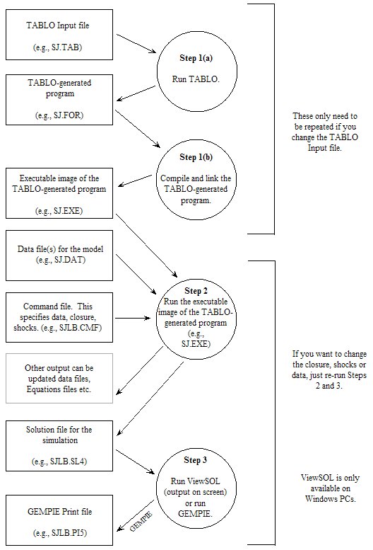
Step 1. Computer Implementation of the Model
Step 1(a) - Run TABLO to create TABLO-generated program
Process the TABLO Input file for the model by running the program TABLO. Select the option WFP which tells TABLO to write a Fortran program (referred to as the TABLO-generated program of the model) which captures the theory of the model.
Step 1(b) - Compile and Link the TABLO-generated program [LTG]
Compile and link the TABLO-generated program of the model, produced in Step 1(a). This will produce an EXE file of the TABLO-generated program11.
Step 2. Simulation (Solve the equations of the model)
Run the EXE file of the TABLO-generated program, as produced in Step 1(b). Take inputs from a Command file which tells the program which base data files are to be read and describes the closure (that is, which variables are exogenous and which are endogenous) and the shocks. This program then computes the solution to your simulation and writes the results to a Solution file
Step 3. Printing or Viewing the Results of the Simulation
The last step is to view simulation results with ViewSOL or AnalyseGE12. An alternative is to use the program SLTOHT to process results (for example, to produce tables for reports), as introduced in section 3.10 below.
3.6.2 Steps 1 and 2 using GEMSIM [gpd1.2.5.2]
The steps using GEMSIM are illustrated in Figure 3.2.
Figure 3.2 The steps in carrying out a simulation using GEMSIM
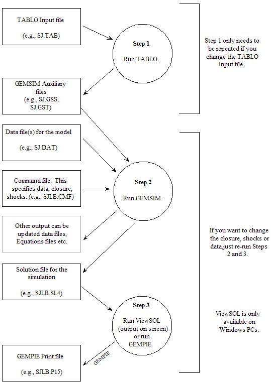
Step 1. Computer Implementation of the Model
Process the TABLO Input file for the model by running the GEMPACK program TABLO. Select the option PGS which asks TABLO to produce the GEMSIM Auxiliary files for the GEMPACK program GEMSIM (see Step 2). These files capture the theory of the model, as written in the TABLO Input file.
Selecting option PGS rather than the option WFP as in section 3.6.1 above is what initiates the GEMSIM route rather than the TABLO-generated program route.
Step 2. Simulation (Solve the equations of the model)
Run the GEMPACK program GEMSIM13 and tell it to use the GEMSIM Auxiliary (GSS/GST) files produced in Step 1. Take inputs from a Command file which tells the program which base data files are to be read and describes the closure (that is, which variables are exogenous and which are endogenous) and the shocks. GEMSIM then computes the solution to your simulation and writes the results to a Solution file.
Step 3. Printing or Viewing the Results of the Simulation
The last step is to view simulation results with ViewSOL or AnalyseGE14. An alternative is to use the program SLTOHT to process results (for example, to produce tables for reports), as introduced in section 3.10 below.
Comparing the steps in the two cases
Note that Step 1 above is very similar to Step 1(a) in the TABLO-generated program case (see section 3.6.1 above). The LTG step 1(b) in section 3.6.1 has no analogue in the GEMSIM case since GEMSIM is a general-purpose program which can be used to solve any model. Step 2 is different only in that GEMSIM is run rather than the TABLO-generated program. Step 3 is identical in the two cases.
3.6.3 Other Simulations [gpd1.2.5.othsims]
Once you have carried out one simulation with a model, you will probably want to carry out others, for example, to change the closure and/or shocks, or even to run from different base data. In such cases, you do not have to repeat Steps 1(a) and 1(b). All you have to do is carry out Steps 2 and 3. A hands-on example is given in section 3.11 below. (Of course Step 1 must be repeated if you change the TABLO Input file in any way.)
3.7 Interpreting the results [gpd1.2.7]
You have already looked at the results via ViewSOL (see Step 3 in section 3.5.4). From the ViewSOL Contents page you clicked on and examined variables such as Macros, p_XH, p_PC, p_XF, p_DVHOUS. We have copied some of the results from ViewSOL to a spreadsheet (via the Copy menu item in ViewSOL). These are shown in Table 3.3 below.
We think that you will find the tables fairly easy to interpret.
Table 3.3 Results (ViewSOL) from the solution file SJLB.SL4
| Macros | sjlb | Pre sjlb | Post sjlb | Chng sjlb |
| p_Y | 5.8853 | 6.0000 | 6.3531 | 0.3531 |
| p_XH | sjlb | Pre sjlb | Post sjlb | Chng sjlb |
| s1 | 5.8853 | 2.0000 | 2.1177 | 0.1177 |
| s2 | 6.8993 | 4.0000 | 4.2760 | 0.2760 |
| p_PC | sjlb | Pre sjlb | Post sjlb | Chng sjlb |
| s1 | 0.0000 | 1.0000 | 1.0000 | 0.0000 |
| s2 | -0.9486 | 1.0000 | 0.9905 | -0.0095 |
| p_XF | s1 | s2 | ||
| labor | 10.0000 | 10.0000 | ||
| capital | 0.0000 | 0.0000 | ||
| p_DVHOUS | sjlb | Pre sjlb | Post sjlb | Chng sjlb |
| s1 | 5.8853 | 2.0000 | 2.1177 | 0.1177 |
| s2 | 5.8853 | 4.0000 | 4.2354 | 0.2354 |
The results show what happens if the supply of labor is increased by 10 per cent and the supply of capital is held fixed. For example,
- Look at the simulation result for 'p_Y', the percentage change in the levels variable 'Y'. The dollar value of total nominal household expenditure will increase by 5.8853 per cent from its pre-simulation value of 6.0000 to its post-simulation value of 6.3531.
- Look at the results for p_XH. The result for commodity 2, p_XH ("s2"), shows that households will consume 6.8993 per cent more of commodity 2 than they did previously.
- Look at the results for p_PC. The price of commodity 2 will fall by 0.9486 per cent.
- The simulation results for p_DVHOUS show that the dollar value of household consumption of commodity 2 will rise by 5.8853 per cent from its pre-simulation value of 4.0000 to its post-simulation value of 4.2354.
Recall that, within GEMPACK, all simulations are set up and solved as perturbations from an initial solution, and results are usually reported as changes or percentage changes from this original solution. In this case the original solution values are as shown in Table 3.2 above, which shows million dollar values of activity. Suitable levels values for quantities can be obtained by assuming that, initially, all prices are 1. (This just sets the units in which quantities are measured.) Then, for example, since households consume 4 million dollars' worth of commodity 2, this means that they consume 4 million units of that commodity.
Hence the three simulation results mentioned above mean that, once labor is increased by 10 per cent and capital is held fixed:
1. Total nominal household expenditure Y has increased to approximately 6.353 million dollars (5.8853 per cent more than the original value of 6 million dollars).
(The other three values given with p_Y in Table 3.3 are
| 6.0000 | which is the pre-simulation level of Y, |
| 6.3531 | which is the post-simulation level of Y and |
| 0.3531 | the change between these two values.) |
2. Household consumption (XH) of commodity 2 has increased to 4.2760 million units (6.8993 per cent more than the original 4 million units).
3. The commodity price (PC) of commodity 2 has fallen from one dollar per unit to approximately 99.051 cents per unit (a fall of 0.9486 per cent).
4. The dollar value of household consumption (DVHOUS) of the commodity produced by sector "s2" has risen from 4 million dollars to approximately 4.2354 million dollars (an increase of 5.8853 per cent).
The updated values in (2), (3) and (4) above should be related since dollar value should equal price times quantity. The levels equation for commodity 2 ("s2") is
DVHOUS("s2") = PC("s2) x XH("s2")
Note that this equation is true for the post-simulation values, since, from (2) and (3) above, the post-simulation price times the post-simulation quantity is
| 0.99051 x 4.2760 = 4.2354 |
which is equal to the post-simulation dollar value in (4). This confirms that the solution shown in ViewSOL satisfies the levels equation connecting price, quantity and dollar value of household consumption of this commodity. You might like to check some of the other levels equations in this way.
3.8 Specifying a simulation [gpd1.2.8]
In order to specify the details for carrying out a simulation, you must
- say which model to use,
- say which base data to begin from (that is, the pre-simulation solution),
- say which closure (that is, which variables are endogenous and which are exogenous), and
- say which variables to shock, and by how much, and
- specify the names of the various output files.
Figure 3.3 The information required to specify a simulation
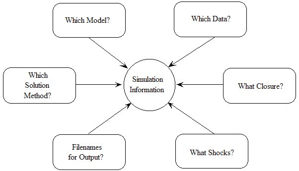
Within GEMPACK, the normal way of specifying this information to the software is via a Command (CMF) file. Indeed, when you carried out the example simulation above, this is exactly what happened in Step 2 above since there you ran either the TABLO-generated program or GEMSIM and took inputs from the Command file SJLB.CMF.
The instructions in this Command file must be prepared in advance in a text editor.
The next section explains the statements in this GEMPACK Command file SJLB.CMF.
3.8.1 Specifying a simulation via a GEMPACK command file [gpd1.2.8.1]
In Step 2 of the example simulation, the program took all the information required to specify the simulation from the GEMPACK Command file SJLB.CMF. The file SJLB.CMF is shown in full in Figure 3.4 below.
Figure 3.4 The GEMPACK command file SJLB.CMF
! The following GEMPACK Command file (usually called SJLB.CMF)
!  carries out a multi-step simulation
!  for the Stylized Johansen model.
!  Auxiliary files (usually tells which TAB file)
auxiliary files = sj ;
! Data files
file iodata = SJ.HAR ;
updated file iodata = <cmf>.upd ;
! Closure
exogenous p_xfac ;
rest endogenous ;
! Solution method information
method = euler ;
steps = 1 2 4 ;
! Simulation part
! Name of Solution file is inferred from name of Command file
! (See section 20.5.)
shock  p_xfac("labor") = 10 ;
verbal description =
Stylized Johansen model. Standard data and closure.
10 per cent increase in amount of labor. (Capital remains unchanged.) ;
! Options.extrapolation accuracy file = yes ;
log file = yes ;
! End of Command file
The statements in SJLB.CMF are discussed briefly below.
The statement
auxiliary files = sj ;
tells GEMSIM or the TABLO-generated program to use the Auxiliary files produced in Step 1. (This effectively tells which TABLO Input file (or model) to work with, since these files are just a processed version of the TABLO Input file SJ.TAB for the Stylized Johansen model.) [If you are using the TABLO-generated program SJ.EXE, the Auxiliary files are SJ.AXS and SJ.AXT produced when you ran TABLO in Step 1. If you are using GEMSIM, the Auxiliary files are SJ.GSS and SJ.GST produced when you ran TABLO in Step 1.]. You can find more details about these Auxiliary files in 21.
The statement
file iodata = SJ.HAR ;
tells SJ.EXE or GEMSIM to read base data from the file SJ.HAR (which contains the data in Table 3.1 above).
The line
! Data files
above this line is a comment since it begins with an exclamation mark !. While such comments are ignored by the software, they are very important in organising and documenting the Command file and in making it an intelligible record of the simulation. [You can see several other comment lines in the file.]
The statements:
exogenous p_xfac ;
rest endogenous ;
give the closure (that is, which variables to take as exogenous and which to take as endogenous), while the statement
shock p_xfac("labor") = 10 ;
gives the shock needed to increase the supply of labor by 10 per cent.
When the TABLO-generated program SJ or GEMSIM carries out a simulation, as well as being able to report the changes in the endogenous variables, the program produces an updated version of the original data file(s). The data in these updated data files represent post-simulation values (that is, the ones that would hold after the shocks have worked their way through the economy). For Stylized Johansen, this contains post-simulation dollar values of the entries in Table 3.1 above. The statement
updated file iodata = <cmf>.upd ;
names the file to contain this updated data [examined in section 3.9 below]. The <cmf> in this line indicates that this part of the name comes from the name of the Command file. Since the Command file is usually called SJLB.CMF, the program replaces <cmf> by SJLB (the name of the Command file ignoring its suffix .CMF) so that the updated iodata file will be called SJLB.UPD. The <cmf> syntax is explained further in section 20.5.
The most important output from a simulation is the Solution file which contains the results for the percentage changes in prices and quantities. Here we have omitted the name of the Solution file so the name of this file is taken from the name of the Command file. Because the Command file is called SJLB.CMF, the Solution file will be called SJLB.SL4 (the same basic name SJLB followed by .SL4 which is the standard GEMPACK suffix for Solution files). Another alternative is to add a statement of the form
solution file = ... ; ! Not included in this SJLB.CMF
in the Command file. Such a statement is allowed, but it is customary to omit it so that the name of the Solution file is inferred from the name of the Command file.
You are required to give a verbal description of the simulation. This description, which can be several lines of text, goes on the Solution file and is visible from ViewSOL and other programs. You can use this to remind yourself (and others) about salient features of the simulation. The statement
verbal description = .Stylized Johansen model.
 Standard data and closure.
 10 per cent increase in amount of labor (Capital remains unchanged.)
 1,2,4-step solutions plus extrapolation. ;
in SJLB.CMF give 4 lines of text for the verbal description in this case. The semicolon ';' indicates the end of this description — indeed all statements in GEMPACK Command files must end with a semicolon ';'.
With GEMPACK, you can choose one of 4 related solution methods for each simulation. These are introduced in section 3.12.3 below. The statements
method = euler ;
steps = 1 2 4 ;
in the Command file tell the program to use Euler's method based on 3 separate solutions using 1, 2 and 4 steps respectively. (See section 3.12.3 below for an explanation about step numbers.)
The accuracy of the solution depends on the solution method and the numbers of steps. SJ.EXE or GEMSIM can be asked to provide information about the accuracy on an Extrapolation Accuracy file. The statement
extrapolation accuracy file = yes ;
asks the program to produce such a file. The information on this file is described in section 3.12.3 below. (The name of this file is the same as that of the Solution file except that it has a different suffix, namely '.XAC', which makes the full name SJLB.XAC.)
The statement
log file = yes ;
asks the software to produce a LOG file showing all the screen activity as the program runs. This LOG file is called SJLB.LOG - it takes its name from the name SJLB.CMF of the Command file but changes the suffix from .CMF to .LOG. This LOG file is a useful record of the simulation.
Further details of Command files and running simulations are given in chapters 19 and following, which describe running simulations with GEMSIM, TABLO-generated Programs and SAGEM. A summary of the statements that can be used in a GEMPACK Command file for running TABLO-generated programs or GEMSIM is given in chapter 35.
In particular, we know that new users of GEMPACK find the auxiliary files (the statement above is "auxiliary files = sj ;") and the file statements (the statements above are "file iodata = SJ.HAR; " and "updated file iodata = <cmf>.upd ;") confusing initially. More details about these can be found in chapters 21 and 22.
3.9 The updated data - another result of the simulation [gpd1.2.9]
Once the simulation shocks have worked their way through the economy, prices and quantities change (as reported by the simulation results). These price and quantity changes imply changes in the values contained in the original data base for the model. When you carry out a simulation, the GEMPACK programs compute these new values. These new values are written to a file which is referred to as the updated data or post-simulation data.
As you saw in section 3.8 above, the line
updated file iodata = <cmf>.upd ;
in the Command file SJLB.CMF means that, when you ran the simulation, the software produced the updated data file SJLB.UPD. This file contains the data as it would be after the shocks (in this case, the increase in labor supply) have worked their way through the model.
You learned in section 3.4.3 how to use ViewHAR to look at the base (or pre-simulation) data file SJ.HAR. This file is the starting point for the simulation; and, when you look at this file you see the numbers shown in Table 3.1 above.
You can also use ViewHAR to look at the updated data in file SJLB.UPD.
If you are using WinGEM, select from the main WinGEM menu : HA Files | View VIEWHAR. The ViewHAR window will appear. Click on File | Open... and select the file SJLB.UPD.
Command-prompt users can open SJLB.UPD by typing "viewhar SJLB.UPD" into the DOS box.
In ViewHAR's contents screen, each row corresponds to a different array of data on the file. Look at the column under the heading "Name" to see what data are in these arrays. Look at values within the three arrays.
You can check that these post-simulation values are consistent with the results of the simulation as discussed in section 3.7 above. For example, the p_DVHOUS results in Table 3.3 show that the value of household expenditure on commodity s2 increased by 5.8853 percent from its pre-simulation value of 4 to its post-simulation value of 4.2354 (which agrees with the Commodity 2 Households value in the table above).
The most obvious results of a simulation are the percentage changes in the variables. The updated data (which is always obtained when you run a simulation) is another important "result" of the simulation, one which is sometimes overlooked. You can look at this updated data to see how the data base has changed as a result of the simulation.
3.10 Preparing tables and graphs for a report [gpd1.2.10]
When you have run some simulations and analysed the simulation results, the next step is usually to write a report containing a selection of the results in tables or graphs.
This section describes how you can transfer simulation results into a spreadsheet program, such as Microsoft Excel. You can use the spreadsheet program to produce tables and graphs which can be copied and pasted into your report.
All the examples below start with the Solution file for Stylized Johansen SJLB.SL4 created in the example simulation described above.
- Example 1 illustrates how to copy directly from ViewSOL into the spreadsheet program.
- Examples 2 and 3 use the command-line program SLTOHT which is documented in sections 39 and 40.
Once you have suitable tables in your spreadsheet program, you can use it to create graphs of the results.
3.10.1 Example 1: Copying from ViewSOL to Spreadsheet and WordProcessor [gpd1.2.viewsolexport]
Open file SJLB.SL4 in ViewSOL. Select Format and then select Arrange vectors by size and set.
In Contents screen, click on the line Vectors size: 2 SECT 4
The Data Window shows the results for all vector variables which range over the set SECT. Use the Decimal Places list box (in middle of upper toolbar) to display at least 4 decimal places.
In the ViewSOL menu, select Export | Copy. This copies the table of numbers to the clipboard.
Open your spreadsheet program and paste into a new spreadsheet. Use the spreadsheet editing to make the table ready for the report. Copy the table from your spreadsheet and paste it into the report document in your word processor, in the usual Windows way. You should see a table like the following.
| p_DVHOUS | p_PC | p_XCOM | p_XH | |
| s1 | 5.8853 | 0 | 5.8853 | 5.8853 |
| s2 | 5.8853 | -0.9486 | 6.8993 | 6.8993 |
ViewSOL has many different Formats that you can use to set up the data to export. Consult the ViewSOL Help for details.
3.10.2 Example 2: Using the GEMPACK Program SLTOHT and Option SSS [gpd1.2.sltoht1]
In the previous example, you interactively pasted from ViewSOL into a spreadsheet the results for one variable.
The SLTOHT method, described here, is more fiddly to set up. However, once you have created a Spreadsheet Mapping file (see below) you can, in one operation, import results for many variables into a spreadsheet. This means that you can automate the production of quite complex reports.
SLTOHT produces a CSV (Comma Separated Value) file. This is a text file which can be opened in your spreadsheet program to import the numbers generated by the simulation. Many arrays, even big arrays with many rows and columns, can be imported, and then (perhaps after some reformatting) moved to your report.
In your text editor, create the file sj1.map which contains just the two lines:
p_xcom
p_xf
This is an example of a Spreadsheet Mapping file (see sections 39.3 and 40.1) used by the program SLTOHT to pick out particular variables on the Solution file.
If you are working in WinGEM, select from the main WinGEM menu
Click on the Select button and choose the Solution file SJLB.SL4.
Choose to print Totals solutions. Click the Ok button.
In the SLTOHT window, select from the menu Options | SLTOHT Options. A screen of SLTOHT option choices will appear. Click on SSS Short SpreadSheet output and select a Comma as separator. (A comma is the default choice.)
Click on Ok to accept these options and return to the main SLTOHT screen.
In the SLTOHT window, select from the menu Options | Use mapping file and select the file SJ1.MAP.
Run the program SLTOHT. This will create the CSV text file called SJLB.CSV. When the program has completed, View the text file SJLB.CSV, which is shown below (after the Command prompt case).
Command prompt Users can start SLTOHT running by typing "sltoht" and entering the responses:
SSS      ! Option SSS
,        ! Data separator is a comma
-SHL     ! Do not include levels results
<carriage-return>    ! Finish option selection
sjlb     ! Name of Solution file
c        ! Cumulative totals
y        ! Yes, use an existing Spreadsheet mapping file
sj1.map  ! Spreadsheet mapping file name
sjlb.csv  ! Name of Output file (CSV)
Look at the file sjlb.csv in your text editor.
The output in file sjlb.csv should look like the box below with the labels and numbers separated by commas. Only the values for variables p_XCOM and p_XF are shown because these were the only two variables in the Spreadsheet Mapping file.
CSV file SJLB.CSV
Solution,sjlb,
 p_XCOM(s1),  5.8852696    ,
 p_XCOM(s2),  6.8992925    ,
 p_XF(labor:s1),  9.9999990    ,
 p_XF(capital:s1),-4.48017488E-07,
 p_XF(labor:s2),  10.000002    ,
 p_XF(capital:s2), 4.48017488E-07,
Start your spreadsheet program (for example Excel) and open the file SJLB.CSV (as a text file with commas for separators). If you format the number cells to show three decimal places, you get a neat spreadsheet table with the labels in one column and the values in the second column. (In a report you would probably want to replace the column of labels with more meaningful labels.)
Document table
| Solution | sjlb |
| p_XCOM(s1) | 5.885 |
| p_XCOM(s2) | 6.899 |
| p_XF(labor:s1) | 10.000 |
| p_XF(capital:s1) | 0.000 |
| p_XF(labor:s2) | 10.000 |
| p_XF(capital:s2) | 0.000 |
3.10.3 Example 3: Using the Program SLTOHT and Option SES [gpd1.2.sltoht2]
There are various different options available in SLTOHT used to produce different kinds of tables as described in chapter 40. Option SES (Spread Sheet with Element labels) produces a table of results using the element names as row and column labels.
In your text editor, create the file sj2.map which contains just the two lines:
p_xcom : p_pc
p_xc
If you are using WinGEM, in the SLTOHT window, select from the WinGEM menu Options | SLTOHT Options. A screen of SLTOHT option choices will appear. Click on SES and select a Comma as separator. (A comma is the default choice.)
Click on Ok to accept these options and return to the main SLTOHT screen.
In the SLTOHT window, select from the menu Options | Use mapping file and select the file SJ2.MAP. Run the program SLTOHT.
SLTOHT will tell you that, by default, this will produce output file SJLB.CSV which already exists. [You created it in Example 2 above.] Click on Yes to say that you wish to change the name of the output file, and choose the name SJLB2.CSV.
When the program has completed, View the text file SJLB2.CSV, which is shown below (after the Command prompt case).
Command prompt Users can start SLTOHT running by typing "sltoht" and entering the responses:
SES      ! Option SES
,        ! Data separator is a comma
-SHL     ! Do not include levels results
<carriage-return>    ! Finish option selection
sjlb     ! Name of Solution file
c        ! Cumulative totals
y        ! Yes, use an existing Spreadsheet mapping file
sj2.map  ! Spreadsheet mapping filename
sjlb2.csv  ! Name of Output file (CSV)
Open the file sjlb2.csv in your spreadsheet program. The values for variables p_XCOM and p_PC are shown side by side and then the array p_XC is shown below, all with element labels.
! Table of 2 variables.
| p_XCOM | p_PC | |
| s1 | 5.885 | 0.000 |
| s2 | 6.899 | -0.949 |
! Variable p_XC # Intermediate inputs of commodity i to industry j #
! Variable p_XC(SECT:SECT) of size 2x2
| s1 | s2 | |
| s1 | 5.885 | 5.885 |
| s2 | 6.899 | 6.899 |
You can import either of these tables into your word processor.
3.10.4 Graphs [gpd1.2.10.1]
Once you have suitable tables in your spreadsheet program, you can use it to create graphs of the results. Alternatively the Charter program supplied with GEMPACK (see section 36.2.1) can be used to produce simple graphs directly from ViewHAR or ViewSOL.
3.11 Changing the closure and shocks [gpd1.2.11]
You can carry out several simulations on the same model by changing the closure and/or the shocks in the Command file.
Note that, if you change the closure and/or shocks, but do not change the model (that is, do not change the TABLO Input file), you do not need to repeat Step 1 (running TABLO) in section 3.6. You only need to do Steps 2 and 3 there.
The following example shows you how to make a new Command file in the text editor and then run another simulation using SJ.EXE (or alternatively GEMSIM).
The new simulation is to increase the price of labor by 3 per cent and to increase the supply of capital by 10 per cent. In order to increase the price of labor, the variable p_PF("labor") needs to be exogenous. You need to change the closure and also apply these different shocks.
To change the command file SJLB.CMF, copy it to a new name SJLB2.CMF as follows:
If you are working in WinGEM, in the main WinGEM menu, choose File | Edit file... then open the file SJLB.CMF. Click on File | Save As... and save the file under the new name SJLB2.CMF.
If you are working at the Command prompt, type "copy sjlb.cmf sjlb2.cmf".
Then use the text editor to modify this file, following the steps below.
(1) In the original closure, both components of p_XFAC (supplies of labor and capital) are exogenous. Here you keep the supply of capital exogenous, but set the price (rather than the supply) of labor exogenous. [p_PF is the variable in the model denoting the percentage change in the price of the factors, labor and capital.]
Find the statement
exogenous p_xfac ;
and change this to
exogenous p_pf("labor") p_xfac("capital") ;
(Be careful not to leave a space between the variable name p_pf and the bracket. However, it does not matter if you use upper or lower case, or a mixture, in Command files.)
(2) Shock p_pf("labor"), the price of labor, by 3 per cent and shock p_xfac("capital"), the supply of capital, by 10 per cent.
You will need two separate shock commands:
 shock   p_pf("labor")   =  3  ;
 shock  p_xfac("capital") = 10 ;
[Remember to put a semicolon ";" after each statement.]
(3) Change the verbal description to describe the new closure and shocks. [This starts after "verbal description =" and ends with a semi-colon ";". There can be several lines of text in it.]
Exit from the editor after saving your changes.
If you are working in WinGEM:
If you have Source Code GEMPACK, click on Simulation | Run TG program... and then Select the TG EXE file to be SJ.EXE.
If you have an Executable-Image version, click on Simulation | GEMSIM Solve... .
Now both cases continue in the same way.
Select the Command file SJLB2.CMF.
Run the program with this Command file SJLB2.CMF. This is Step 2 of the simulation steps listed in section 3.6.
If there are errors when this runs, you will see a window headed "Error during Simulation". To correct the errors in the Command file, click on the button Edit Command file to use split screen editing. The Command file SJLB2.CMF will be shown in the top part of the screen and the LOG file in the bottom part of the screen. The errors will be marked in the LOG file, usually near the end of the file. When you have identified what is causing an error, you must make the appropriate change in the Command file in the top part of the screen (not the LOG file). The Next error button may help you to find errors. [If you have problems identifying or correcting the errors, you can find more assistance in section 4.7.2 below.] When you have corrected all errors, use File | Exit and save the changes you have made to the Command file SJLB2.CMF. Then close the error window by clicking on Close in it. Now click on Run to run the simulation again.
When SJ.EXE (or GEMSIM) has run successfully, click on Go to ViewSOL to look at the results.
If you are working at the Command prompt,
Edit the Command file sjlb2.cmf to make the changes above.
To run the simulation, type in at the Command prompt:
sj -cmf sjlb2.cmf
to run sj.exe or, to run GEMSIM:
gemsim -cmf sjlb2.cmf
View the Log file to see if there are any errors.
If there are errors, the errors will be marked in the LOG file (which is probably called sjlb2.log), usually near the end of the file. When you have identified what is causing an error, you must make the appropriate change in the Command file (not the LOG file). After you correct an error, rerun the simulation. [If you have problems identifying or correcting the errors, you can find more assistance in section 4.7.2 below.]
When sj.exe (or GEMSIM) has run successfully, use ViewSOL to examine the Solution file sjlb2.sl4.
3.12 How Johansen and multi-step solutions are calculated [gpd1.2.13]
Johansen solutions are approximate results of a simulation. In contrast, multi-step solutions can be made arbitrarily accurate by taking enough steps. In this section we describe the main ideas involved in calculating these different solutions.
3.12.1 The linearized equations of a model [gpd1.2.13.1]
Johansen solutions are calculated by solving the linearized equations15 of the model once; multi-step solutions are obtained by solving these equations several times.
The system of linearized equations of any model can be written in the form
C z = 0 (1)
where
C is the n x m matrix of coefficients of the equations, known as the Equations .Matrix (which is closely related to the Equations file16,
z is the m x 1 vector of all the variables (usually in percentage change form) of the model,
n is the total number of equations, and
m is the total number of variables.
We call C the Equations Matrix of the model17. It is often useful to think of this matrix as a rectangular array or tableau 18 with the vector variables across the top and the equation blocks along the left-hand side. Each vector variable occupies as many columns as its number of components, and each equation block occupies as many rows as the number of actual equations in it.
To illustrate this, part of the tableau for the 27 x 29 Equations Matrix C for the Stylized Johansen model (from the TABLO Input file SJ.TAB) is shown in Table 3.4.
Notice that we use the words "variable" and "equation" in two different senses. For example, we usually say that Stylized Johansen is a model with 29 variables and 27 equations, where we count as variables all the components of the vector variables and we count as equations all the individual equations in the equation blocks. In this sense, the number of variables is the number of columns in the Equations Matrix while the number of equations is the number of rows. Alternatively we may say that the TABLO Input file for Stylized Johansen has 11 variables (meaning vector variables) and 10 equations (meaning equation blocks). Usually the context will make clear which of these two meanings is intended.
Table 3.4 Tableau of the equations matrix for Stylized Johansen
                1     2       2       2            4        2
              p_Y   p_PC   p_PF    p_XCOM....   p_DVFACIN p_DVHOUS
  cols -->      1   2  3   4  5     6  7          24..27  28  29
        rows  ___________________________________________________
           1 |   |       |       |       |      |        |      |
 Comin     2 |   |       |       |       |      |        |      |
     4     3 |   |       |       |       |      |        |      |
           4 |___|_______|______ |_______|______|________|______|
           5 |   |       |       |       |      |        |      |
 Facin     6 |   |       |       |       |      |        |      |
     4     7 |   |       |       |       |      |        |      |
           8 |___|_______|______ |_______|______|________|______|
 House     9 |   |       |       |       |      |        |      |
     2    10 |___|_______|_______|_______|______|________|______|
             |   |       |       |       |      |        |      |
     :       |   |       |       |       |      |        |      |
     :       |   |       |       |       |      |        |      |
             |___|_______|_______|_______|______|________|______|
 Numeraire 27|   |       |       |       |      |        |      |
     1       |___|_______|_______|_______|______|________|______|
In general, n is less than m in the system of equations in (1) above, so when you carry out a simulation (Johansen or multi-step) you must specify
- (m-n) of the variables as exogenous and the remaining variables as endogenous, and
- shocks (usually percentage changes) to some of the exogenous variables.
For Stylized Johansen, the total number of variables (m) is 29 and the total number of equations (n) is 27, so we need 2 exogenous variables. We can shock either 1 or 2 of these exogenous variables.
The numerical values of some of the entries in the Equations Matrix can be seen in section 4.4.5 below.
3.12.2 Johansen solutions [gpd1.2.13.2]
Johansen solutions are defined to be solutions obtained by solving the linearized equations of the model just once. Because the levels equations of the model are usually nonlinear, the results of this calculation are only approximations (sometimes good approximations and sometimes not-so-good) to the corresponding solution of the levels equations of the model.
Once the exogenous/endogenous split has been chosen, the system of equations C z = 0 in (1) above, becomes .
A z1 = -D z2 (2)
where z1 and z2 are respectively the (column) vectors of endogenous and exogenous variables,. A is n x n and D is n x (m-n).
The matrix A is referred to as the LHS Matrix (Left Hand Side Matrix) of the simulation. The LHS matrix A consists of the columns of the Equations matrix corresponding to the endogenous variables in the given closure. Similarly the columns of the matrix D are just the columns of C corresponding to the exogenous variables in the closure. The shocks are the values to use for z2. Once these are known, we have a system
A z1 = b (3)
to solve (where the RHS vector b is an n x 1 vector equal to -Dz2). It is the solution z1 of this matrix equation (3) which is the Johansen solution of the simulation19.
3.12.3 Multi-step simulations and accurate solutions of nonlinear equations [gpd1.2.13.3]
The idea of a multi-step simulation is to break each of the shocks up into several smaller pieces. In each step, the linearized equations are solved for these smaller shocks. After each step the data, shares and elasticities are recalculated to take into account the changes from the previous step. In general, the more steps the shocks are broken into, the more accurate will be the results.
Figure 3.5 below makes this easy to visualise. In that figure we consider just one exogenous variable X (shown on the horizontal axis) and one endogenous variable Y (vertical axis); these are constrained to stay on the curve g(X,Y) = 0. We suppose that they start from initial values X0,Y0 at the point A and that X is shocked from value X0 to value X1. Ideally we should follow the curve g(X,Y)=0 in solving this. In a Johansen (that is, a 1-step) solution we follow the straight line which is a tangent to the curve at point A to reach point BJ and so get solution YJ.
Figure 3.5 Illustration of Euler's method
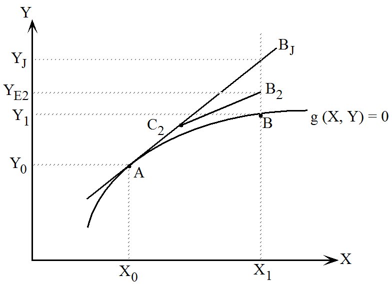
In Euler's method the direction to move at each step is essentially that of the tangent to the curve at the appropriate point. In a 2-step Euler solution (see Figure above), we first go half way along this tangent to point C2, then recompute the direction in which to move, and eventually reach point B2, giving solution YE2. The exact solution is at B where Y has value Y1. In a 4-step Euler simulation we follow a path of 4 straight-line segments, and so on for more steps.
The default method used by GEMPACK is Gragg's method which uses an even more accurate method than Euler's method for calculating the direction in which to move at each step. When the shocks are broken into N parts, Euler's method does N separate calculations while Gragg's method does N+1. Usually the computational cost of this extra calculation is more than repaid by the extra accuracy obtained. More information about Gragg's method (and the similar midpoint method) can be found in section 30.2.
So one way of increasing accuracy is to increase the number of steps. It turns out, however, that the best way to obtain an accurate solution is to carry out 2 or 3 different multi-step calculations with different numbers of steps and to then calculate the solution as an appropriate weighted average of these. This is what is meant by the extrapolated solution.
To illustrate this, we have shown below the different results for the percentage change in household expenditure 'p_Y' in the Stylized Johansen model for the simulation in section 3.1 above, in which labor supply is increased by 10 per cent and capital remains in fixed supply. The table below shows Euler and Gragg results for different step numbers and extrapolations based on them. Note that the exact result is 5.88528.
Multi-step results for different methods and step numbers
   Method     Number of steps
                1         2         4          6        100
    Euler    6.00000   5.94286   5.91412    5.90452    5.88644
    Gragg    5.89091   5.88675   5.88545    5.88529
Extrapolated results
    From Euler 1,2-step results        5.88571
    From Euler 1,2,4-step results      5.88527
    From Gragg 2,4,6-step results      5.88529
Note that, in this case,
- the 4-step Gragg result is more accurate than the 100-step Euler result, and
- the result extrapolated from 1,2,4-step Euler results is much more accurate than the 100-step Euler result (even though the latter takes about 100/7 times as long to compute).
These results are typical of what happens in general.
The general messages are:
- Gragg's method is usually much more accurate than Euler's (for the same number of steps).
- If in doubt, extrapolate.
- Extrapolating from 3 different solutions is better than from 2. For example, extrapolating from Gragg 2,4 and 6-step solutions is usually better than from just 4 and 6-step solutions.
When you extrapolate, if you ask for an Extrapolation Accuracy file (or .XAC file)20, this file shows how accurate the solution is for each endogenous variable. The separate columns show the results for the different multi-step solutions calculated, and the last column of results is the extrapolated result. When you extrapolate from 3 different multi-step results (which is what we recommend), the last two columns give conservative information about the accuracy of each result. (If they show M figures agreement, this means that the 2 different extrapolations based respectively on just the first two and just the first and third agree to this number of figures.)
For example, for the 1,2,4-step Euler results for household expenditure 'p_Y' reported above for the SJLB.CMF simulation (see sections 3.4), the relevant line in the Extrapolation Accuracy file would21 be
p_Y 1 6.00000 5.94286 5.91412 5.88527 CX 4 L5
The results are the 1,2,4-step results and the extrapolation based on them. The comment "CX 4" is an abbreviation meaning that you can have confidence in the extrapolated result (this is the 'CX') and that the two extrapolations (the first based just on the 1,2-step results and the second based on the 2,4-step results) agree to 4 figures (or more). Note that the agreements are reported as figures, not decimal places. (For example 123.4567 and 123.4014 agree to 4 figures, but only one decimal place.) The abbreviations (such as 'CX') used on this file are explained at the top of the file. (The first "1" in the line displayed above means that this line refers to the first - in this case, the only - component of variable p_Y.) The "L5" at the end of this line means that you can be confident of 5 figures accuracy in the level of income Y. [See section 26.2.1 for more details.]
At the end of the file is a summary (we refer to it as the Extrapolation Accuracy Summary) which states how many components fall into each category (EMA, CX etc). For a simulation with Stylized Johansen, this may look something like that shown below.
SUMMARY OF CONVERGENCE RESULTS                 Number  Min Figs Agree
      ------------------------------           ------  --------------
 EMA  Last two results equal to machine accuracy  3         6
 FC0  Fair confidence that the result is zero     2
 CX   Confidence in the extrapolated result      22         2
   2 results are judged accurate to 2 figures.
   4 results are judged accurate to 3 figures.
   16 results are judged accurate to 4 figures.
   3 results are judged accurate to 6 figures.

  Above is for linearised variables.
  Below are for levels values of percent-change and change results.

   1 results are judged accurate to 4 figures.
   21 results are judged accurate to 5 figures.
   5 results are judged accurate to 6 figures.

    (The summary above covers the XAC-retained variables.)
The first part is a summary of the number of times different comments (in the example above, "EMA", "FC0" and "CX") have been used for the different results. The second part tells how many results (linearised, then levels) have been judged accurate to different numbers of figures.
More details about Extrapolation Accuracy Summaries and Extrapolation Accuracy files are given in section 26.2.
The only restriction on step numbers is that, for Gragg's method and the midpoint method, the step numbers must either be all odd or all even (for example, 2,4,6 or 3,5,7). Note also that a 1-step Gragg or midpoint is a little unusual and is probably best avoided (since it is more like Euler than Gragg or midpoint).
More details are given in section 30.2 and some of the theory behind multi-step methods can be found in Pearson (1991).
3.12.3.1 Extrapolation formula for 3 Euler simulations [extrapformula]
As an example, suppose we ran 3 Euler simulations with n1, n2 and n3 steps, yielding (for some variable) solution values of s1, s2 and s3, respectively. Then the extrapolated result E can be calculated as a weighted average of s1, s2 and s3:
E = W1*s1 + W2*s2 + W3*s3
where the weights add to 1. The formula for W1, W2 and W3 are:
W1 = n1*n1*(n3-n2)/denom;
W2 = n2*n2*(n1-n3)/denom;
W3 = n3*n3*(n2-n1)/denom;
where denom:=(n3-n1)*(n2-n1)*(n3-n2);
Some example numbers are given in the table below. Note that W2 is negative.
Table 3.5 Extrapolation weights for 3 Euler simulations
| n1 | n2 | n3 | Total | |
| Steps: | 4 | 8 | 16 | |
| Weights: | 0.333 | -2.000 | 2.667 | 1.000 |
| Steps: | 8 | 16 | 32 | |
| Weights: | 0.333 | -2.000 | 2.667 | 1.000 |
| Steps: | 10 | 20 | 30 | |
| Weights: | 0.500 | -4.000 | 4.500 | 1.000 |
| Steps: | 15 | 20 | 25 | |
| Weights: | 4.500 | -16.000 | 12.500 | 1.000 |
| Steps: | 99 | 100 | 101 | |
| Weights: | 4900.500 | -10000.000 | 5100.500 | 1.000 |
3.12.4 Smiling or frowning face numbers are reported [gpd5.9.2.1]
If you use WinGEM, RunGEM or RunGTAP, you know that after each simulation is completed, you see smiling or frowning faces which indicate how accurately the simulation was solved (provided that you are extrapolating from 3 multi-step calculations). Within ViewSOL, the accuracy summary can be displayed via an icon:

on the upper toolbar.
At the end of the simulation, and at the end of each subinterval if there is more than one, GEMSIM and TABLO-generated programs report (to the terminal and to the LOG file) the face number (between 1 and 10, where 10 is accurate and 1 is very inaccurate). Separate face numbers are shown for the variable and the data accuracy. If there is more than one subinterval, the face number for the overall variable accuracy is shown at the end of the Overall Accuracy Summary (see section 26.3.1).
3.12.5 Fatal error if accuracy too low (GEMSIM and TG-programs) [gpd5.9.2.2]
Suppose that you are extrapolating from 3 multi-step calculations. If the accuracy is extremely low, it is highly unlikely that the simulation results are of any value. Accordingly, the program stops with a fatal error in order to draw your attention to this poor accuracy (but the solution file is still saved).
This can happen at the end of the whole simulation, or it can happen at the end of any subinterval which is solved inaccurately. However it does not happen at the end of a subinterval if you are using automatic accuracy since then you may redo the subinterval in question.
We believe it is your responsibility to decide whether or not a simulation has been solved sufficiently accurately. You should always look at the information provided by the software, especially the Accuracy Summaries (see sections 26.2 and 26.3.1). We are reluctant to intervene and, as when equations are not satisfied very accurately (see section 30.6.1), we end with a fatal error only in what we consider are extreme cases. At present, if any of the face numbers is 3 or less, we stop with a fatal error. Choosing 3 here does not mean that we think face numbers 4,5 and 6 are ok (since often they will not be) - rather we leave the decision to you in such cases.
3.13 GEMPACK programs - an overview [gpd1.2.14]
As you have already seen, GEMPACK is not a single program. There are a number of different programs making up GEMPACK. In this section we give a brief overview of these different programs, grouped by task.
You have not yet used all of the programs below. As you become more experienced with GEMPACK, you may need to come back to this section to check out those programs you have not used.
3.13.1 Working with TABLO input files [gpd1.2.14.1]
TABmate is a special editor for TABLO Input (TAB) files. Use TABmate to create and modify the theory of a model - that is, the TABLO Input file for the model.
TABLO converts the model TAB file into a TABLO-generated program or Auxiliary files for GEMSIM. You must do this before you can carry out a simulation with a model. [See Step 1 in section 3.6.]
In fact TABmate runs the program TABLO in the background. So TABmate and TABLO can perform very similar functions. You can use either TABLO or TABmate to carry out Step 1 for simulations (see section 3.6).
3.13.2 Carrying out simulations [gpd1.2.14.2]
You can use either GEMSIM or the relevant TABLO-generated program to carry out Step 2 for simulations (see section 3.6). Which you use depends on how you ran TABLO in Step 1 (see section 3.6.1 or 3.6.2 above).
GEMSIM. Run GEMSIM to carry out a simulation. Specify the Auxiliary files, starting data files, closure and shocks in a Command file.
TABLO-generated program. Run the EXE file of the TABLO-generated program to carry out a simulation. Specify the starting data files, closure and shocks in a Command file. You can only create TABLO-generated programs if you have a Source-code version of GEMPACK.
3.13.3 Looking at, and processing, simulation results [gpd1.2.14.3]
ViewSOL is for looking at results — see Step 3 in section 3.6.
AnalyseGE is for analysing simulation results. You can view model equations, simulation results and the values of items in the data base. Section 36.6 introduces AnalyseGE. A hands-on introduction to AnalyseGE in the context of a simulation with Stylized Johansen can be found in section 46.1.
SLTOHT is a command-line program that converts simulation results (on a Solution file) either (a) into tables of results which you can import into a spreadsheet, or (b) into a Header Array file. See section 3.10 above and chapters 39 and 40 for information about SLTOHT.
When you report simulation results, you will probably use other standard tools (including spreadsheet programs such as Excel) for making tables and graphs.
3.13.4 Working with data [gpd1.2.14.4]
In GEMPACK data for models are usually held on Header Array files. Because these are binary (ie, non-text) files, you need special programs to work with the data in this form.
ViewHAR is for looking at data on Header Array files. You used ViewHAR to look at original and updated data in the Stylized Johansen example above. ViewHAR can also be used to create a Header Array file and to modify data on a Header Array file (see section 6.1 below and section 6.2).
CMPHAR can be used to compare the data on two Header Array files — see section 37.2.
CMBHAR can be used to combine the data on two or more Header Array files (for example, data representing two or more years). See section 37.3.
Data comes from various sources. You may use other standard tools and programs (including spreadsheet programs such as Excel) when working with data.
3.13.5 Windows modelling environments [gpd1.2.14.5]
WinGEM provides a Windows environment for carrying out modelling and associated tasks.
RunGEM provides a Windows environment for carrying out simulations with a fixed model. Users with little experience of modelling can carry out simulations by choosing just the closure and shocks. See section 36.5 and chapter 45.
RunDynam and variants including RunGDyn are sold as as a separate product. They are Windows interfaces for use with recursive dynamic models such as USAGE and dynamic GTAP. See section 36.7.
3.13.6 Other programs for special tasks [gpd1.2.14.6]
These are programs used for specialised tasks, usually by power users. You will not need to use any of them until you are more experienced with GEMPACK.
ACCUM and DEVIA are used for working with recursive dynamic models such as USAGE which are solved annually over a period of several years. ACCUM and DEVIA collect the results for several years. [See chapter 41.]
SUMEQ is for looking at data on an Equations file. SUMEQ can also be used to diagnose homogeneity problems with a model — see chapter 79.
SEENV is for working with Environment files (which store the set of exogenous and endogenous variables in one closure for a model) — see chapter 56.
3.13.7 Programs for use on non-Windows PCs [gpd1.2.14.7]
Windows programs, such as WinGEM, ViewHAR or ViewSOL, will not run on non-Windows PCs22 -- so other, command-line programs are needed to turn data (HAR) and results (SL4) files into text files that you can view. These are:
SEEHAR turns a Header Array file into a viewable text file — see section 37.1.
3.14 Different GEMPACK files [gpd1.2.15]
As you have seen, GEMPACK programs produce and use several different types of files (for example, Solution files and Header Array files). New users often ask us "Why are there so many different files?".
In this section we give more details about these different files and how they are used.
In our experience, some users are keen to have detailed information about this topic while others are not very interested. Since a detailed knowledge about this topic is not essential for doing effective modelling, you should feel free to skip this section or to skim it very quickly. You can always refer back to it later on, if and when you need to.
A table summarising the different files is given in section 3.14.6 below.
3.14.1 The most important files [gpd1.2.15.1]
We begin with the most important files, namely TABLO Input files, data files, Command files and Solution files, all of which you have met earlier in this chapter.
TABLO Input files. These contain the theory (equations etc) for a model. Alternatively they may be for data manipulation. These files have suffix .TAB. These files are inputs to the program TABLO. The program TABmate (see section 36.4) can be used to create and or modify these files.
Data files. These may be Header Array files or text files. The suffix is not prescribed by the software, though suffix .HAR is recommended (.DAT is sometimes used). Data files can be inputs to a simulation (the original input-output data, the parameters) and updated versions are output from a simulation. Updated data files are usually given the suffix .UPD . Chapter 6 below contains an introduction to the different ways in which you can create data files and modify data on existing data files.
Command files. These contain the details of a simulation, including closure, shocks, starting data and solution method (see section 3.8). The suffix is not prescribed by the software, though .CMF is usual23. Command files are inputs for GEMSIM and TABLO-generated programs. The statements allowed in Command files are documented in chapter 35.
Solution files. These are the main outputs from a simulation. They contain the change or percentage change results for all the linearized variables. They may also contain levels results. These files have suffix .SL4. They are inputs to various post-simulation programs such as ViewSOL, SLTOHT, and AnalyseGE. Solution files are documented in chapter 27.
Equations files. These contain numerical versions of the linearized equations of a model. They are usually only produced when you wish to use SAGEM to obtain several Johansen (approximate) solutions of a model, as explained in chapter 58. You may also create an Equations file if your model is not homogeneous in prices or quantities (see section 79.1). Equations files have suffix .EQ4. Equations files are documented in chapter 59.
Shock files. Sometimes it is necessary to shock the different components of a variable by different amounts. If the variable has a large number of components, or if the shocks are calculated by a program, it is convenient to put the numerical values of the shocks onto a so-called "shocks file". This file may be a text file or a Header Array file. The suffix for shocks files is not prescribed by the software, though often .SHK is used. The use of shock files is documented in sections 24 to 66.2.
Solution Coefficients (SLC) files. These are output from a simulation. They contain the pre-simulation values of all data and of all Coefficients in the TABLO Input file for the model. These files have suffix .SLC and have the same name (apart from suffix) as the Solution file from the simulation24. The program AnalyseGE reads both the Solution and SLC file when you analyse the results of a simulation25. You can also examine SLC files with ViewHAR. SLC files are documented in section 28.1.
Extrapolation Accuracy files. You can ask26 for an Extrapolation Accuracy file to be produced when you extrapolate from 3 separate multi-step calculations (as you have seen in section 3.12.3 above). These text files show estimates as to how accurate the different simulation results are. They have suffix .XAC and have the same name (apart from suffix) as the Solution file from the simulation. Extrapolation Accuracy files are documented in section 26.2.
3.14.2 Files for communication between programs [gpd1.2.15.2]
There are a number of files which are used for communication between programs. The most important of these are the Auxiliary files which allow communication between TABLO and GEMSIM or the TABLO-generated program.
Auxiliary files. These are either
- Auxiliary files for a TABLO-generated program. These are produced when TABLO writes a TABLO-generated program (see section 3.6.1 above). These files have suffix .AXS (Auxiliary Statement file) and .AXT (Auxiliary Table file).
- GEMSIM Auxiliary files. These are produced when TABLO writes output for GEMSIM (see section 3.6.2 above). These files have suffix .GSS (GEMSIM Statement file) and .GST (GEMSIM Table file).
TABLO-generated program (Fortran file). This is the Fortran (.FOR) file for the TABLO-generated program which is produced by TABLO (see section 3.6.1 above). Auxiliary files (.AXS and .AXT files) are always produced at the same time. In Step 1(b) for simulations (see section 3.6.1), this program is compiled and linked to produce the EXE file of the TABLO-generated program27. It is this EXE file which is run to carry out a simulation.
When the EXE file of a TABLO-generated program is used to carry out a simulation, the Auxiliary files (AXS and AXT files) are required. They communicate vital information from the TABLO Input file to the simulation.
Similarly, if GEMSIM is used to carry out a simulation, the GEMSIM Auxiliary files (GSS and GST files) are required.
3.14.3 LOG files [gpd1.2.15.3]
Often a program runs very quickly and/or puts a lot of information on the screen. If you need to check this output (for example, to see where an error occurs), you can ask for a LOG file to be created28. You can then look at this log file in your favourite text editor. The suffix for LOG files is not prescribed by the software, though suffix .LOG is usual.
3.14.4 Stored-input (STI) files [gpd1.2.15.4]
These days, GEMPACK Windows programs such as TABmate, RunDynam or WinGEM are the main interface seen by most GEMPACK users — but a lot of the work they seem to perform is in fact carried out by command-line programs running in the background.
In previous times, before the GEMPACK Windows programs were available, GEMPACK users usually ran programs like TABLO, GEMSIM and SLTOHT from the command line. The program would ask a sequence of questions — the responses were usually single letters (to indicate options) or filenames (for input and output).
Obviously it could be very tedious to repeatedly run programs in this way. Stored-input files or STI files were a way to reduce the drudgery — they consist of a text file which stores the necessary responses to the questions that the program asked. Then, to repeat an SLTOHT job, one merely typed, say:
sltoht -sti report3.sti
where report3.sti is a text file of the responses needed to generate some report. To produce report3.sti you would, the first time you ran this job, either note responses on a scrap of paper (the old way) or activate the SIF option in SLTOHT which will record your responses in a file.
STI files are rather hard to read and understand — you only see one half of a conversation.
For modern GEMPACK users the most-frequently encountered STI files may be those used for input to TABLO which specify the condensation (section 14.1.2 gives an example). For new models you can and should specify condensation actions — such as Omit, Substitute and BackSolve — within the TAB file, but this option is relatively new, so many older models still use a STI file to store the condensation.
Apart from this, the main remaining uses of STI files are:
- to automate the running of SLTOHT or some other command-line programs which need to be run repeatedly
- to activate some rarely used options in TABLO or other programs. A few options are only accessible via STI files (or by direct responses to program queries).
Stored-input files are further described in section 48.3. They usually have suffix .STI (although other suffixes may be used). You will need to learn about STI files as you become more experienced. You can find introductory examples of creating and working with them in sections 14.1.2, 14.1.4 and 54.11.
3.14.5 Files for power users [gpd1.2.15.5]
A number of files can be created in order to speed up or simplify subsequent tasks. These are typically used mainly by experienced GEMPACK users so you don't need to know any details about them at this stage. Examples are Stored-input files (see section 3.14.4 above), Environment files (see section 23.2) and various Mapping files (see sections 39.3, 39.8 and 40.1).
3.14.6 Summary of files [gpd1.2.15.7]
Table 3.6 Summary of the different files
| File Type and Suffix | Input to | Output from |
| TABLO Input file (TAB) | TABLO, TABmate | TABmate |
| Data files (often HAR) | Simulations, Data-manipulation TAB files, ViewHAR, CMBHAR, SEEHAR etc | Simulations, Data-manipulation TAB files,ViewHAR, SLTOHT etc |
| Command files (usually CMF) | TABLO-generated programs, GEMSIM, SAGEM | text editor |
| Solution files (SL4) | ViewSOL, ViewHAR, AnalyseGE, SLTOHT | TABLO-generated programs, GEMSIM, SAGEM |
| Equations files (EQ4) | SAGEM, SUMEQ | TABLO-generated programs, GEMSIM |
| Shock files (often SHK) | TABLO-generated programs, GEMSIM, SAGEM | text editor, TABLO-generated programs, GEMSIM |
| SLC files (SLC) | AnalyseGE | TABLO-generated programs and GEMSIM |
| Extrapolation Accuracy files (XAC) | TABLO-generated programs and GEMSIM | |
| Auxiliary files (GSS/GST or AXS/AXT) | GEMSIM or TABLO-generated program | TABLO |
| TABLO-generated Fortran program (FOR) | Compile and link - Step 1(b) in section 3.6.1 | TABLO |
| LOG files (usually LOG) | Any command-line GEMPACK program | |
| Stored-input files (usually STI or SIF) | Any command-line GEMPACK program | Text editor, or any GEMPACK program (see options SIF and ASI in section 48.3). |
3.14.7 Work files [gpd1.2.15.6]
Many programs create and use working files while they are running. These work files can be large. Usually these work files are deleted when the program finishes so you do not see them or need to know about them. Occasionally these files are left around on your hard disk if the program finishes with an error. See below or section 30.7 for more details.
3.14.8 Files you can eventually delete [junkfiles]
Especially when running multiperiod simulations, GEMPACK tends to create many output files — most of which will not be needed in a few days time. A list of these 'junk files' appear below. A command-line program, GPDEL, is provided, which will remove many of these files. From a command prompt in your working folder, type:
GPDEL
to see instructions for using it. Alternatively, TABmate's Tools..Delete Junk files menu item offers another way to cull files.
Table 3.7 Files you can eventually delete
| Filename pattern | Description |
| *.BAK | Backups of files modified by TABmate and ViewHAR |
| *.LOG | Log files made by many GEMPACK programs |
| *.MDV *.MDC *.MDE | Tables of variables, coefficients and equations made by TABmate |
| *.CLO | Closure report from TABmate |
| *.INF *.MNC | Output from TABLO |
| *.TBR *.TBT | Temporary files made by TABLO |
| *.UD3 *.UD4 *.UD5 *.UD6 *.UD7 *.UD8 *.UD9 | Temporary files of updated coefficients produced during a simulation |
| *assert-fail.har | Diagnostic files produced when an assertion fails |
| *assert-arith-fail.har | Diagnostic files produced when there is an arithmetic error or overflow |
| *.CWK *.DWK *.IWK *.PWK *.SWK *.E2K *.EXS *.EL2 *.RDT | Temporary work files produced during a simulation — usually only visible if a simulation crashes. |
| *.SLC *.UDC *.AVC *.CVL | Files of coefficient values produced mainly for use by AnalyseGE, details here. |
| optin_1 optin_2 opt80 opt80_2 parcomp.* | Temporary files produced while compiling TABLO-generated Fortran programs |
3.15 For new users - what next? [gpd1.2.16]
Congratulations. You have just learnt the most important things about GEMPACK, namely how to set up and carry out simulations, and how to look at the results.
Where you go next in learning about GEMPACK depends on your main purpose in using the software.
- If you mainly want to carry out simulations with another standard model, you will find a list of the models supplied with GEMPACK in section 1.5. If the model you wish to work with is one of these, you will find detailed hands-on guidance in chapter 43 about carrying out standard simulations with many of these models. If you wish to work with another model, the model developers have probably supplied and documented one or more standard simulations. We suggest that you start with those.
- With a well-documented model and good software, it is relatively easy to carry out simulations and produce, and report, a large number of results. It is less easy to really understand these results. The GEMPACK program AnalyseGE (see section 36.6) provides valuable assistance to you in this task. You can find a hands-on introduction to AnalyseGE in the context of a Stylized Johansen simulation in section 46.1. Pearson et al. (2002) provides a hands-on introduction to AnalyseGE in the context of simulations with GTAP. We encourage you to explore the use of AnalyseGE as you analyse the results of simulations you carry out.
- If you want to build your own model (or modify someone else's), or if you just want to understand how a model is implemented in GEMPACK, you should read chapter 4. Perhaps read it quickly the first time and then go back for a more detailed study.
- If you need to build or modify the data files for a model, you should read chapter 6.
- When you want to know more about the GEMPACK utility programs (say, for report generation or post-simulation processing of results), look at the detailed documentation in Chapters 36 to 40.
- When you want to know more about running the GEMPACK programs, read chapter 48. This chapter gives detailed suggestions for more efficient use of the programs whether you are running them interactively or in batch mode.
Whatever your main interest, we strongly encourage you to at least skim chapter 4 first, and then go on to your main interest. You must be familiar with at least the basics of TABLO Input (TAB) files in order to work properly with, and understand, any model implemented via GEMPACK.
4 Building or modifying models [gpd1.3]
Click here for detailed chapter contents
In order to build a model within GEMPACK, it is necessary to prepare a TABLO Input file containing the equations of the model and to construct one or more data files whose purpose is essentially to give one solution of the levels equations of the model.
The preparation of a TABLO Input file involves
- writing down the equations in a suitable form. You can use levels equations, linearized equations or a mixture of these. We discuss this in section 4.1 below.
- working out the data requirements of the model. This is discussed in section 4.2 below.
We describe the preparation of TABLO Input files in section 4.3 and the preparation of the actual data files in chapter 6. We illustrate each step in the process by doing it for the Stylized Johansen model.
Of course, to modify an existing model, you modify the TABLO Input file (to change the theory of the model) and/or the data file(s).
The TABLO Input file given for Stylized Johansen in section 4.3.3 is a mixed one (in the sense that it contains a mixture of linearized and levels equations). In sections 4.4.1 and 4.5.1 we describe alternative TABLO Input files for Stylized Johansen consisting only of linearized or levels equations respectively.
TABLO linearizes all levels equations in TABLO Input files and converts all levels variables to the associated linear ones (change or percentage change in the associated levels variables). This is described in section 4.6.
We conclude this chapter in section 4.7 where we give you advice about building your own model by writing a TABLO Input file from scratch or by modifying an existing one. We include hands-on examples showing how to identify and correct errors in TABLO Input files and Command files.
If you are familiar with using GAMS for general equilibrium modelling, you may prefer to work through the document Kohlhaas and Pearson (2002) instead of, or before, reading this chapter. The many similarities between GEMPACK and GAMS make it relatively easy for a GAMS modeller to begin using GEMPACK productively.
Table 4.1 Levels and linearized equations of the Stylized Johansen model
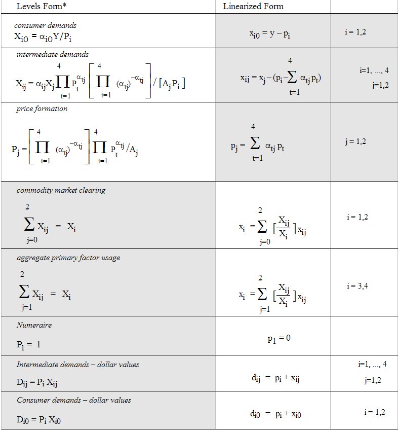
In Table 4.1, upper-case Roman letters represent the levels of the variables; lower-case Roman letters are the corresponding percentage changes (which are the variables of the linearized version shown in the second column). The letters P, X and D denote prices, quantities and dollar values respectively, while the symbols A and a denote parameters. Subscripts 1 and 2 refer to the (single) commodities produced by industries 1 and 2 (subscript i), or to the industries themselves (subscript j); i = 3 refers to labour while i = 4 refers to the model's one (mobile-between-industries) type of capital; subscript j = 0 identifies consumption. Because the first three equation blocks are identically linear in the logarithms they are natural candidates for presentation and explanation of the model.
4.1 Writing down the equations of a model [gpd1.3.1]
TABLO Input files contain the equations of a model written down in a syntax which is very similar to ordinary algebra. Once you have written down the equations of your model in ordinary algebra, it is a simple matter to put them into a TABLO Input file, as we illustrate in section 3.3 below.
You are free to use levels or linearized versions of the equations or a mixture of these two types. For example, if a certain dollar value D is the product of the price P and quantity Q, the levels equation is
D = P * Q
(where the "*" indicates multiplication), and the associated linearized equation is
p_D = p_P + p_Q
where "p_" denotes "percentage change in". The linearized version says that, to first order of approximation, the percentage-change in the dollar value is the sum of the percentage changes in the price and the quantity. Whichever version of the equation you include, GEMPACK can still produce accurate solutions of the underlying levels equations (which are usually nonlinear).
We say more about the process of linearizing equations in section 3.7 below.
The best way of making the above clear is to take a concrete example, as we do below, using Stylized Johansen as our example model.
4.1.1 Writing down the equations of Stylized Johansen [gpd1.3.1.1]
We start from the equations as written down in Chapter 3 of DPPW (to which we refer readers interested in the derivation of, and motivation behind, these equations). An excerpt from that chapter, SJ.PDF, is included in the "examples" subfolder of your GEMPACK directory.
The equations of the model are shown in Table 4.1. In that table, both the levels and linearized versions of each equation are shown, taken essentially unchanged from DPPW1. Notice that upper case letters (for example, X) denote levels quantities while lower case letters (for example, x) denote percentage change in the corresponding levels quantity.
For our first implementation of Stylized Johansen (see section 4.3 below), we have chosen a mixed representation, based on the shaded blocks in Table 4.1. That is, we decided to use the levels versions of some of the equations (most are accounting identities and one is the numeraire equation) and the linearized versions of the top three equations (which are behavioural equations). Later, in sections 4.4 and 4.5 respectively, we describe implementations based on exclusively linearized equations (section 4.4) and exclusively levels equations (section 4.5). Of course, each of these 3 implementations is valid and all three produce the same results.
The notation in DPPW involves a liberal use of subscripts which are not suitable for the linear type of input usually required by computers (and required in the TABLO Input file). Hence we use a different notation. The levels variables of the model are as follows. In DPPW subscripts 1 and 2 refer to sectors (commodity or industry), subscripts 3 and 4 refer to factors (3 is labor and 4 is capital) while subscript 0 refers to households.
Table 4.2 Levels variables for Stylized Johansen
| GEMPACK variable | Meaning | DPPW | Notation |
| Y | Value of household income | Y | |
| PC(i) | Price of commodity i | Pi | (i=1,2) |
| PF(f) | Price of factor f | Pf | (f=3,4) |
| XCOM(i) | Supply of commodity i | Xi | (i=1,2) |
| XFAC(f) | Supply of factor f | Xf | (f=3,4) |
| XH(i) | Household use of commodity i | Xi0 | (i=1,2) |
| XC(i,j) | Intermediate input of commodity i to industry j | Xij | (i,j=1,2) |
| XF(f,j) | Input of factor f to industry j | Xfj | (f=3,4;j=1,2) |
| DVCOMIN(i,j) | Dollar values for intermediate inputs | (i,j=1,2) | |
| DVFACIN(f,j) | Dollar values for factor use by industry | (f=3,4;j=1,2) | |
| DVHOUS(i) | Dollar values for household consumption | (i=1,2) |
Table 4.3 Parameters for Stylized Johansen levels equations
| Parameters | Description | DPPW | Notation |
| ALPHACOM(i,j) | Commodity exponents in production function for sector j (E3.1.4) | ALPHAij | (i,j=1,2) |
| ALPHAFAC(i,j) | Factor exponents in production function for sector j (E3.1.4) | ALPHAfj | (f=3,4; j=1,2) |
We introduce sets SECT, the set of two sectors say "s1" and "s2", and FAC, the set of the two factors "labor" and "capital".
Below in Table 4.4, we have rewritten the selected equations from Table 4.1, this time using the GEMPACK variables and notation as in Tables 4.2 and 4.3. Note that below we also use the GEMPACK convention that "p_" indicates percentage change in the relevant levels variable. For example, p_XH(i) denotes the percentage change in XH(i), household consumption of commodity i. In these equations we use "*" to denote multiplication and "/" to denote division. We also use SUM(i,<set>,<expression>) to denote sums (usually expressed via Greek sigma) over all i in the set <set>; here <set> is SECT or FAC.
Note that below we also use the GEMPACK convention that "p_" indicates percentage change in the relevant levels variable. For example, p_XH(i) denotes the percentage change in XH(i), household consumption of commodity i. In these equations we use "*" to denote multiplication and "/" to denote division. We also use SUM(i,<set>,<expression>) to denote sums (usually expressed via Greek sigma) over all i in the set <set>; here <set> is SECT or FAC.
Table 4.4 Stylized Johansen equations in GEMPACK notation
        Equation                                      Subscripts         No. in DPPW
(E1)  p_XH(i)   = p_Y - p_PC(i)                       i in SECT          E3.2.1
(E2)  p_XC(i,j) = p_XCOM(j) - [p_PC(i) - p_PC(j)]     i,j in SECT        E3.2.2, E3.2.3
(E3)  p_XF(f,j) = p_XCOM(j) - [p_PF(f) - p_PC(j)]     f in FAC,j in SECT E3.2.2, E3.2.3
(E4)  p_PC(j)   = SUM(i,SECT, ALPHACOM(i,j)*p_PC(i))
                + SUM(f,FAC,  ALPHAFAC(f,j)*p_PF(f))  j in SECT          E3.2.3
(E5)  XCOM(i)   = XH(i) + SUM(j,SECT, XC(i,j))        i in SECT          E3.1.6
(E6)  XFAC(f)   = SUM(j,SECT, XF(f,j))                f in FAC           E3.1.7
(E7)  PC("s1")  = 1.                                                     E3.1.23
(E8)  XC(i,j)   = DVCOMIN(i,j) / PC(i)                i,j in SECT           -
(E9)  XH(i)     = DVHOUS(i) / PC(i)                   i in SECT             -
(E10) XF(f,j)   = DVFACIN(f,j) / PF(f)                f in FAC, j in SECT   -
These equations appear essentially as above in the TABLO Input file (see section 4.3.3 below).
4.2 Data requirements for the linearized equations [gpd1.3.2]
As a general rule, GEMPACK requires an initial levels solution of the model. Thus it is necessary to provide data from which initial (that is, pre-simulation) values of all levels variables and the values of all parameters of the model can be inferred. As we shall see in section 4.2.1 for Stylized Johansen, it is frequently the case that the data required are
- mainly dollar values (rather than separate prices and quantities), and
- certain parameters (such as elasticities).
Once dollar values are known, it is often possible to set basic prices equal to 1 (this amounts to a choice of units for the related quantities), from which the quantities can be derived by dividing the dollar value by the price. [The choice of 1 for the basic price is, of course, arbitrary. Any other fixed value would be as good.]
4.2.1 Data requirements for Stylized Johansen [gpd1.3.2.1]
Suppose that we know the following pre-simulation dollar values.
DVCOMIN(i,j)    Intermediate inputs
DVHOUS(i)       Household consumption
DVFACIN(f,j)    Factor use by industry
Then, if we set all the prices to one for
PC(i)           Price of commodities
PF(f)           Price of factors
we can infer all other levels variables in Table 4.2 as follows.
XC(i,j) = DVCOMIN(i,j) / PC(i)      Intermediate inputs
XH(i)   = DVHOUS(i) / PC(i)         Household use
XF(f,j) = DVFACIN(i,j) / PF(f)      Factor use
Y       = SUM(i, SECT, DVHOUS(i))   Household expenditure
The only other quantities in the equations (E1)-(E10) are the parameters ALPHACOM(i,j) and ALPHAFAC(f,j) in (E4). Because there is a Cobb-Douglas production function involved, it is well-known that these are cost shares, namely
ALPHACOM(i,j) = DVCOMIN(i,j) / DVCOSTS(j),
ALPHAFAC(f,j) = DVFACIN(f,j) / DVCOSTS(j),
where DVCOSTS(j) is an abbreviation for
SUM(i, SECT, DVCOMIN(i,j)) + SUM(f, FAC, DVFACIN(f,j)),
the total costs in industry j. [These results are easily obtained from equations (E3.1.10) and (E3.1.12) in DPPW.]
Thus the only data requirements are the dollar values
DVHOUS(i), DVCOMIN(i,j) and DVFACIN(f,j)
One instance of the data required is as shown in the body of Table 3.1 in section 3.1.1 above.
In the TABLO Input file, the pre-simulation values of these data will be read and the values of all others will be calculated from them.
4.3 Constructing the TABLO input file for a model [gpd1.3.3]
The TABLO Input file of the model is the means of communicating the theory of the model to the computer, in particular to the GEMPACK program TABLO. It consists of the equations written in a syntax which is very similar to ordinary algebra. It also contains a description of the data to be read, where it is to be read from, and how this data is to be used to calculate values of parameters and pre-simulation values of the other levels variables occurring in the equations.
The main part of a TABLO Input file is the equations, which usually come at the end of the file. Before the equations must come
- the VARIABLEs (levels or linearized);
- the SETs used to describe the different arguments of variables;
- the data to be read;
- calculations of the pre-simulation values of any levels variables not read in as data (calculations are done via FORMULAs);
- calculations (via FORMULAs) of any parameters whose values are not read in;
- logical names of the associated data files;
- the headers on the data file(s) where the different pieces of data are to be found (if the data files are GEMPACK Header Array files — see chapter 5).
The order of these in the TABLO Input file is somewhat flexible but follows the general rule that items cannot be used until they have been declared. Thus the SET statements (saying which sets are involved) usually come first. Then the declarations of data files (via FILE statements) often come next, followed by the declarations of the VARIABLEs and parameters.
These ideas are best learnt and understood by example. Hence we launch straight into the preparation of the TABLO Input file for Stylized Johansen.
4.3.1 Viewing the TABLO input file [gpd1.3.3.1]
When working with GEMPACK, many of the input files that you create are text files, so you need a text editor. You can use any text editor you are familiar with.
GEMPACK includes two text editors, TABmate and GemEdit. We suggest you use TABmate since it has coloured highlighting of TABLO syntax, and a powerful Gloss feature which displays all parts of the TABLO code where a chosen variable or coefficient is used. If TABmate is not the default editor in WinGEM, select, in the WinGEM main menu,
Options | Change editor...
then select your editor Use TABmate. You should only have to do this once: WinGEM should remember which editor you chose.
Open the TABLO Input file for Stylized Johansen SJ.TAB in the TABmate editor. In WinGEM, to edit a text file, select in the WinGEM menu,
File | Edit file...
The edit box should show various files in the directory C:\SJ. If the Open box does not start at the correct directory C:\SJ, set the Working directory again as described in section 3.4.2.
Select the file SJ.TAB, the TABLO Input file for the Stylized Johansen model.
Search the TABLO Input file for "EQUATION House" using Search | Find. We will discuss the details of this equation in the next section.
4.3.2 Constructing part of the TABLO input file for Stylized Johansen [gpd1.3.3.2]
In this subsection we consider just two equations of Stylized Johansen, namely (E9) and (E4) in section 4.1.1 above. We show how these are written in the TABLO Input file. (We show the full TABLO Input file in section 4.3.3 and then discuss the rest of this file in section 4.3.4 below.)
Equation (E9)
Consider the very simple equation (E9) relating prices, quantities and dollar values of household consumption.
In the TABLO Input file this equation is written as2
EQUATION House # Household demand for commodity i #
    (all,i,SECT) XH(i) = DVHOUS(i) / PC(i) ;
where
- EQUATION is a keyword indicating that what follows is an equation,
- House is the name by which this equation is known in the model,
- the words between the hashes # form optional additional labelling information which is associated with the equation,
- the quantifier (all,i,SECT) indicates that there are really several equations, one for each sector, and
- the semicolon ; marks the end of this part of the equation statement.
For this equation to be meaningful, we must explain in the TABLO Input file all the names used in the equation.
The levels variables are declared (that is, explained) via the statements
VARIABLE (all,i,SECT) XH(i)  .    # Household demand for commodity i # ;
VARIABLE (all,i,SECT) DVHOUS(i).  # Dollar value of household use of commodity i # ;
VARIABLE (all,i,SECT) PC(i)       # Price of commodity i # ;
Notice that, by convention, these declarations also declare associated linear variables p_XH, p_DVHOUS and p_PC which denote the percentage-change in the relevant levels variables. These linear variable names are used in reporting simulation results (see the results in section 3.7 above, for example) and are available for use in linearized equations in the TABLO Input file (see, for example, the EQUATION named "Price_formation" discussed later in this section) without further explicit declaration.
The fact that SECT is a set with two sectors "s1" and "s2" in it is indicated via the SET statement
SET SECT # Sectors # (s1-s2) ;
We must also indicate how pre-simulation values of the levels variables can be read or calculated from the data base. We do this via the statements
READ DVHOUS  from FILE iodata HEADER "HCON" ;
FORMULA (all,i,SECT)   PC(i) = 1 ;
FORMULA (all,i,SECT)   XH(i) = DVHOUS(i)/PC(i) ;
In the first of the above statements,
- READ is the keyword,
- iodata is the (logical) name by which the particular data file containing this input-output data is known in the TABLO Input file, and
- the Header "HCON" tells where on the file the relevant array of data is to be found.
In the second and third statements, FORMULA is the keyword.
The third of these contains the same expression as the equation we are considering. Indeed, we can combine the EQUATION and FORMULA into a single statement on the TABLO Input file, namely.3
FORMULA & EQUATION House # Household demand for commodity i #
  (all,i,SECT)   XH(i) = DVHOUS(i) / PC(i) ;
The statement
FILE iodata # input-output data for the model # ;
declares "iodata" as the logical name4 of the file containing the actual data.
This ends the discussion of the equation (E9) and of all the statements needed for the EQUATION House.
Using the Gloss feature in TABmate
In TABmate, there is a quick way of finding all places where a name such as XH occurs in the TABLO Input file SJ.TAB. In TABmate, click on TABLO Check in the bar near the top of the TABmate screen5. Click on the word EQUATION in the "EQUATION House" and then click on Gloss in the bar near the top of the TABmate screen. A box (shown below) appears showing all names used in the EQUATION House in the TABLO Input file.
FORMULA & EQUATION House # Household demand for commodity i #
   (all,i,SECT) XH(i) = DVHOUS(i) / PC(i) ;
Line
~41: SET SECT # Sectors # (s1-s2) ;
~69: Coefficient Variable (GE 0) (all,i,SECT) XH(i) # Household demand for commodity i # ;
~86: Coefficient Variable (GE 0) (all,i,SECT) DVHOUS(i)
                                        # Dollar value of household use of commodity i # ;
~59: Coefficient Variable (GE 0) (all,i,SECT) PC(i) # Price of commodity i # ;
Click on the X in the top right-hand corner of the Glossary box to exit from the Gloss box.
Click on the word XH in the "EQUATION House" and then click on the Gloss button. The Gloss box (shown below) appears showing all occurrences of the name XH in the TABLO Input file.
Coefficient   XH
Line
~69: Variable (GE 0) (all,i,SECT) XH(i) # Household demand for commodity i # ;
~138: FORMULA & EQUATION House # Household demand for commodity i #
   (all,i,SECT) XH(i) = DVHOUS(i) / PC(i) ;
~142: FORMULA & EQUATION Com_clear # Commodity market clearing #
   (all,i,SECT) XCOM(i) = XH(i)+SUM(j,SECT,XC(i,j));
Try clicking on the word DVHOUS to see where DVHOUS is used in the TABLO Input file SJ.TAB.
Equation (E4)
Now consider the equation (E4) "price formation for commodities". This is written in the TABLO Input file as
EQUATION (LINEAR) Price_formation
         (all,j,SECT) p_PC(j) = SUM(i,SECT, ALPHACOM(i,j)*p_PC(i)) +
                                SUM(f,FAC,  ALPHAFAC(f,j)*p_PF(f)) ;
in which
- the qualifier (LINEAR) indicates that this is a linearized equation (not a levels equation),
- the fact that p_PC(i) and p_PF(f) are percentage-changes in the levels variables PC(i) and PF(f) is guaranteed by the convention that, once these levels variables have been declared via
VARIABLE (all,i,SECT) PC(i) # Price of commodity i # ;
VARIABLE (all,f,FAC)  PF(f) # Price of factor f # ;
the associated linear variables p_PC(i) and p_PF(f) are automatically considered declared. In this equation, ALPHACOM and ALPHAFAC are parameters. To calculate ALPHACOM and ALPHAFAC from the data base, FORMULA statements are used:
FORMULA  .# Share of intermediate commodity i in costs of industry j #
(all,i,SECT)(all,j,SECT)  ALPHACOM(i,j) = DVCOMIN(i,j) /
    [SUM(ii,SECT,DVCOMIN(ii,j)) + SUM(ff,FAC,DVFACIN(ff,j)) ] ;
FORMULA  .# Share of factor input f in costs of industry j #
(all,f,FAC)(all,j,SECT)  ALPHAFAC(f,j) = DVFACIN(f,j) /
    [SUM(ii,SECT,DVCOMIN(ii,j)) + SUM(ff,FAC,DVFACIN(ff,j)) ] ;
where FORMULA is the keyword. The fact that ALPHACOM and ALPHAFAC are parameters can be indicated via the statements
COEFFICIENT(PARAMETER) (all,i,SECT)(all,j,SECT) ALPHACOM(i,j) ;
COEFFICIENT(PARAMETER) (all,f,FAC) (all,j,SECT) ALPHAFAC(f,j) ;
in which COEFFICIENT is the keyword and (PARAMETER) is a qualifier.
If you are using the TABmate editor, try using the Gloss button. Click on the word p_PC in the EQUATION Price_formation and click on the Gloss button to see all occurrences of p_PC in the TABLO Input file SJ.TAB. Click on the word "FAC" and Gloss to see all occurrences of the set FAC.
This ends the discussion of the equation (E4) and of all the statements needed for the EQUATION Price_formation.
Statements in a TABLO Input File
The main types of statements in a TABLO Input file, namely EQUATIONs, FORMULAs, READs, VARIABLEs, COEFFICIENTs, SETs and FILEs have been introduced in connection with equations House (E9) and Price_formation (E4) above
Each entity (VARIABLE, COEFFICIENT, etc) must be declared in the TABLO Input file before it is used in EQUATIONs and FORMULAs. This partly determines the order of the statements in the TABLO Input file.
We suggest that you now look at the complete TABLO Input file for this model, as set out in section 4.3.3 below, or using the editor TABmate (or your text editor). This file is usually called SJ.TAB when supplied with the GEMPACK Examples. You will find all the statements shown above in that file.
Since declarations must come before use, you will find the TABLO statements in pretty much the reverse order from that in which we have introduced them above.
We discuss the rest of this TABLO Input file in section 4.3.4.6
4.3.3 "Mixed" TABLO input file for the Stylized Johansen model [gpd1.3.3.3]
!-------------------------------------------------------------------!
!                  Mixed TABLO Input file for the                   !
!                    Stylized Johansen model                        !
!                                                                   !
!         following the description in Chapter 3 of the text        !
!   "Notes and Problems in Applied General Equilibrium Economics"   !
!       by P.Dixon, B.Parmenter, A.Powell and P.Wilcoxen [DPPW]     !
!              published by North-Holland 1992.                     !
!                                                                   !
!-------------------------------------------------------------------!
! Text between exclamation marks is a comment.                      !
! Text between hashes (#) is labelling information.                 !
!-------------------------------------------------------------------!
!     Set default values                                            !
!-------------------------------------------------------------------!
VARIABLE (DEFAULT = LEVELS) ;
EQUATION (DEFAULT = LEVELS) ;
COEFFICIENT (DEFAULT = PARAMETER) ;
FORMULA (DEFAULT = INITIAL) ;
!-------------------------------------------------------------------!
!      Sets                                                         !
!-------------------------------------------------------------------!
! Index values i=1,2 in DPPW correspond to the sectors called s1,s2.
  Index values i=3,4 in DPPW correspond to the primary factors,
  labor and capital.   The set SECT below doubles as the set of
  commodities  and the set of industries. !
SET SECT # Sectors # (s1-s2)  ;
SET FAC # Factors  # (labor, capital) ;
SET NUM_SECT # Numeraire sector - sector 1 #  (s1) ;
SUBSET  NUM_SECT is subset of SECT ;
!-------------------------------------------------------------------!
!      Levels variables                                             !
!-------------------------------------------------------------------!
! In the DPPW names shown below, : denotes subscript.               !
! For example, x:j indicates that j is a subscript.                 !
VARIABLE               Y    # Total nominal household expenditure #
                              ! This is also Y in DPPW ! ;
VARIABLE (all,i,SECT)  PC(i)   # Price of commodity i #
                                ! This is p:i (i=1,2) in DPPW ! ;
VARIABLE (all,f,FAC)   PF(f)   # Price of factor f #
                                ! This is p:i (i=3,4) in DPPW ! ;
VARIABLE (all,i,SECT)  XCOM(i)   ! This is x:i (i=1,2) in DPPW !
       # Total demand for (or supply of) commodity i # ;
VARIABLE (all,f,FAC)   XFAC(f)   ! This is x:i (i=3,4) in DPPW !
      # Total demand for (or supply of) factor f    # ;
VARIABLE (all,i,SECT)  XH(i)   # Household demand for commodity i #
                                ! This is x:i0 (i=1,2) in DPPW ! ;
VARIABLE (all,i,SECT) (all,j,SECT)     XC(i,j)
      # Intermediate inputs of commodity i to industry j #
     ! This is x:ij (i,j=1,2) in DPPW ! ;
VARIABLE (all,f,FAC)(all,j,SECT)       XF(f,j)
      # Factor inputs to industry j #
     ! This is x:ij (i=3,4; j=1,2) in DPPW ! ;
!-------------------------------------------------------------------!
!     Dollar values read in from database                           !
!-------------------------------------------------------------------!
VARIABLE (all,i,SECT)(all,j,SECT)      DVCOMIN(i,j)
      # Dollar value of inputs of commodity i to industry j # ;
VARIABLE (all,f,FAC)(all,j,SECT)       DVFACIN(f,j)
     # Dollar value of factor f used in industry j # ;
VARIABLE (all,i,SECT)                  DVHOUS(i)
      # Dollar value of household use of commodity i # ;
!-------------------------------------------------------------------!
!     Parameters                                                    !
!-------------------------------------------------------------------!
COEFFICIENT (all,i,SECT)(all,j,SECT)  ALPHACOM(i,j)
   # Share of intermediate use of commodity i in costs of industry j # ;
COEFFICIENT (all,f,FAC)(all,j,SECT)   ALPHAFAC(f,j)
   # Share of factor input f in costs of industry j # ;
!-------------------------------------------------------------------!
!      File                                                         !
!-------------------------------------------------------------------!
FILE iodata # input-output data for the model # ;
!-------------------------------------------------------------------!
!      Reads from the data base                                     !
!-------------------------------------------------------------------!
READ DVCOMIN from FILE iodata HEADER "CINP" ;
READ DVFACIN from FILE iodata HEADER "FINP" ;
READ DVHOUS  from FILE iodata HEADER "HCON" ;
!-------------------------------------------------------------------!
!      Formulas                                                     !
!-------------------------------------------------------------------!
FORMULA (all,i,SECT) PC(i) = 1.0 ;
FORMULA (all,i,FAC) PF(i) = 1.0 ;
FORMULA (all,i,SECT)(all,j,SECT) ALPHACOM(i,j) = DVCOMIN(i,j) /
            [SUM(ii,SECT,DVCOMIN(ii,j)) + SUM (ff,FAC,DVFACIN(ff,j))] ;
FORMULA (all,f,FAC)(all,j,SECT) ALPHAFAC(f,j) = DVFACIN(f,j) /
            [SUM(ii,SECT,DVCOMIN(ii,j)) + SUM (ff,FAC,DVFACIN(ff,j))] ;

! Formula to give initial value of Y !
FORMULA Y = SUM(i,SECT,DVHOUS(i)) ;
!-------------------------------------------------------------------!
!       Formulas and levels equations                               !
!-------------------------------------------------------------------!
FORMULA & EQUATION Comin
     # Intermediate input of commodity i to industry j #
   (all,i,SECT)(all,j,SECT) XC(i,j) = DVCOMIN(i,j) / PC(i) ;
FORMULA & EQUATION Facin      # Factor input f to industry j #
 (all,f,FAC)(all,j,SECT) XF(f,j) = DVFACIN(f,j) / PF(f) ;
FORMULA & EQUATION House      # Household demand for commodity i #
 (all,i,SECT) XH(i) = DVHOUS(i) / PC(i) ;
FORMULA & EQUATION Com_clear ! (E3.1.6) in DPPW !
    # Commodity market clearing #
 (all,i,SECT) XCOM(i) = XH(i) + SUM(j,SECT,XC(i,j)) ;
FORMULA & EQUATION Factor_use ! (E3.1.7) in DPPW !
     # Aggregate primary factor usage #
 (all,f,FAC) XFAC(f) = SUM(j,SECT,XF(f,j)) ;
!-------------------------------------------------------------------!
!      Equations                                                    !
!-------------------------------------------------------------------!
EQUATION(LINEAR)  Consumer_demands ! (E3.2.1) in DPPW !
     # Household expenditure functions #
 (all,i,SECT) p_XH(i) = p_Y - p_PC(i) ;
EQUATION(LINEAR)  Intermediate_com
! From (E3.2.2) with i=1,2 in DPPW. The term p_PC(j) is included
   because of (E3.2.3) in DPPW. !
    # Intermediate demands for commodity i by industry j #
(all,i,SECT)(all,j,SECT) p_XC(i,j) = p_XCOM(j) - (p_PC(i) - p_PC(j)) ;
EQUATION(LINEAR)  Factor_inputs
! From (E3.2.2) with i=3,4 in DPPW. The term p_PC(j) is included
   because of (E3.2.3) in DPPW. !
    # Factor input demand functions #
(all,f,FAC)(all,j,SECT) p_XF(f,j) = p_XCOM(j) - (p_PF(f) - p_PC(j)) ;
EQUATION(LINEAR) Price_formation   ! (E3.2.3) in DPPW !
     # Unit cost index for industry j #
 (all,j,SECT) p_PC(j) = SUM(i,SECT,ALPHACOM(i,j)*p_PC(i)) +
                               SUM(f,FAC,ALPHAFAC(f,j)*p_PF(f)) ;
EQUATION Numeraire  ! (E3.1.23) in DPPW !
     # Price of commodity 1 is the numeraire #
 (all,i,NUM_SECT)  PC(i) = 1 ;
!--------------end of TABLO Input file------------------------------!
4.3.4 Completing the TABLO input file for Stylized Johansen [gpd1.3.3.4]
Notice that the TABLO Input file consists of a number of statements, each beginning with its relevant keyword (such as SET or VARIABLE). Some statements include a qualifier such as (LINEAR) in EQUATION(LINEAR). Each statement ends with a semicolon ';'. Text between exclamation marks '!' is treated as a comment; such text can go anywhere in the TABLO Input file. Text between hashes '#' is labelling information; the positioning of this labelling information is restricted (see chapter 10 for full details).
The TABLO Input file is not case-sensitive so for example, XH and Xh would be identical so far as TABLO is concerned.
First come the DEFAULT statements. In TABLO Input files, EQUATIONs and VARIABLEs can be linear or levels. It is possible to distinguish each type by using the appropriate qualifier (LEVELS) or (LINEAR) after the keyword each time, as in, for example,
VARIABLE (LEVELS) Y # Nominal household expenditure # ;
VARIABLE (LINEAR) (all,f,FAC) p_PF(f) # Price of factors # ;
When most variables being declared are levels variables, it seems wasteful to have to keep repeating the qualifier (LEVELS). There are DEFAULT statements which allow you to reduce the number of qualifiers required in your TABLO Input files. If you put the statement
VARIABLE (DEFAULT = LEVELS) ;
early in a TABLO Input file, then, after it, any VARIABLE declaration is taken as the declaration of a levels variable unless a different qualifier (LINEAR) is present. Similarly for EQUATIONs coming after the statement
EQUATION (DEFAULT = LEVELS) ;
Of course, if most equations in your TABLO Input file are linearized ones, you could put the opposite default statement
EQUATION (DEFAULT = LINEAR) ;
near the start of your file, and then you would only have to flag, using the qualifier (LEVELS), the levels equations.
Similarly, the statements
COEFFICIENT (DEFAULT = PARAMETER) ;
FORMULA (DEFAULT = INITIAL) ;
set the default types for COEFFICIENTs declared and FORMULAs. The only COEFFICIENTs in the TABLO Input file in section 4.3.3 above are parameters, while the only FORMULAs are used to set initial values (that is, pre-simulation values) of levels variables, or to set the values of the parameters. You will see non-parameter COEFFICIENTs and non-initial FORMULAs in section 4.4.1 below, when you look at linearized TABLO Input files.
Next come the declarations of the SETs, namely SECT (sectors) and FAC (primary factors). A further set NUM_SECT to stand for the single numeraire sector (sector s1) is also defined; this is only used for the last of the equations, the numeraire equation. The reason for the SUBSET statement will be explained when we discuss that equation below.
Then come the declarations of the VARIABLEs. Note that the arguments (if any) of each are clearly described, using the "(all,<index>,<set-name>)" quantifier(s) at the start of the declarations.
These quantifiers refer to the SETs, which is why the SET declarations must precede the VARIABLE declarations. The variables declared are all levels variables (because of the DEFAULT statement earlier). Although not explicitly mentioned here, the associated linear variables p_Y, p_XH etc are taken as automatically declared by convention, and can be used in subsequent EQUATIONs without further explicit declaration.
Then comes the declaration of the parameters - which must always be declared as COEFFICIENTs. The qualifier (PARAMETER) is not needed here because of the earlier DEFAULT(COEFFICIENT=PARAMETER) statement.
Next comes the declaration of the single data FILE required. This file is given the logical name 'iodata'. The actual name of the file on your computer containing this data is not limited by this logical name. You can give the actual file any convenient name. GEMSIM or the TABLO-generated program will prompt you for this actual name when you run it; the prompt will use the logical name 'iodata' from the TABLO Input file. Or, if you use a GEMPACK Command file (as we recommend), you will need to use the logical name as well as the actual name in the relevant statement (for example, "file iodata = SJ.HAR ;"). See section 22.1 for more details.
Then come READ statements telling the program to read in initial (that is, pre-simulation) values of certain levels variables. Each READ statement says from where the data is to be read (that is, which file and which header on the file).
Next come some FORMULAs assigning initial values to other levels variables. The left-hand side of a FORMULA (that is, the part before the '=' sign) must be a simple VARIABLE or COEFFICIENT, but the right-hand side can be a complicated expression. In such an expression, the symbols for the arithmetic operations are '+' and '-' for addition and subtraction, '*' and '/' for multiplication and division, and '^' for exponentiation. Note that '*' must be shown explicitly wherever multiplication is required. Notice also the use of the syntax
SUM(<index>,<set-name>, <expression to be summed> )
to express sums over sets.
Finally come the EQUATIONs (see (E1) to (E10) in section 4.1.1 above). As explained in section 4.3.2, some of these double as FORMULAs, in which case the statement must begin with FORMULA & EQUATION to indicate that there are really two statements here.
The syntax of the last equation (the numeraire equation) may surprise you. We could have expressed this as
PC("s1") = 1 ;
using the sector element name "s1" to indicate which price is fixed at one. Instead we have introduced the new set NUM_SECT consisting of just this sector "s1" and written the equation as
(all,i,NUM_SECT) PC(i) = 1 ;
This illustrates the point of SUBSET declarations. The VARIABLE PC has been declared to have one argument ranging over the set SECT, but here we need to give it an argument ranging over the smaller set NUM_SECT. The earlier SUBSET statement
SUBSET NUM_SECT is subset of SECT ;
alerts TABLO to the fact that an argument ranging over NUM_SECT is always in the set SECT. Without this, the use of PC(i) with i ranging over NUM_SECT would trigger a semantic error since TABLO checks that all arguments range over appropriate sets.
As stated earlier, the order of the statements in the TABLO Input file can be varied. For example, especially with larger models, some COEFFICIENTs may only be relevant to a small number of the EQUATIONs and it may be better to declare these and assign values to them just before the relevant EQUATION or group of EQUATIONs.
WRITE statements send the values of COEFFICIENTs (or levels VARIABLEs) to a file so you can examine them (or use them as a input to another program). Try this out by adding the following statements at the end of the TABLO Input file for Stylized Johansen and then re-running Steps 1, 2 and 3 in chapter 3.
File (new) Output;
Write ALPHACOM to file Output header "ACOM";
Write ALPHAFAC to file Output header "AFAC";
You'll also need to add into the CMF the line:
file Output = <cmf>out.har;
Complete documentation of TABLO Input files is given in chapters 8 to 18, which you will need to consult when you start to build a new model.
4.3.5 Change or percentage-change variables [gpd1.3.3.5]
Many levels variables (for example, prices, quantities, dollar values) are always positive and so it is natural for the associated linear VARIABLE to be a percentage change.
However, when the relevant levels variable can be positive or zero or negative (examples are the Balance of Trade and an ad valorem tax rate), it is wiser to specify that the associated linear VARIABLE is an ordinary change. This is because, in such a case, if the levels value happens to be zero at the start of any step of a multi-step simulation, the associated percentage change could not be calculated (since it would require division by zero). Also, there are often numerical problems (which slow or hinder convergence of the solutions) when a percentage-change variable changes sign in the levels; these problems may be overcome if an ordinary change variable is used because then TABLO works with a slightly different linearization of the EQUATIONs involving this VARIABLE.7 In summary, we suggest the following guidelines.
- For levels variables which are always positive (or always negative), work with the associated percentage change as a linear VARIABLE.
- For levels variables which may change sign, declare the associated linear VARIABLE to be an ordinary change. In this case, when declaring the levels variable, insert the qualifier (CHANGE) after the keyword VARIABLE.
The (CHANGE) qualifier tells TABLO to automatically declare the associated linear variable as an ordinary change (the prefix "c_" is usually added to the levels name).8 For example, if you have a declaration
VARIABLE (CHANGE) BT # Balance of trade # ;
in your TABLO Input file, the associated change linear variable c_BT is automatically available for use in linearized equations and will be used in reporting simulation results. Alternatively a linear change variable can be declared directly, using the two qualifiers LINEAR and CHANGE as in.
VARIABLE (LINEAR,CHANGE) delB # Change in trade balance # ;
(When you declare a linear change variable explicitly, you are not required to begin the name with "c_".)
4.3.6 Variable or parameter ? [gpd1.3.3.6]
When you build a model, you have in mind the sorts of questions you will be using the model to answer. You may be thinking of holding some quantities constant and varying others.
Within GEMPACK, the quantities you may wish to vary will be declared as VARIABLEs while those which cannot vary can be declared as COEFFICIENT(PARAMETER)s.
Traditionally GEMPACK users declare as VARIABLEs (rather than as parameters) any quantity which might conceivably vary.9 For example, you may have a model which includes tax rates which you do not (at present) intend to vary. You could declare them as COEFFICIENT(PARAMETER)s but it may be more useful to declare them as VARIABLEs. In the latter case, you can convey the fact that they do not vary by indicating that the VARIABLEs are exogenous and not shocked.10 Later, if you wish to model the consequences of these tax rates changing, you do not have to change the model.
In Stylized Johansen, there are only two exogenous variables, the supplies of the primary factors labor and capital, so this issue does not arise. However, it does arise in most of the more serious models implemented via GEMPACK. For example, in ORANI-G (see section 60.5), many quantities which do not change in most simulations (for example, household subsistence demands, various technology terms and various shifters) are declared as Variables rather than as Parameters.
4.3.7 TABLO language - syntax and semantics [gpd1.3.3.7]
Full details of the syntax and semantics used in TABLO Input files are given in chapters 10 to 11. The description there applies to all TABLO Input files - that is, to those containing just levels equations, just linearized ones and to those (such as the one in section 4.3.3 above) containing a mixture of levels and linearized equations. We will introduce more information about the syntax and semantics in sections 4.4 and 4.5 below (where we describe alternative TABLO Input files for Stylized Johansen, firstly one containing just linearized equations and secondly one containing just levels equations).
4.4 Linearized TABLO input files [gpd1.3.4]
The majority of the more well-known models implemented in GEMPACK use a TABLO Input file containing only linearized equations; we refer to such TABLO Input files as linearized TABLO Input files.
We illustrate this by giving in full in section 4.4.1 below such a TABLO Input file for Stylized Johansen. This file is usually called SJLN.TAB when supplied with the GEMPACK Example files.
In comparison with the mixed TABLO Input file for Stylized Johansen in section 4.3.3 above, the main differences to note are as follows.
- The linear VARIABLEs are declared explicitly.
-
The levels variables do not seem to be present. But in fact, in a linearized TABLO Input file, many
of these are declared as COEFFICIENTs. Thus, in TABLO Input files, COEFFICIENTs have two
functions:
1. They can denote the (pre-simulation) values of a levels variable.
2. They can denote parameters. - In a linearized TABLO Input file, the requirement that an initial solution be obtainable from the data base means that the values of all COEFFICIENTs occurring in the linearized EQUATIONs must have their values defined (via READs or FORMULAs).
- It is necessary to provide UPDATE statements to tell how the data read from the data base changes in response to small changes in the relevant linear VARIABLEs. (It helps to think in terms of a multi-step simulation as described in section 3.12.3 above. After each step, the data base has to be updated to take into account changes in all the linear VARIABLEs over the step.) We give a more detailed discussion of UPDATE statements in section 4.4.4 below. One role of UPDATE statements is to provide the link between the linear VARIABLEs and the COEFFICIENTs (that is, levels variables).
We give the full TABLO Input file in section 4.4.1 and then discuss noteworthy features of it in section 4.4.2 below.
Advice about linearizing equations by hand can be found in section 18.2.
4.4.1 A linearized TABLO input file for Stylized Johansen [gpd1.3.4.1]
!-------------------------------------------------------------------!
!               Linearized TABLO Input file for the                 !
!                       Stylized Johansen model                     !
!           following the description in Chapter 3 of the text      !
!    "Notes and Problems in Applied General Equilibrium Economics"  !
!       by P.Dixon, B.Parmenter, A.Powell and P.Wilcoxen [DPPW]     !
!                published by North-Holland 1992.                   !
!-------------------------------------------------------------------!
! Text between exclamation marks is a comment.                      !
! Text between hashes (#) is labelling information.                 !
!-------------------------------------------------------------------!
!      Sets                                                         !
!-------------------------------------------------------------------!
! Index values i=1,2 in DPPW correspond to the sectors called s1,s2.
  Index values i=3,4 in DPPW correspond to the primary factors, labor
  and capital.   The set SECT below doubles as the set of
  commodities  and the set of industries. !
SET
 SECT # Sectors # (s1-s2)  ;
 FAC # Factors  # (labor, capital) ;
 NUM_SECT # Numeraire sector - sector 1 #  (s1) ;
SUBSET  NUM_SECT is subset of SECT ;
!-------------------------------------------------------------------!
!  File                                                             !
!-------------------------------------------------------------------!
 FILE iodata # the input-output data for the model # ;
!-------------------------------------------------------------------!
VARIABLE ! All variables are percent changes in relevant levels quantities !
!  In the DPPW names shown below,  : denotes subscript.             !
!  Thus, for example,   x:j indicates that j is a subscript.        !
 (ORIG_LEVEL=Y) p_Y  # Total household expenditure [DPPW y]#;
 (ORIG_LEVEL=1) (all,i,SECT) p_PC(i)
     # Price of commodities [DPPW p:i (i=1,2)]#;
 (ORIG_LEVEL=1) (all,f,FAC) p_PF(f)
     # Price of factors [DPPW p:i  (i=3,4)]#;
 (ORIG_LEVEL=DVCOM) (all,i,SECT) p_XCOM(i)
     # Total demand for (or supply of) commodities [DPPW x:i (i=1,2)]#;
 (ORIG_LEVEL=DVFAC) (all,f,FAC) p_XFAC(f)
     # Total demand for (or supply of) factors [DPPW x:i  (i=3,4)]#;
 (ORIG_LEVEL=DVHOUS) (all,i,SECT) p_XH(i)
     # Household consumption of commodities [DPPW x:i0  (i=1,2)]#;
 (ORIG_LEVEL=DVCOMIN) (all,i,SECT)(all,j,SECT) p_XC(i,j)
     # Intermediate commodity inputs [DPPW x:ij  (i,j=1,2)]#;
 (ORIG_LEVEL=DVFACIN) (all,f,FAC)(all,j,SECT) p_XF(f,j)
     # Intermediate factor inputs [DPPW x:ij  (i=3,4; j=1,2)]#;
!-------------------------------------------------------------------!
!  Base data, updates and reads                                     !
!   (Base data is as in Table E3.3.1 of DPPW)                       !
!-------------------------------------------------------------------!
 COEFFICIENT (GE 0)  (all,i,SECT)(all,j,SECT) DVCOMIN(i,j)
   # Dollar value of inputs of commodity i to industry j # ;
 UPDATE (all,i,SECT)(all,j,SECT) DVCOMIN(i,j) = p_PC(i)*p_XC(i,j) ;

 COEFFICIENT (GE 0)  (all,f,FAC)(all,j,SECT)  DVFACIN(f,j)
   # Dollar value of inputs of factor f to industry j # ;
 UPDATE (all,f,FAC)(all,j,SECT)  DVFACIN(f,j) = p_PF(f)*p_XF(f,j) ;

 COEFFICIENT (GE 0)  (all,i,SECT) DVHOUS(i)
   # Dollar value of household use of commodity i # ;
 UPDATE (all,i,SECT)             DVHOUS(i) = p_PC(i)*p_XH(i) ;
!-------------------------------------------------------------------!
!  Reads from the data base                                         !
!-------------------------------------------------------------------!
 READ DVCOMIN FROM FILE iodata HEADER "CINP" ;
 READ DVFACIN FROM FILE iodata HEADER "FINP" ;
 READ DVHOUS  FROM FILE iodata HEADER "HCON" ;
!-------------------------------------------------------------------!
!  Other coefficients and formulas for them                         !
!-------------------------------------------------------------------!
 COEFFICIENT  Y    # Total nominal household expenditure # ;
 FORMULA Y = SUM(i,SECT,DVHOUS(i)) ;

 COEFFICIENT (all,i,SECT) DVCOM(i) # Value of total demand for commodity i # ;
 FORMULA     (all,i,SECT) DVCOM(i) = SUM(j,SECT, DVCOMIN(i,j)) + DVHOUS(i) ;

 COEFFICIENT (all,f,FAC) DVFAC(f) # Value of total demand for factor f # ;
 FORMULA     (all,f,FAC) DVFAC(f) =  SUM(j,SECT,DVFACIN(f,j)) ;

 COEFFICIENT(PARAMETER)   (all,i,SECT)(all,j,SECT) ALPHACOM(i,j)
   # alpha(i,j) - commodity parameter in Cobb-Douglas production function # ;
   ! = initial share of commodity i in total inputs to industry j
     This is  alpha:ij  (i=1,2; j=1,2) in (E3.1.4) of DPPW !
 FORMULA(INITIAL)(all,i,SECT)(all,j,SECT) ALPHACOM(i,j) = DVCOMIN(i,j)/DVCOM(j);

COEFFICIENT(PARAMETER)   (all,f,FAC)(all,j,SECT) ALPHAFAC(f,j)
   # alpha(f,j) - factor parameter in Cobb-Douglas production function. #;
   ! = initial share of factor f in total inputs to industry j
     This is  alpha:ij  (i=3,4; j=1,2) in (E3.1.4) of DPPW !
 FORMULA(INITIAL)(all,f,FAC)(all,j,SECT) ALPHAFAC(f,j) = DVFACIN(f,j)/DVCOM(j);

 COEFFICIENT   (all,i,SECT)(all,j,SECT) BCOM(i,j)
   # beta(i,j) - share of industry j in total demand for commodity i # ;
   ! This is  beta:ij  (i=1,2; j=1,2) in (E3.2.4) of DPPW !
 FORMULA   (all,i,SECT)(all,j,SECT) BCOM(i,j) = DVCOMIN(i,j)/DVCOM(i) ;

 COEFFICIENT   (all,i,SECT)  BHOUS(i)
   # beta(i,0) - share of households in total demand for commodity i # ;
   ! This is  beta:i0  (i=1,2) in (E3.2.4) of DPPW !
 FORMULA   (all,i,SECT) BHOUS(i) = DVHOUS(i)/DVCOM(i) ;

 COEFFICIENT   (all,f,FAC)(all,j,SECT) BFAC(f,j)
   # beta(f,j) - share of industry j in total demand for factor f #;
   ! This is  beta:ij  (i=3,4; j=1,2) in (E3.2.5) of DPPW !
 FORMULA   (all,f,FAC)(all,j,SECT) BFAC(f,j) = DVFACIN(f,j)/DVFAC(f) ;
!-------------------------------------------------------------------!
!  Equations (Linearized)                                           !
!-------------------------------------------------------------------!
EQUATION  Consumer_demands # Household expenditure functions [DPPW E3.2.1]#
(all,i,SECT) p_XH(i) = p_Y - p_PC(i) ;

EQUATION  Intermediate_com # Intermediate demands [DPPW E3.2.2 i=1,2]#
! The term p_PC(j) is included because of (E3.2.3) in DPPW. !
(all,i,SECT)(all,j,SECT) p_XC(i,j) = p_XCOM(j) - (p_PC(i) - p_PC(j)) ;

EQUATION  Factor_inputs # Factor input demand functions [DPPW E3.2.2 i=3,4]#
! The term p_PC(j) is included because of (E3.2.3) in DPPW. !
(all,f,FAC)(all,j,SECT) p_XF(f,j) = p_XCOM(j) - (p_PF(f) - p_PC(j)) ;
EQUATION  Price_formation  # Unit cost index for industry j [DPPW E3.2.3]#
    (all,j,SECT) p_PC(j) = SUM(i,SECT,ALPHACOM(i,j)*p_PC(i)) +
                           SUM(f,FAC,ALPHAFAC(f,j)*p_PF(f)) ;

EQUATION Com_clear # Commodity market clearing [DPPW E3.2.4]#
   (all,i,SECT) p_XCOM(i) = BHOUS(i)*p_XH(i) + SUM(j,SECT,BCOM(i,j)*p_XC(i,j));

EQUATION Factor_use # Aggregate primary factor usage [E3.2.5 in DPPW]#
   (all,f,FAC) p_XFAC(f) = SUM(j,SECT,BFAC(f,j)*p_XF(f,j)) ;

EQUATION NUMERAIRE # Numeraire is price of commodity 1 [DPPW E3.2.6]#
   (all,i,NUM_SECT)  p_PC(i) = 0;
   ! Alternatively, this could be written as   p_PC( "s1" ) = 0 !
!-------------------------------------------------------------------!
!      Balance check for data base                                  !
!-------------------------------------------------------------------!
! In a balanced data base, total demand for commodity i, DVCOM(i)
   should equal DVCOST(i), the total cost of inputs to industry i !
![[!
! To check that total demand = total costs to industry i
   remove the strong comment markers ![[! ... !]]! around  this section   !
COEFFICIENT (all,i,SECT) DVCOST(i) # Total cost of inputs to industry i# ;
 FORMULA   (all,i,SECT)
     DVCOST(i) = SUM(u,SECT,DVCOMIN(u,i)) + SUM(f,FAC,DVFACIN(f,i)) ;
  ! Check that the values  of DVCOM and DVCOST are equal !
  DISPLAY DVCOM ;
  DISPLAY DVCOST ; !]]!
!---------end of TABLO Input file--------------------------------------!
4.4.2 Noteworthy features in the linearized TABLO input file [gpd1.3.4.2]
1. DEFAULT statements
Notice that there are no DEFAULT statements at the start of the linearized file in section 4.4.1. This is because of the convention that all TABLO Input files are assumed to begin with defaults appropriate for linearized TABLO Input files11, namely as if there were the following statements at the start.
VARIABLE (DEFAULT = LINEAR) ;
EQUATION (DEFAULT = LINEAR) ;
VARIABLE (DEFAULT = PERCENT_CHANGE) ;
COEFFICIENT (DEFAULT = NON_PARAMETER) ;
FORMULA (DEFAULT = ALWAYS) ;
The purpose of the last of these is discussed under the heading "FORMULAs" below.
2. VARIABLEs
The linear variables are declared explicitly. We have chosen to use the same names as are declared implicitly in the mixed TABLO Input file in section 4.3.3 above. (This makes results from the 2 files easier to compare.) But we could have chosen different names.
The (ORIG_LEVEL=...) qualifiers tell the software what to take as the pre-simulation values for the various levels variables. For example,
VARIABLE (ORIG_LEVEL=Y) p_Y # Total nominal household expenditure # ;
indicates that the pre-simulation levels value of the variable p_Y is Y. Without this ORIG_LEVEL qualifier, you would not see the pre-simulation, post-simulation and changes results in Table 3.3 above when you run a simulation. Similarly
VARIABLE (ORIG_LEVEL=1) (all,i,SECT) p_PC(i) # Price of commodities # ;
tells the software that it can take 1 as the pre-simulation levels values of the PC(i) for each commodity i. Starting with these prices equal to one explains why it is sensible to take the pre-simulation values of the supplies XCOM(i) to be equal to the pre-simulation dollar values DVCOM(i), as indicated in
VARIABLE (ORIG_LEVEL=DVCOM) (all,i,SECT) p_XCOM(i) #...# ;
These ORIG_LEVEL qualifiers are not necessary in the mixed TABLO Input file SJ.TAB shown in section 4.3.3 above since there the linear variable p_Y is derived automatically from Y via the declaration of the levels variable Y, so the software knows the connection between Y and p_Y. [See section 10.4 for documentation about the ORIG_LEVEL qualifier.]
3. COEFFICIENTs
Many of the levels quantities which were declared as levels variables in the mixed TABLO Input file in section 4.3.3 are declared here as COEFFICIENTs. (For example, the dollar values DVHOUS and DVCOM. The first is READ from the data base and the second has its values assigned via a FORMULA.)
It may help to think of these COEFFICIENTs as holding pre-simulation values of the levels variables. However this is not entirely accurate in a multi-step simulation as we see below in the discussion of FORMULAs and UPDATEs.
4. FORMULAs
Most of the FORMULAs in the linearized file are re-evaluated at each step of a multi-step simulation. This is what the qualifier (ALWAYS) denotes in the DEFAULT statement shown in (1.) above. After each step of a multi-step simulation, the data base is updated and all FORMULA(ALWAYS)s are re-evaluated. For example, this ensures that DVCOM is always an accurate reflection of the DVCOMIN and DVHOUS values on the currently updated data base. [A numerical example is in section 4.4.7.]
However some FORMULAs, those with qualifier (INITIAL), are only evaluated on the first step of a multi-step simulation. FORMULAs giving the value of parameters (such as those for ALPHACOM and ALPHAFAC) should only be applied initially (that is, at the first step) since the value of a parameter should not be changed.
5. UPDATEs
The purpose of an UPDATE statement is to tell the software how a COEFFICIENT (that is, a levels variable) changes in response to the small changes in the linear VARIABLEs at each step of a multi-step simulation.
For example, consider DVHOUS(i), the dollar value of household consumption of commodity i.
(a) Suppose there were an explicit linear VARIABLE, say p_DVHOUS(i), declared giving the percentage change in DVHOUS(i). (In fact there is no such VARIABLE in the linearized TABLO Input file.) Then, in response to a change in this, the new value of DVHOUS(i) should be given by
new_DVHOUS(i) = old_DVHOUS(i)*[1 + p_DVHOUS(i)/100]
(On any step, the old value is the value before the step and the new value is the one put on the data base updated after the step.) We would need an UPDATE statement to indicate this. The statement could be
UPDATE (all,i,SECT) DVHOUS(i) = p_DVHOUS(i) ; .
(b) In fact there is no linear VARIABLE declared in the linearized TABLO Input file giving the percentage change in DVHOUS(i). However there are explicit linear VARIABLEs p_PC(i) and p_XH(i) showing the percentage changes in the relevant price and quantity. If p_DVHOUS(i) were declared, there would be a linear EQUATION connecting it to p_PC(i) and p_XH(i). This EQUATION would say that
p_DVHOUS(i) = p_PC(i) + p_XH(i)
Thus, the procedure for updating DVHOUS(i) is
new_DVHOUS(i) = old_DVHOUS(i)*[1 + {p_PC(i)+p_XH(i)}/100]
In fact the UPDATE statement is
UPDATE (all,i,SECT) DVHOUS(i) = p_PC(i) * p_XH(i) ;
This is interpreted by TABLO as having the correct effect (see section 4.4.6 for a numerical example). At first you may be puzzled by the multiplication sign "*" here since the percentage change in DVHOUS(i) is the SUM of p_PC(i) and p_XH(i). However, this form of UPDATE is called a PRODUCT UPDATE because it is used to update a COEFFICIENT (that is, a levels variable) which is the product of 2 or more levels variables whose percentage changes are explicit linear VARIABLEs. Here, in the levels,
DVHOUS(i) = PC(i) * XH(i)
and the "*" used in a PRODUCT UPDATE is to remind you of this levels12 formula.
6. Levels Prices and Quantities not Needed
Notice that no COEFFICIENTs have been declared to hold the levels values of prices or quantities. [For example, there is no COEFFICIENT XH(i) even though there is a VARIABLE p_XH(i).] This is a fairly common feature of linearized TABLO Input files. In such files,
- normally linear VARIABLEs are declared to show percentage changes (or changes) in prices and quantities, but no explicit linear VARIABLEs are declared to show percentage changes in dollar values.
- COEFFICIENTs holding levels dollar values are declared but there are not normally COEFFICIENTs holding levels prices or quantities.
7. Names for Levels and Linearized VARIABLEs
As you have seen above, the levels variables required in a linearized TABLO Input file appear as COEFFICIENTs while the percentage-change (or change) variables required appear as linear VARIABLEs.
It may happen that you need on the TABLO Input file a levels variable as a COEFFICIENT and its percentage change (or change) as a VARIABLE. In this case, since TABLO Input files are not case-sensitive, you cannot follow the convention of using upper case for the levels variables or COEFFICIENTs (for example, XHOUS) and the same name partly or wholly in lower case for the associated linear VARIABLEs (for example, xhous). The problem is most likely to occur for values, which often occur both as COEFFICIENTs and VARIABLEs.
We suggest 3 alternative ways around this problem.
1: Follow a convention that value coefficients start with "V", while the associated percentage change variable begins with "w".For example,
COEFFICIENT VHOUTOT VARIABLE whoutot
2: Use the natural name for the COEFFICIENT version and attach 'p_' (for percentage change) or 'c_' (for change) at the start for the VARIABLE. For example,
COEFFICIENT XHOUS(i) VARIABLE p_XHOUS(i)
3: Use the natural name for the VARIABLE version and attach '_L' (for levels) to the end for the COEFFICIENT. For example,
VARIABLE xhous(i) COEFFICIENT XHOUS_L(i).
Although TABLO Input files are not case-sensitive (meaning that xhous and XHOUS are treated as being the same), we find it makes linearized TABLO Input files more readable if we consistently put linear VARIABLE names in lower case, or consistently put the first letter of all linear VARIABLE names in lower case and the rest in upper case.
4.4.3 Analysing simulation results [gpd1.3.4.3]
Now that you understand about TABLO Input files, you will want to begin learning how to analyse simulation results, ie, to explain them using the equations of the model (as in the TABLO Input file), and the base data.
In section 46.1 you can find a detailed hands-on analysis, using the AnalyseGE program, of the 10 percent labor increase simulation with Stylized Johansen (based on the linear TABLO Input file SJLN.TAB in section 4.4.1 above).
4.4.4 Writing UPDATE statements [gpd1.3.4.4]
The purpose of an UPDATE statement is to tell how much some part of data read changes in response to changes in the model's variables in the current step of a multi-step simulation. An introductory example was given in section 4.4.2 above.
Consider a COEFFICIENT V whose value(s) are read. There are three possibilities for the UPDATE statement for V.
1. If there is a linear VARIABLE, say w, in the TABLO Input file which represents the percentage change in V, then use an UPDATE statement of the form
UPDATE V = w ;
2. If, in the levels, V is equal to the product of two or more percentage-change variables, say p and q, use an UPDATE statement of the form
UPDATE V = p*q ;
This type of UPDATE statement is referred to as a PRODUCT UPDATE since it involves updating a Levels variable which is a product of other Levels quantities (often a value V is, in levels, the product of price P and quantity Q).
3. Otherwise work out an expression for the change in V in terms of linear VARIABLEs in the TABLO Input file and use a CHANGE UPDATE statement of the form
UPDATE (CHANGE) V = <expression for change in V> ;
Of these, the second case is by far the most common and probably will cover over 90% of your UPDATE statements.13 All three UPDATE statements in the linearized TABLO Input file for Stylized Johansen are of this form (see section 4.4.1 above). Of course if COEFFICIENT V has one or more arguments, the UPDATE statements also contain the appropriate quantifiers, for example (all,i,SECT). Note also that only COEFFICIENTs whose values are READ or assigned via a FORMULA(INITIAL) in the TABLO Input file should be UPDATEd.
In case 3 above, the expression for the change in V is obtained by linearizing the levels equation connecting V to other levels variables whose associated linear variables have been declared in the TABLO Input file. See section 11.12.7 for a worked example.
More details about Updates, including examples, can be found in section 11.12.
4.4.5 Numerical versions of linearized equations [gpd1.3.4.5]
In this section we look at numerical versions of the linearized equations in SJLN.TAB. In two subsections below, we look at the numerical consequences of Update statements in SJLB.TAB (section 4.4.6) and at how the values of the Coefficients and the numerical equations are recalculated during each step of a multi-step calculation (section 4.4.7).
Some users are keen to have detailed information about these topics; others are not. Since a detailed knowledge about these topics is not essential for doing effective modelling, you should feel free to skip these sections. You can always refer back to them later on, if necessary.
Here we look at the numerical version of the linearized equation for market clearing of commodities Com_clear. The equation is
Equation Com_clear   (all,i,SECT)
   p_XCOM(i) = BHOUS(i)*p_XH(i) + SUM(j,SECT,BCOM(i,j)*p_XC(i,j)) ;
There are really 2 equations here, one for each sector ("s1", "s2"). The BHOUS and BCOM Coefficients are shares. When evaluated at the base data values (see Table 3.1 above), they have the values
| BHOUS("s1") = 2/8 = 0.25 | BHOUS("s2") = 4/12 = 0.333333 |
| BCOM("s1","s1") = 4/8 = 0.5 | BCOM("s1","s2") = 2/8 = 0.25 |
| BCOM("s2","s1") = 2/12 = 0.166667 | BCOM("s2","s2") = 6/12 = 0.5 |
At the start of the simulation (ie, on the first Euler step — see section 3.12.3 above), the two equations are
| p_XCOM("s1") = 0.25 * p_XH("s1") + 0.5 * p_XC("s1","s1") + 0.25 * p_XC("s1","s2") |
| p_XCOM("s2") = 0.333333* p_XH("s2") + 0.1666667* p_XC("s2","s1") + 0.5 * p_XC("s2","s2") |
This is why we call BHOUS and BCOM coefficients since their values are what are usually called the coefficients in the above equations14. The unknowns p_XCOM("s1"), p_XH("s1"), p_XC("s1","s1") and p_XC("s1","s2") are the Variables in the first of these equations.
When GEMPACK solves the equations above, all the variables are put onto one side so that the equation says that some expression is equal to zero. The equations above are rewritten as
| 1.0*p_XCOM("s1") - 0.25*p_XH("s1") - 0.5*p_XC("s1","s1") - 0.25*p_XC("s1","s2") = 0 |
| 1.0*p_XCOM("s2") - 0.333333*p_XH("s2") - 0.1666667*p_XC("s2","s1") - 0.5*p_XC("s2","s2") = 0 |
If you look at Table 3.4 above which represents the Equations Matrix for the linearized system, the equation Com_clear("s1") is one row of the Equations matrix. The coefficients of variable p_XH("s1") give the column for p_XH("s1") in the Equations matrix so that
- you can see that the number -0.25 goes in the Com_clear("s1") row and the p_XH("s1") column [from the second term in the first equation].
- The number 1.0 goes in the Com_clear("s2") row and the p_XCOM("s2") column [the first term in the second equation].
- and similarly for the other terms in the equations.
4.4.6 Numerical examples of update statements [gpd1.3.4.6]
Here we consider the 4-step Euler calculation with Stylized Johansen in which the supply of labor is increased by 10 percent (and the supply of capital is fixed).
We look at the effect of the Update statements after the first step of this 4-step calculation.
During the first step, the supply of labor is only increased by 2.5 percent (one quarter of the total shock). The software solves the linear equations (those in section 4.4.5 above) to work out the consequential changes in the other quantities and prices. Some results from solving these equations are as follows:
| p_PC("s1") = 0 | p_PC("s2") = -0.25 | p_XH("s1") = 1.5 | p_XH("s2") = 1.75 |
The Update statement for DVHOUS(i) is
UPDATE (all,i,SECT) DVHOUS(i) = p_PC(i) * p_XH(i) ;
which means (see point 5. in section 4.4.2 above) that
new_DVHOUS(i) = old_DVHOUS(i)*[1 + {p_PC(i)+p_XH(i)}/100] .
Hence the updated values for DVHOUS after the first step are
DVHOUS("s1") = 2*[1+{0+1.5}/100] = 2*1.015 = 2.03
DVHOUS("s2") = 4*[1+{-0.25+1.75}/100] = 4*1.015 = 4.06
Similarly the other percentage changes in prices and quantities during this first step are used to update the values of the other Coefficients DVCOMIN(i,j) and DVFACIN(f,j) which are read from the data base.15
4.4.7 How equations are recalculated in a multi-step calculation [gpd1.3.4.7]
As we indicated in section 3.12.1 above, the values of the Coefficients may change from step to step of a multi-step calculation.
Here we look at this for the second step of the 4-step Euler calculation discussed in section 4.4.6 above.
The values of all Coefficients read from the data base are updated at the end of the first step of this calculation. During the second step, these Coefficients take these updated values.
The values taken during step 2 of all other Coefficients which are not Coefficient(Parameter)s are inferred from the relevant Formulas.16 For example, the DVCOM(i) values during step 2 are calculated by applying the TABLO Input file
FORMULA (all,i,SECT) DVCOM(i) = SUM(j,SECT, DVCOMIN(i,j)) + DVHOUS(i);
The updated values for DVHOUS (see section 4.4.6 above) and DVCOMIN are put into the right-hand side of this Formula to give the values for DVHOUS(i) used during the second step. Similarly for all other Coefficients.
Thus, for example, the values of the BHOUS(i) are recalculated during this second step. These recalculated values are put into the relevant equations (namely the Com_clear equations).
Hence the numerical linear equations solved during step 2 may be different from those solved during step 1.
In fact, for the Stylized Johansen model, the Coefficients BHOUS, BCOM and BFAC, which look as if they may change from step to step, do not change.17 This behaviour (which is not typical of GE models) is a consequence of the fact that all behaviour in Stylized Johansen is Cobb-Douglas.
More details about the values used and calculated during the different steps of this 4-step calculation can be found in section 25.2.2.
4.5 Levels TABLO input files [gpd1.3.5]
We illustrate the construction of TABLO Input files containing only levels equations by looking at such a file for Stylized Johansen in section 4.5.1. The main difference in general from mixed TABLO Input files is in connection with behavioural equations (such as CES specifications). You should expect the levels files to contain explicit calibration FORMULAs of the kind familiar to levels modellers for calculating the values of the parameters of these functions.
A surprise with the Cobb-Douglas specification in Stylized Johansen is that, although such parameters appear in the levels equations, we do not need to calculate their values since these parameters do not appear in the linearized equations produced by TABLO. But this would not be the case if Cobb-Douglas were replaced by CES.
4.5.1 Levels TABLO input file for Stylized Johansen [gpd1.3.5.1]
The main difference from the mixed TABLO Input file shown in section 4.3.3 comes from using the levels version of the behavioural equations (the first three blocks in Table 4.1. These involve two parameters not present in the linearized versions of these equations, namely
| ALPHAi0 | parameters in the consumer demand equations |
| Qj | parameters in the intermediate demand equations. |
These are called ALPHAH(i) and Q(j) respectively in the levels TABLO Input file given later in this section. As part of the calibration phase, you would expect to have to give FORMULAs for calculating the values of these. For example, using the TABLO Input file notation,
ALPHAH(i) = PC(i)*XH(i)/Y = DVHOUS(i)/SUM(ii,SECT,DVHOUS(ii))
and it would also be possible to write down a formula for the Q(j). However, in GEMPACK, the levels equations are only used as a means of writing down the linearized equations (TABLO does this by symbolically differentiating the levels equations — see section 4.6 below). Once this has been done, the levels equations are ignored. Thus, since the linearized versions of these equations no longer involve these ALPHAH and Q parameters, it is not necessary to give FORMULAs for them.18 Of course, in a more complicated model, you may not be sure if similar parameters are going to appear in the linearized system. When in doubt, you can write down the TABLO Input file leaving out calibration FORMULAs for such parameters and process the file by running TABLO. If the values are needed in the linearized system, TABLO will tell you and not allow you to proceed until you have supplied calibration FORMULAs.
Another noteworthy feature of the levels TABLO file shown below is in the EQUATION E_W for the quantity called W(j) there. Variable W(j) has been introduced to simplify the "intermediate demands" and "price formation" equations. The equation E_W uses the PROD operator to express W(j) as the product of the relevant quantities.19 The full levels TABLO Input file is shown below.
.!-------------------------------------------------------------------!
!                   Levels TABLO Input File for the                 !
!                      Stylized Johansen Model                      !
!                                                                   !
!      following the description in Chapter 3 of the text           !
!   "Notes and Problems in Applied General Equilibrium Economics"   !
!     by P.Dixon, B.Parmenter, A.Powell and P.Wilcoxen [DPPW]       !
!             published by North-Holland 1992                       !
!-------------------------------------------------------------------!

!   Text between exclamation marks is a comment                     !
!   Text between hashes (#) is labelling information                !

!-------------------------------------------------------------------!
!    Set defaults for Levels model                                  !
!-------------------------------------------------------------------!
EQUATION(DEFAULT=LEVELS) ;
VARIABLE(DEFAULT=LEVELS) ;
FORMULA(DEFAULT=INITIAL) ;
COEFFICIENT(DEFAULT=PARAMETER) ;

!-------------------------------------------------------------------!
!      Sets                                                         !
!-------------------------------------------------------------------!
! Index values i=1,2 in DPPW correspond to the sectors called s1,s2.
  Index values i=3,4 in DPPW correspond to the primary factors,
  labor and capital.   The set SECT below doubles as the set of
  commodities  and the set of industries. !

SET SECT # Sectors # (s1-s2)  ;
SET FAC # Factors  # (labor, capital) ;

!-------------------------------------------------------------------!
!      Levels variables                                             !
!-------------------------------------------------------------------!
! In the DPPW names shown below, : denotes subscript.               !
! For example, x:j indicates that j is a subscript.                 !

Variable (GE 0)        Y    # Total nominal household expenditure #
                            ! This is also Y in DPPW ! ;

Variable (GE 0) (all,i,SECT)  PC(i)   # Price of commodity i #
                               ! This is p:i (i=1,2) in DPPW ! ;
Variable (GE 0) (all,f,FAC)   PF(f)   # Price of factor f #
                               ! This is p:i (i=3,4) in DPPW ! ;
Variable (GE 0) (all,i,SECT)  XCOM(i)
    # Total demand for (or supply of) commodity i #
                               ! This is x:i (i=1,2) in DPPW ! ;
Variable (GE 0) (all,f,FAC)   XFAC(f)
    # Total demand for (or supply of) factor f    #
                               ! This is x:i (i=3,4) in DPPW ! ;

Variable (GE 0) (all,i,SECT)  XH(i)   # Household demand for commodity i #
                               ! This is x:i0 (i=1,2) in DPPW ! ;
Variable (GE 0) (all,i,SECT) (all,j,SECT)     XC(i,j)
    # Intermediate inputs of commodity i to industry j #
    ! This is x:ij (i,j=1,2) in DPPW ! ;
Variable (GE 0) (all,f,FAC)(all,j,SECT)       XF(f,j)
    # Factor inputs to industry j #
    ! This is x:ij (i=3,4; j=1,2) in DPPW ! ;
Variable (all,j,SECT)  W(j)    #Price expression#;

!-------------------------------------------------------------------!
!     Dollar values read in from database                           !
!-------------------------------------------------------------------!
Variable (GE 0) (all,i,SECT)(all,j,SECT)      DVCOMIN(i,j)
    # Dollar value of inputs of commodity i to industry j # ;
Variable (GE 0) (all,f,FAC)(all,j,SECT)       DVFACIN(f,j)
    # Dollar value of factor f used in industry j # ;
Variable (GE 0) (all,i,SECT)                  DVHOUS(i)
    # Dollar value of household use of commodity i # ;

!-------------------------------------------------------------------!
!     Parameters                                                    !
!-------------------------------------------------------------------!
COEFFICIENT (all,i,SECT)   ALPHAH(i)     #Household parameter#;
COEFFICIENT
 (all,i,SECT) (all,j,SECT) ALPHACOM(i,j) #Commodity parameter#;
COEFFICIENT
 (all,f,FAC) (all,j,SECT)  ALPHAFAC(f,j) #Factor parameter#;
COEFFICIENT (all,j,SECT)   Q(j)          #Scale parameter#;

!-------------------------------------------------------------------!
!      File                                                         !
!-------------------------------------------------------------------!
FILE iodata # input-output data for the model # ;

!-------------------------------------------------------------------!
!      Reads from the data base                                     !
!-------------------------------------------------------------------!
READ DVCOMIN from FILE iodata HEADER "CINP" ;
READ DVFACIN from FILE iodata HEADER "FINP" ;
READ DVHOUS  from FILE iodata HEADER "HCON" ;

!-------------------------------------------------------------------!
!     Formulas to calculate the Initial solution                    !
!-------------------------------------------------------------------!
! FORMULAs for Y, ALPHAH(i) and Q(j) are only needed if require
   change differentiation or add the Newton correction terms. !

!   1. Formulas for initial prices   !
!....................................!

FORMULA (all,i,SECT) PC(i) = 1 ;
FORMULA (all,f,FAC)  PF(f) = 1 ;
FORMULA (all,j,SECT) W(j) = 1 ;
FORMULA (all,j,SECT) Q(j) = 1 ;

.!   2. Formulas which are also equations   !
!..........................................!

FORMULA & EQUATION Comin
# Intermediate input of commodity i in industry j #
 (all,i,SECT)(all,j,SECT)
 XC(i,j) = DVCOMIN(i,j) / PC(i) ;
! Quantity   = Dollar value / price !

FORMULA & EQUATION Facin # Factor input f in industry j #
 (all,f,FAC)(all,j,SECT)
 XF(f,j) = DVFACIN(f,j)/PF(f) ;

FORMULA & EQUATION House # Household demand for Commodity i #
 (all,i,SECT)
 XH(i) = DVHOUS(i)/PC(i) ;

FORMULA & EQUATION Com_clear #Commodity market clearing #
! (E3.1.6) in DPPW !
(all,i,SECT)   XCOM(i) = XH(i) + SUM(j,SECT, XC(i,j)) ;

FORMULA & EQUATION Factor_use # Aggregate primary factor usage #
! (E3.1.7) in DPPW !
(all,f,FAC)   XFAC(f) = SUM(j,SECT, XF(f,j)) ;

!  3. Formula for initial value of Y !
!....................................!
FORMULA Y = SUM(i,SECT,PC(i)*XH(i)) ;

!  4. Formulas for the parameters   !
!...................................!

FORMULA (all,i,SECT)(all,j,SECT)
 ALPHACOM(i,j) = XC(i,j)/XCOM(j) ;

FORMULA (all,f,FAC)(all,j,SECT)
 ALPHAFAC(f,j) = XF(f,j)/XCOM(j) ;

FORMULA (all,i,SECT)
 ALPHAH(i) = PC(i)*XH(i)/Y ;

!-------------------------------------------------------------!
!  Levels Equations    (Numbers refer to DPPW)                !
!-------------------------------------------------------------!
EQUATION Consumer_demands #Household expenditure functions #
! (E3.1.9) in DPPW !
 (all,i,SECT)  XH(i) = ALPHAH(i)*Y/PC(i)  ;

EQUATION Intermediate_com
 # Intermediate demand for commodity i by industry j #
! (E3.1.10) in DPPW !
 (all,i,SECT) (all,j,SECT)
 XC(i,j) = ALPHACOM(i,j)*Q(j)*XCOM(j)*W(j)/PC(i) ;

EQUATION E_W # Define W(j) to simplify other equations #
 (all,j,SECT)
 W(j) = PROD(t,SECT,PC(t)^ALPHACOM(t,j)) *
                      PROD(u,FAC,PF(u)^ALPHAFAC(u,j)) ;

EQUATION Factor_inputs  # Factor input demand functions #
                                      !(E3.1.10) in DPPW !
 (all,f,FAC) (all,j,SECT)
 XF(f,j) = ALPHAFAC(f,j)*Q(j)*XCOM(j)*W(j)/PF(f) ;

EQUATION Price_formation # Unit cost index for industry j #
 (all,j,SECT)   PC(j) = Q(j)*W(j) ; ! (E3.1.12) in DPPW !

EQUATION Numeraire
 # Numeraire for the model is price of commodity 1 (E3.1.23)#
 PC("s1") = 1 ;
!-------------end of TABLO Input file-------------------------!
4.6 TABLO linearizes levels equations automatically [gpd1.3.7]
When TABLO processes a TAB file containing levels EQUATIONs and VARIABLEs, it converts the file to a linearized file (we call it the associated linearized TABLO Input file). You can see the linearized equations on the INF file and evaluate them in AnalyseGE (see section 18.3).
The most important feature of this conversion is that, for each levels VARIABLE, say X, in your original TABLO Input file, there is an associated linear VARIABLE whose name is that of the original levels variable with "p_" added at the start.20 Also, for each levels VARIABLE in the original TABLO Input file, a COEFFICIENT with the same name as the levels VARIABLE is declared in the associated linearized TABLO Input file.
It is important to realise that the rest of TABLO (the last part of the CHECK and all of the CONDENSE and CODE stages) proceeds
as if the associated linearized TABLO Input file were the actual TABLO Input file.
This means that warnings and error messages given by TABLO may refer to statements in this associated linearized file rather than in your original TABLO Input file.21 Other features of this conversion are explained in section 9.2.
4.7 Creating the TABLO input file and command files for your own model [gpd1.3.9]
When you want to build your own model, you will usually construct the TABLO Input file by modifying one from an existing model. For example, you may wish to add some equations to an existing model.
Alternatively, you can create a TABLO Input file for your model from scratch. Suggestions about this can be found in section 8.3.
Whenever you are building or modifying a TABLO Input file, you will probably want to use the TABmate editor (see section 36.4) if you are working on a PC. TABmate assists you to identify and remove syntax or semantic errors from your TABLO Input file, as the examples in section 4.7.1 below show.
You will also need to write Command files for simulations. In section 4.7.2 below, we show you how you can identify and correct errors in Command files.
4.7.1 Correcting errors in TABLO input files [gpd1.3.9.1]
In the example below, we show you how to fix all errors in the TABLO Input file sjerror.tab which is supplied with the GEMPACK Examples.
TABmate can be a great help in finding errors. The example below shows you how to use TABmate to correct a TABLO Input file SJERROR.TAB which contains some typical errors.
Check how your WinGEM is configured by selecting
Options | Editor for TABLO Check Errors
and then slide your mouse across to click on Use TABmate.
Set your working directory to the subdirectory \SJ as described in section 3.4.2.
Now open a TABLO window via Simulation | TABLO Implement... and then, in this window, Select the TABLO Input file SJERROR.TAB. Click on Run to run TABLO. This run will find errors and so you should see a new window titled Error running TABLO In this window, click on Edit TABLO file.
This will cause TABmate display SJERROR.TAB. Indeed, TABmate will show you the first error, which occurs at the beginning of the declaration of variable XCOM. You should see a wriggly red line under the word VARIABLE at the start of this line (line number 55 of the file). To see the reason for this error, click on the word VARIABLE which is underlined in red. You will see the reason
Expected ;
shown (also in red) in the Error status panel in the bottom right-hand half of the TABmate's bottom panel. [After a few seconds the reason will go away, but you can get it back by clicking on the bottom panel or on the red-underlined word.]
You can see that a semi-colon is missing from the end of the previous line (the end of the declaration of variable PF). To remedy this error, insert a semi-colon at the end of that line. TABmate does not immediately realise that you have fixed this error. However you can ask TABmate to check the file by clicking on the TABLO Check button near the middle of the top part of TABmate. When you click on this Check button, TABmate first saves the TAB file and then runs TABLO to check the file.
This time it gets past the previous error but finds another error, underlining the word FACT in red and giving Unknown set as the reason for this error. A moment's reflection will tell you that the name of this set is just FAC (not FACT), so correct this error by removing the final "T". Then click on TABLO Check button again. This time TABmate tells you No error found (in "go-ahead" green rather than "stop" red).
Now that you have removed all errors, you can return to WinGEM to continue. To do this, close TABmate (for example, by selecting File | Exit from the main TABmate menu). You will see WinGEM's Error running TABLO window. In this window, click on Rerun. Then WinGEM will rerun TABLO. This time there should be no errors and TABLO will produce either a TABLO-generated program or else output for GEMSIM as usual.
This illustrates the procedure for removing errors from TABLO Input files.
- Run TABLO
- Use TABmate (and its TABLO Check button) to remove all errors, then close TABmate.
- Click on the Rerun button to rerun TABLO under WinGEM to produce a TABLO-generated program or output for GEMSIM.
TABLO Check: Behind the scenes
To understand what TABmate is doing when you click "TABLO Check", you could open a command prompt and type:
tablo -pgs sjerror
TABLO will check the file and report 1 syntax error and 10 semantic errors.
To identify the errors, view the Information file sjerror.inf:
tabmate sjerror.inf
Search for %% (two % signs with no space between them). At the first occurrence you should see something like:
     51   VARIABLE (all,i,SECT)  PC(i)   # Price of commodity i #
     52                                  ! This is p:i (i=1,2) in DPPW ! ;
     53   VARIABLE (all,f,FAC)   PF(f)   # Price of factor f #
     54                                  ! This is p:i (i=3,4) in DPPW !
     55   VARIABLE (all,i,SECT)  XCOM(i)
          ?
 %% Syntax error.
 Expected ;.
     56       # Total demand for (or supply of) commodity i #
     57                                  ! This is x:i (i=1,2) in DPPW ! ;
Note the ? which points to the first letter of VARIABLE in the declaration of XCOM. The reason "Expected ;." is shown. You can see that a semi-colon has been left out at the end of the previous declaration, namely the declaration of VARIABLE PF. To fix the error, you would need to add a semi-colon at the end of this statement in sjerror.tab. [There is no point in making any changes to the Information file sjerror.inf.]
Search again in sjerror.inf for %%. The next error shows something like:
     87   COEFFICIENT (all,f,FACT)(all,j,SECT)   ALPHAFAC(f,j)
                             ?
 %% Semantic problem.
 Unknown set.
     88    # Share of factor input f in costs of industry j # ;
Here the ? is pointing to the name FACT. The reason is "Unknown set". A moment's reflection will tell you that the name of this set is just FAC (not FACT). Again this needs to be corrected in sjerror.tab.
Search again in sjerror.inf for %%. The next error shows something like:
    109   FORMULA (all,i,FAC) PF(i) = 1.0 ;
                              ?
 %% Semantic problem.
 Unknown coefficient or variable.
The ? points to "PF" and the reason is "Unknown coefficient or variable". PF is unknown because of the first error above (where the semi-colon being omitted means that TABLO did not understand the statement declaring variable PF). We call this a consequential error since it is only an error because of an earlier error.
It turns out that all the other errors are consequential errors.
When you click "TABLO Check", TABmate
- runs TABLO to check the TAB file, and make an INF file.
- scans the INF file to locate errors (and associated messsages).
- underlines the errors in the TAB file.
Occasionally TABmate cannot tell (from the INF file) where the error is located. In that case, the "INF See" button, lets you see the INF file yourself. Then you can use the "X Next" button to search for %% errors.
4.7.2 Correcting errors in command files [gpd1.3.9.2]
GEMSIM or the TABLO-generated program processes the Command file very early, checking that the statements are as expected. We refer to errors identified at this stage as syntax errors in the Command file. If you have a syntax error in the Command file (for example, do not spell one of the keywords correctly), the program stops with an error as soon as the whole Command file is processed in this way. When you have a syntax error in your Command file, the error will be marked in the Log file by %% to indicate where the error occurs. If you look in the Log file from the simulation, search for %% to find the error and the message indicating what the error is. Example 1 below is an example of a syntax error.
If there are no syntax errors, the program begins the simulation. Other errors in the Command file can be indicated later during the simulation. For example, you may not have a valid closure, or you may read shocks from a text file which does not have the expected form. In these cases, the error message may not refer explicitly to the Command file. Look at the Log file to identify the error. The error is usually indicated near the end of the Log file and is usually (but not always) marked with %%. You will need to read the error message and interpret it. Example 2 below is an example of this kind.
Example 1 - Syntax Error
Run GEMSIM or the TABLO-generated program for Stylized Johansen and take inputs from the Command file sjlberr1.cmf (which is supplied with the GEMPACK Examples).
The run should end with an error. To find the error, edit the Log file in your text editor and search for %%.22 You should see something like the following in the Log file:
 ! Solution method information
 ! Closure

 exogenous p_xfac ;
 rest endogenous ;

 ! Solution method information

 method = euler ;
 ! (Syntax error in next line)
 stps = 1 2 4 ;
  %% Unknown keyword 'stps'

 ! Simulation part

 ! Name of Solution file is inferred from name of Command file.
 ! (See section 20.5)

 shock p_xfac("labor") = 10 ;

 verbal description =
 Stylized Johansen model. Standard data and closure.
 10 per cent increase in amount of labor.
   (Capital remains unchanged.);

 ! Options
 extrapolation accuracy file = yes ;
 log file = yes ;

 ! End of Command file
  (Finished reading the command file.)

  There is at least one error in your Command file.

 (To see the error(s), look at the LOG file 'gpx60.log'.)
 (Search for %% in this LOG file.)

   (ERROR RETURN FROM ROUTINE: TGRCMF)
   (E-Error in command file input)
   (ERROR RETURN FROM ROUTINE: GEMSIM)
  (The program terminated with an error.)
You can see that the syntax error is the incorrect spelling of "steps".
To fix the problem, edit the Command file to fix this error and rerun the simulation.
If there are several syntax errors in the Command file, they will all be marked.
Example 2 - Error Discovered Later in the Run
Run GEMSIM or the TABLO-generated program for Stylized Johansen and take inputs from the Command file sjlberr2.cmf (which is supplied with the GEMPACK Examples).
The run should end with an error. To find the error, edit the Log file in your text editor and search for %%. You should see something like the following.
  --->  Beginning pass number 1 of 1-pass calculation.

  CHOICE OF ECONOMIC ENVIRONMENT

  (All components of 'p_XFAC' chosen to be exogenous.)
 %% Not all variables have been specified exogenous or endogenous.

   (ERROR RETURN FROM ROUTINE: ENINCF)
   (E-not all variables specified exogenous or endogenous)
   (ERROR RETURN FROM ROUTINE: ENINI )
   (ERROR RETURN FROM ROUTINE: TGEN  )
   (ERROR RETURN FROM ROUTINE: GEMSIM)
 (Incomplete new BCV file has been deleted.)

 Inputs have been taken from the Command file
 C:\SJ\sjlberr2.cmf

  (The program terminated with an error.)
The error in the example above is because the statement ."rest endogenous ;" has been commented out. To fix it remove the exclamation mark at the start of the line.
In general, once you have identified the source of the error, edit the Command file to fix this error and rerun the simulation.
Following the error, there is a trace-back string of subroutines. This trace-back string is probably of no use to you but can be helpful to the GEMPACK developers when tracing bugs in the GEMPACK code. If you need help with an error, it will be helpful if you save the Log file and send it to us when you report the problem.
5 Header Array files [harfiles]
Click here for detailed chapter contents
This chapter contains an introduction to Header Array files and to the programs which can be used to create or modify them (section 5.1).
Data for GEMPACK models (for example, input-output tables or parameters such as elasticities) are normally stored on files called Header Array (or HAR) files. Header Array files contain one or more arrays each containing data values. An individual array of data on a HAR file is accessed by supplying the unique 4-character identifier (or Header) for that array of values.
In addition to its header, each array of data has an associated long name (up to 70 characters long) which can contain a description of the data in the array.
Each array can have set and element labelling (which indicates, for example, the names of the commodities associated with each number) — see section 5.0.3 for details.
Header Array files are binary files that cannot be viewed or edited using normal text editors. The data is encoded in binary form to keep the size of the file small. You need to use a special program, such as ViewHAR, to examine or modify such files.
Header Array files are binary files so they cannot be printed or edited directly. Because of this, GEMPACK provides a number of utility programs for accessing them. These include
| ViewHAR | For viewing or modifying a HAR file |
| SEEHAR | For translating HAR files to various text formats |
| MODHAR | For modifying the data on a HAR file in batch or under Linux |
ViewHAR has been introduced in chapter 3 above — further details can be found below. For SEEHAR, see chapter 37; for MODHAR, chapter 54.
5.0.1 Data on Header Array files [gpd4.3.1]
The data values held on an individual array can be either all real numbers, all integer numbers or all character strings. Depending on the type of data that is to be stored, the number of dimensions allowed varies.
The dimension limits for Header Arrays are :
- For real numbers - up to and including 7 dimensions
- For integer numbers - up to and including 2 dimensions
- For character strings - only 1-dimensional arrays are allowed
Headers for arrays on any one file must be unique since the header acts as a label or primary key to identify the associated array.
Once written, an array contains not just the data for the array itself but also self-describing data, including the type of data values, dimensions of the array and a descriptive "long name" of up to 70 characters.
Header Array files have the advantage that you can access any array just by referring to the header which uniquely identifies the array in the file. There is no need to consider here the format1 of the arrays or any other details since they are all taken care of automatically by the software.
Headers consist of up to four characters which are usually letters (A to Z, a to z) or digits (0 to 9). Different arrays must have different headers. The case (upper or lower) of a header is not significant. (For example, you cannot have one array with header 'ABCD' and another on the same file with header 'AbCd'.). Headers starting with letters 'XX' are reserved for internal program use.
5.0.2 Array type [gpd4.3.1.1]
Each array on a Header Array file has an associated type. The type of each array is shown when ViewHAR lists the contents of a Header Array file.
Arrays of integers have type 2I, arrays of character strings have type 1C. Arrays of reals can have any of the types RE, 2R or RL2. The RE type includes set and element labelling (row and column labels) — see section 5.0.3.
5.0.3 Set and element labelling on header array files [gpd4.5a]
Arrays of real numbers on Header Array files usually contain set and element labelling information. This set and element labelling consists of
- the name of the coefficient associated with the array,
- the names of the sets over which the arguments of the array range, and
- the elements of these sets involved with the array.
The set elements appear as row and column labels in the ViewHAR display.
TABLO-generated programs and GEMSIM automatically write this information to any arrays they write to a Header Array file. The information is also shown in various forms of SEEHAR and SLTOHT output.
Below is an example of labelled CSV output from SEEHAR (using the SES option; see section 37.1) showing the element names for the rows and columns. Such a CSV file could be read by Excel, Matlab or other programs.
Table 5.1 Example of labelled CSV output from SEEHAR
Coefficient DVFACIN(FAC:SECT)
 DVFACIN(FAC:SECT),s1        ,     s2    ,
 labor       ,  1.0000000    ,  3.0000000,
 capital     ,  1.0000000    ,  1.0000000,
We refer to this labelling information as set and element information on an array.
Set and element labelling information can only be attached to arrays of real numbers — not to arrays of integers or character strings.
5.0.4 Long names [gpd4.3.1.2]
Each header has an associated Long Name which can be up to 70 characters long. You can see these on the ViewHAR Contents page3.
When TABLO-generated programs and GEMSIM read and write header arrays, they may create new long names or transfer the long name from when the data was read (see section 11.11.7). Updated data files usually have the same long names as initial data (see section 22.2.4).
5.0.5 File history and creation information [gpd9.7.5.3]
When a GEMPACK program creates a Header Array file, it adds Creation Information to it, such as: the time and date on which the file was created; the program which created the file; and the GEMPACK Release from which the program EXE was built. See section 49.1 for more details.
A Header Array file can also contain what we call History Information (or simply History). This History consists of several lines of text (each line is limited to 60 characters) which are stored on the file. You can see (or edit) this History if you open the file in ViewHAR and click on the History menu item. You could make notes there about your file edits. The top part of the History form shows the file Creation Information.
The idea is that Creation Information and History help to remind you how, when and why you created the file. If you send the file to someone else, it could tell that person useful information.
When you carry out a simulation, the updated versions of any Header Array data files have History written on them, as does the Solution file.
5.1 Ways to create or modify header array files [gpd4.3.2]
5.1.1 Creating an initial HAR file of raw data [gpd4.3.2a]
The usual way to create header array files containing raw data is via ViewHAR. A blank (zero-filled) array is created in ViewHAR; then numbers from a spreadsheet are pasted into the array. ViewHAR can also modify single numbers (right-click on the value). These procedures are described briefly in section 6.1 below, and more fully in ViewHAR's Help. Some of the possibilities are illustrated in figure 5.1 below.
Figure 5.1 Ways to create an initial HAR file of raw data
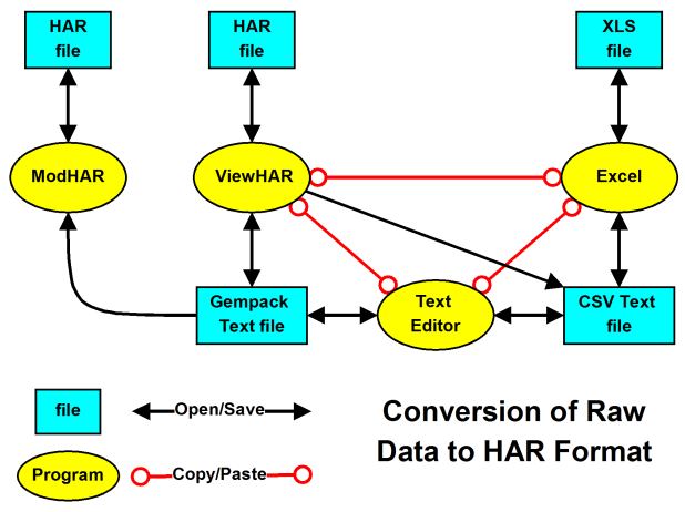
On a non-Windows operating system, the (rather old-fashioned) program MODHAR can be used to turn raw text data into a HAR file — as described in Chapter 54.
5.1.2 Processing raw data to create a HAR file that model can use [gpd4.3.2b]
Usually the raw data requires considerable processing or manipulation before it can be used by a CGE model. The best way to do this processing is via one or more data-manipulation TABLO programs. These TAB files contain COEFFICIENT, READ, FORMULA, and WRITE statements (but do not contain VARIABLE or EQUATION statements).
Figure 5.2 below shows a possible procedure. RAWDATA.HAR is created interactively in ViewHAR, by copying raw data from a spreadsheet. Then the sequence of programs, STEP1.TAB, STEP2.TAB and STEP3.TAB are used to turn the raw data into MODEL.HAR — which is formatted and arranged to be used by the actual CGE model (in MODEL.TAB). If the raw data was changed or updated, you would edit RAWDATA.HAR interactively in ViewHAR, then rerun the three programs STEP1 to STEP3.
Figure 5.2 Steps in processing raw data
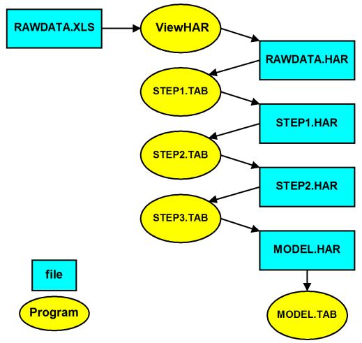
Clearly it would be risky or foolish to use ViewHAR to manually edit any of the files STEP1.HAR, STEP2.HAR or MODEL.HAR — any changes would be overwritten the next time you re-ran programs STEP1 to STEP3.
Using TABLO programs (rather than Excel) to process data offers three critical advantages:
- Most Excel programs work only with fixed dimensions for data arrays. That can be be a problem if you decide to, say, increase the number of sectors. By contrast, TABLO programs can be written to work with varying data dimensions.
- The TAB files provide a record of the operations that have been performed. By contrast, Excel operations leave no audit trail.
- If input data changes, it is easy to repeat processing by rerunning the TABLO programs. By contrast, it might be difficult or impossible to precisely repeat a complex sequence of Excel operations.
See section 38.3 for more about data-manipulation TABLO programs.
6 Constructing HAR files [gpd1.4]
Click here for detailed chapter contents
When you prepare the TABLO Input file for a model, you work out how much data is required (see section 4.2 above) and what it must represent. Then comes the (often difficult and time-consuming) task of assembling the actual data (numbers); we say nothing about this here. Once that has been done, you must create files containing these numbers which can be read by the GEMPACK programs. These files are usually GEMPACK Header Array files1.
Header Array files are binary files which contain one or more arrays containing data values. An individual array of data on a Header Array file is accessed by referring to the unique 4-character identifier known as a Header for that array of values. See chapter 5 for more details.
ViewHAR makes it fairly easy for you to create, view, or modify these files The use of ViewHAR to create Header Array files, and to modify data on them, is introduced in sections 6.1 and 6.2 below2.
The usual way of creating a Header Array data file is to start with data from another program or source in XLS or some text format.
For XLS source, blank arrays of the correct size are created in ViewHAR — then the numbers are pasted from Excel into these arrays. We illustrate this for Stylized Johansen in section 6.1 below.
Text source can often be edited into a form that ViewHAR can read directly -- the so-called GEMPACK text file format. Otherwise, it may be possible to read it into a spreadsheet to create XLS source.
Section 6.2 below contains examples which show how ViewHAR can be used to modify data on Header Array files.
When you construct a data base for a model, it is important to check that it is balanced. We give some examples in section 6.3 below.
GEMSIM and TABLO-generated programs can be used to write Header Array or text data files. We give a hands-on example and some details in section 38.3 below.
We provide a table in section 6.4 which summarises the different programs you can use to convert data files of one type (for example, a text data file) to another type (for example, a Header Array file).
There are many techniques used in preparing and modifying data. In this chapter we only scratch the surface. We recommend sources of further information in section 6.5.
6.1 Constructing the header array data file for Stylized Johansen [sjmkdat]
You have looked at the Header Array data file SJ.HAR for Stylized Johansen in section 3.4.3 above. In this section we take you through the steps to construct that file SJ.HAR. We recommend that you carry out these steps on your own computer.
As you have seen in section 4.2.1 above, we need three arrays of data for DVCOMIN, DVFACIN and DVHOUS; these are of size 2 x 2, 2 x 2 and 2 respectively. The matrices of data required are as shown in the data base in Table 3.1 of section 3.1.1. We assume that you have data in an Excel sheet (SJDAT.XLS in the examples folder), as shown in the table below.
Table 6.1 Excel sheet of data for SJ model
| Coefficient: | DVCOMIN | Header: | CINP |
| Dimensions: | SECT*SECT | Description: | Use of commodities by industries |
| s1 | s2 | ||
| s1 | 4 | 2 | |
| s2 | 2 | 6 | |
| Coefficient: | DVFACIN | Header: | FINP |
| Dimensions: | FAC*SECT | Description: | Inputs of primary factors |
| s1 | s2 | ||
| labor | 1 | 3 | |
| capital | 1 | 1 | |
| Coefficient: | DVHOUS | Header: | HCON |
| Dimensions: | SECT | Description: | Household use of commodities |
| s1 | 2 | ||
| s2 | 4 |
Step 1 — Create a new HAR file in ViewHAR
Open ViewHAR and open the file SJDAT.XLS in Excel (or similar program).
In ViewHAR there are two modes: the simplest is Read Only mode where you can look at a Header Array file and are not allowed to change it. To get to this mode, select from the File menu Use simplified, read-only menu.
The second mode is Editing mode where you are allowed to modify data in the Header Array file. To get to this mode, select from the File menu Use advanced, editing menu. You must be in Editing mode to carry out the operations described below.
From the File menu, select Create New File.
Step 2 — Create the needed sets
We can see from the Excel file that sizes of needed data arrays are given by the 2 sets SECT and FAC. The first step is to create ViewHAR headers for these 2 sets.
Use the command Sets | Create New Set to open the Create Set dialog for the set SECT. Type in
- the set name: SECT
- the set size: 2
- the description: Sectors
- the header: SEC
- the elements: S1 S2 (one per line)
Press the Check button to see if the data satisfies GEMPACK's rules. Press OK when you are done. You should see that the file now contains 1 header, "SEC".
Similarly use the Create Set dialog to make a header for the set FAC. Type in
- the set name: FAC
- the set size: 2
- the description: Primary factors
- the header: FAC
- the elements: Labour Capital (one per line)
For larger sets, it is easier to copy/paste the elements from Excel.
Now use File | Save as to save All headers in HAR format with the name MySJ.HAR.
Step 3 — Create the needed blank arrays
We can see from the Excel file that the needed data arrays are:
- DVCOMIN, dimensions SECT*SECT DVFACIN, dimensions FAC*SECT, and DVHOUS, dimension SECT
First use the Edit | Create new headercommand to make DVCOMIN. Fill in or choose the following options:
- the Header type: Real
- the header: CINP
- default value: 0
- the Coefficient name: DVCOMIN
- the description: Use of commodities by industries
- the no. of dimensions: 2
- Choose Sets: SECT in both drop down lists.
Press OK when you are done. You should see that the file now contains a new header, CINP. Examine the values of this header — they will be all zero, but at least you have an array of the right size with the right labels.
Leave this array (of zeros) in view in ViewHAR. Then, in Excel, select the 2x2 array of values3 for DVCOMIN, and Copy them to the clipboard.
Now go back to ViewHAR (still with the blank DVCOMIN array visible) and choose Import | Paste to screen from Clipboard. You should see the right numbers appear.
Now use File | Save to save your work4 so far.
Similarly, create and populate the DVFACIN and DVHOUS arrays.
Use Edit | Create new header to make DVFACIN by filling in or choosing: the Header type: Real; the header: FINP; the default value: 0; the Coefficient name: DVFACIN; the description: Inputs of primary factors; and the no. of dimensions: 2. For Choose Sets: select FAC in the first drop down list, and SECT in the second. Press OK when you are done.
Examine the values of the new FINP header — they will again be all zero. Then, in Excel, select the 2x2 array of values for DVFACIN, and Copy them to the clipboard. Then back in ViewHAR use Import | Paste to screen from Clipboard to bring the numbers into ViewHAR. And again File | Save .
For DVHOUS, similarly Edit | Create new header choose or fill in the Header type: Real; the header: HCON; the default value: 0; the Coefficient name: DVHOUS; the description: Household use of commodities; and the no. of dimensions: 1. For Choose Sets: select SECT in the drop down list. Press OK and view the new header HCON. Then, in Excel, select the 2 values for DVHOUS, and Copy them to the clipboard. Then back in ViewHAR use Import | Paste to screen from Clipboard to bring the numbers into ViewHAR. And yet again File | Save .
The task is complete !
6.1.0.1 Another way to attach set and element labelling information [sjmkdat2]
In the example above, we first created the sets, then used these to create blank labelled arrays. A more old-fashioned (but sometimes still useful) way is to first create blank un-labelled arrays, then create the sets, then attach sets to the arrays as row or column labels. You can do the latter with the menu item Edit | Apply/Change Set Labels . Use the Choose Dimension box in the bottom left-hand corner to select the first dimension. Then, with Choose Set drop-down list on the right-hand part of the form, select the right set. Then use the Choose Dimension box to select the second dimension, and the Choose Set drop-down list to select the right set for that. And so on, until all dimensions are labelled.
6.2 Editing the header array data file for Stylized Johansen [sjmoddat]
You can modify a number in ViewHAR by right-clicking that number (in the Data window) and typing in a new value.
To modify a whole array, it's usually easier to
- Use the command Export | Copy Screen to Clipboard
- Paste the array (with labels and totals) into a blank Excel sheet. Then modify the numbers as you wish. Make sure that plenty of decimal places are visible.
- Back in ViewHAR use Import | Paste to screen from Clipboard. You should see the new numbers appear.
Whether pasting numbers from Excel to ViewHAR, or from ViewHAR to Excel, you only get the number of decimal places that is visible in the source. Usually you need to increase the number of visible decimal places before you copy.
6.2.1 Other ViewHAR capabilities [gpd1.4.5.8]
ViewHAR offers many other capabilities. You can find more information in section 36.2, and complete details in the Help file supplied with ViewHAR.
6.3 Checking data is balanced [gpd1.4.7]
When you prepare the data file(s) for a model, you must be careful to check that all the different balancing conditions are satisfied.
For example, for Stylized Johansen, costs in each industry must equal the total demand for the corresponding commodity. In ORANI-G, which allows each industry to produce several commodities, there are two balancing conditions: costs in each industry must equal the value of all outputs from that industry; and output of each commodity (from several industries) must equal the total demand for that commodity.
The TAB file for a well-constructed model will contain code to check that such balance conditions hold, and even assertions (see section 25.3) that will stop the model running if they do not hold. Nonetheless, it is common (perhaps as part of a sequence of programs to produce a database) to write a self-contained TABLO Input file to read the data and carry out the calculations to check the balancing conditions. Such a TAB file will write the results of its calculations to a file you can look at to check that values are in balance.
When you are checking balance, you need to keep in mind that GEMPACK programs only produce about 6 figures of accuracy (see section 25.8).
6.3.1 SJCHK.TAB to check balance for Stylized Johansen [gpd1.4.7.1]
Supplied with GEMPACK is the file SJCHK.TAB which is used to check the balance of a data set for Stylized Johansen. View this file to see that the values of Coefficients DVCOM (value of output of each commodity) and DVCOSTS (costs in each industry) and the difference of these two (should be zero) are calculated and written to an output file. An Assertion statement (see section 25.3) is included so that the program will stop with an error if the difference is significant.
You will also see that a check is made to count the number of negative numbers in the data base (there should be none).
We encourage you to run SJCHK.TAB on SJ.HAR to check the balance.
If you prefer to use WinGEM, first make sure that both default directories point to the directory in which the Stylized Johansen files are located. First run TABLO on SJCHK.TAB and produce output for GEMSIM (for simplicity). Then run GEMSIM using Command file SJCHK.CMF. When GEMSIM has run, click on View Input/Output files and look at the values of DVCOM, DVCOSTS, and BALCHECK in the output file SJCHK.HAR. Also check that there are no negatives in the data base.
If you are working from the command prompt, change into the directory to which you copied the Stylized Johansen files. Then run TABLO on sjchk.tab to produce output for GEMSIM (for simplicity), ie, type:
TABLO -pgs sjchk
Then run GEMSIM taking inputs from the Command file sjchk.cmf, ie, type:
GEMSIM -cmf sjchk.cmf
When GEMSIM has run, look at the values of DVCOM, DVCOSTS, and BALCHECK in the output file sjchk.har, and also check for negative values.
6.3.2 SJCHK.TAB to check balance of updated data [gpd1.4.7.2]
Whenever you carry out a simulation, the updated data should satisfy the same balance checks as the original data — otherwise there is something wrong with the TAB file for your model.
It is easy to use SJCHK.TAB to check the balance of the updated data SJLB.UPD produced in the 10 percent labor increase simulation carried out via SJLB.CMF (see chapter 3). To do this, save the file SJCHK.CMF as SJLBCHK.CMF and alter the statement
file iodata = SJ.HAR ;
to read
file iodata = sjlb.upd ;
Then run GEMSIM taking inputs from Command file SJLBCHK.CMF. Look at the output file SJLBCHK.HAR produced and check that SJLB.UPD is still balanced.5
A more sophisticated, production-quality model should include such checking code in its main TAB file. That way, checking occurs every time the model runs — so alerting you early to potential problems.
6.3.3 GTAPVIEW for checking and summarising GTAP data [gpd1.4.7.3]
The standard GTAP TAB file referred to as GTAPVIEW provides a summary of any GTAP data set. We have provided GTPVEW61.TAB with the GEMPACK examples. You can see an example of the use of this TAB file in section 25.8.1.
The file GTPVEW61.TAB is an interesting example of a TAB file. For example, look at the set GDPEXPEND and how the values in Coefficient GDPEXP are built up via several Formulas. This shows a neat way of arranging summary data into headers on a Header Array file. You may be able to adapt some of these techniques in your own work.
6.3.4 Checking the balance of ORANIG data [gpd1.4.7.4]
See section 25.8.2 for details about this.
6.4 Which program to use in file conversion? [gpd1.4.8]
You need to convert between file formats
- at the start of the process of constructing a model database, when raw data in various formats need to be first stored in HAR files;
- after a simulation, when results in SL4 (and perhaps HAR) files need to be comunicated to other programs, such as Excel, Matlab, or MsWord.
ViewHAR can be used interactively to do many conversions; but if a process is to be automated, command-line programs (if available) are preferred — they can be run from batch (BAT) scripts.
Table 6.2 below shows which programs to use in converting files from one type to another. The table rows (source) and columns (destinations) are labelled with 3-letter abbreviations, as follows:
| HAR | GEMPACK Header array file |
| XLS | Excel Speadsheet file |
| CSV | text file as saved or read by Excel; may be comma-, tab- or space-delimited |
| SQL | text file in "database" format; one number per row; zeros not shown |
| TXT | GEMPACK text file: a special type of CSV, see chapter 38 |
| GDX | binary data file used by GAMS |
| SL4 | GEMPACK solution file |
Table 6.2 Programs to use in file conversion
| ↓In Out→ | HAR | XLS | CSV | SQL | TXT | GDX | |
| HAR | = | har2xls head2xls | head2csv seehar | har2csv | har2txt | har2gdx | |
| XLS/X | xls2head | = | Excel | - | Excel | - | |
| CSV | - | - | = | - | - | - | |
| SQL | csv2har | - | - | = | - | - | |
| TXT | modhar txt2har | ViewHAR | - | ViewHAR | = | ViewHAR | |
| GDX | gdx2har | ViewHAR | - | ViewHAR | ViewHAR | = | |
| SL4 | sltoht | ViewHAR | sltoht | ViewHAR | ViewHAR | ViewHAR |
In many cases alternative programs could be used; for example, ViewHAR can do most conversions. The table above shows the most appealing command-line program, if there is one — otherwise ViewHAR is shown. Note that from 2012 xls2head can read either XLS or XLSX files, but har2xls, head2xls and ViewHAR create only the older-format XLS files.
The programs gdx2har and har2gdx (see section 77.1) are command-line Windows-only programs distributed with GEMPACK. Slightly different versions are distributed with GAMS.
The programs har2csv, csv2har, har2txt, txt2har, har2xls, head2csv, head2xls and xls2head are command-line Windows-only programs. If they are not already included in your GEMPACK installation, you can download them from the GEMPACK website at http://www.copsmodels.com/gpmark9.htm. To obtain instructions for using, say, txt2har, you would simply type from the command line:
txt2har
In the table above "SQL" means, text files with lines like this:
"CitrusFruit","France","Germany","2005", 3974.2
meaning that, eg, 3974.2 tonnes of citrus was exported from France to Germany in 2005. Seehar's SQL option also offers a (fairly heavy-duty) way to turn HAR into SQL (see section 37.1.4).
For more about MODHAR, see chapter 54; for SEEHAR see chapter 37; and for SLTOHT see chapters 39 and 40.
To extract results from SL4 solution files, SLTOHT may be used to convert into one of two formats:
- a CSV text spreadsheet file which may be read by Excel — see chapter 40. A spreadsheet mapping file is used to select particular results.
- a HAR file — see chapter 39. A header mapping file is used to select particular results. The HAR file might be processed by a TABLO program or it might be converted to another format using one of the programs listed in table 6.2.
See also Running SLTOHT from the command line.
6.5 Further information [gpd1.4.9]
There are many techniques used in preparing and updating data files for models. This chapter is just a very brief introduction to the topic. Suggestions for finding out more are given below.
Aggregation: ViewHAR or, better, a command-line program AggHAR can be used to aggregate data. Both methods are described in the ViewHAR Help.
TABLO Input files: see example using mappings in section 11.9.
Disaggregation: can can be carried out using the (old-fashioned) command-line program DAGG downloadable from http://www.copsmodels.com/gpmark.htm. Alternatively, the newer command-line program DaggHAR (instructions in DaggHAR.doc) may be more convenient. In most cases, you will also need to write a TABLO program to do some of the job.
Periodic courses on the preparation of data for CGE models are listed at
http://www.copsmodels.com/pgemdata.htm
7 GEMPACK file types, names and suffixes [gpd1.5.8]
Click here for detailed chapter contents
GEMPACK programs use a number of different file types to communicate between themselves or to store results. Usually the file-name suffix (extension) indicates the file type.
7.0.1 Files with system-determined suffixes [gpd1.5.8.1]
Some types of files must be given system-determined suffixes. For example, GEMPACK requires that TABLO Input files have suffix .TAB. Below we list the most important type of files with system-determined suffixes (see also 3.14.1).
Table 7.1 File type with system-determined suffixes
| File type | Suffix | Type | See |
| TABLO Input file | .TAB | text | section 4.3 |
| TABLO Information file | .INF | text | section 9.1.6 |
| Solution file | .SL4 | binary | chapter 27 |
| Equations file | .EQ4 | binary | chapter 59 |
| GEMSIM Auxiliary Statement file | .GSS | binary | section 3.14.2 |
| GEMSIM Auxiliary Table file | .GST | binary | section 3.14.2 |
| TABLO-generated Auxiliary Statement file | .AXS | binary | section 3.14.2 |
| TABLO-generated Auxiliary Table file | .AXT | binary | section 3.14.2 |
| TABLO-generated program | .FOR | text | section 3.14.2 |
| Environment file | .EN4 | binary | section 23.2.5 |
| Model Information file | .MIN | text | section 21.4.1 |
| Solution Coefficients file | .SLC | binary | section 28.1 |
| Extrapolation Accuracy file | .XAC | text | section 3.12.3 |
Whenever a program asks you for the name of any of these files with system-determined suffixes, you should never include the suffix in your input (since the program will add the suffix automatically). For example, in a Command file put
Solution file = sjlb ; ! Correct
rather than
Solution file = sjlb.sl4 ; ! Incorrect
Similar to the .SLC Solution Coefficients file, are .UDC, .AVC, and .CVL files -- see sections 28.2 and 28.3.
7.0.2 Suffixes of other files [gpd1.5.8.2]
Even though GEMPACK does not force you to use specific suffixes for other files, there are several different types of files where it has become customary amongst experienced GEMPACK users to use certain suffixes. Examples are in the table below.
Table 7.2 Commonly used suffixes for other files
| File type | Usual Suffix(es) | Type | See |
| Header Array data file | .HAR | binary | chapter 5 |
| Text data file | .TXT | text | chapter 38 |
| Updated Header Array file | .UPD, .HAR | binary | section 3.9 |
| Command file | .CMF | text | chapter 20 |
| Stored-input file | .STI, .INP | text | section 48.3 |
| Spreadsheet Mapping file | .MAP | text | section 40.1 |
| Solution file in HAR form | .SOL | binary | section 39.1 |
In some cases there are considerable advantages from using these "usual" suffixes. For example,
- some Command file syntax is only available if you use suffix .CMF (see section 20.5).
- when you open a Header Array file with ViewHAR, by default it only shows you files with suffixes .HAR, .DAT, .UPD, .SUM, .SOL, .SLC, .SL4, .CVL, .UDC, .AVC, and .PRM.
- when you install GEMPACK, certain file suffixes are "associated" with GEMPACK programs. For example, .TAB and .CMF files are associated with TABmate — this means that in Explorer the TABmate icon is shown beside these files and you can double-click on them to open them in TABmate. Similarly .HAR and .UPD files are associated with ViewHAR, and .SL4 files are associated with ViewSOL.
Many of the GEMPACK programs suggest suffixes for output files they create. For example, SEEHAR often suggests suffix .SEE for its output files. We suggest that you go along with these suggestions unless you have good reasons to do otherwise.
7.0.3 Files — binary, header array or text? [gpd1.5.8.3]
There are two basic file types on all computers — text files (which are sometimes called ASCII files) and binary files. Text files are more portable — they can be viewed or printed using any text editor. Binary files are more compact and faster to process, but use one of a number of proprietary formats — so only special programs can read or create them. GEMPACK uses several files of each type, as indicated in tables 7.1 and 7.2.
Header Array (HAR) files (see chapter 6) are important binary files used often in GEMPACK to hold data for models. Although not recommended, you can also hold such data in text files: when used for this they must follow a standard format described in chapter 38.
7.0.4 Why so many files? [gpd1.5.8.4]
We have listed many of the important files, and discussed their roles, in section 3.14 above.
Some files are created to facilitate communication between different GEMPACK programs. [For example, GEMSIM Auxiliary files allow communication between TABLO and GEMSIM.]
Other files are created for users to look at or use. Some contain information which is important in reporting simulation results while others may allow experienced modellers to carry out tasks more efficiently. For example, when GEMSIM or a TABLO-generated program runs, it may produce various files listed below.
- The updated data (UPD) files provide information about the simulation and can be used as the starting point for other simulations (see section 3.9).
- The Equations (EQ4) file can be used as the starting point for Johansen simulations using SAGEM (see chapter 58).
- The Extrapolation Accuracy (XAC) file can be used to tell if the solution produced is sufficiently accurate for your purpose (see section 3.12.3). (If not, you may need to re-run it with more steps.)
- An Environment (EN4) file. Saving an Environment file makes it easy to run a different simulation with the same closure: you simply give the name of the Environment file instead of having to re-specify which of the variables are exogenous or endogenous. See section 23.2.5.
7.1 Allowed file and directory names [gpd1.5.9]
Both Windows1 and GEMPACK impose certain restrictions on file and directory names:
- File names are not case sensitive. So, for example, there is no distinction between the file names SJ.HAR and sj.har. Thus, if you create a new file called "sj.HAR" you will, in the process, delete any existing file called SJ.har or sj.HAR.
- GEMPACK programs never access or produce files whose names end with one or more spaces. For example, if you try to create a file called "xx.out " the trailing space will be omitted and the file "xx.out" will be created. Also the last character should not be a period (.).
- GEMPACK programs do not reliably support file names containing Chinese or other non-English characters. We apologise for this inconvenience.
- GEMPACK Windows programs (WinGEM, ViewHAR etc) do not reliably support file names containing "%" or "#" so we advise you to not to use these characters.
- You may not use characters \ / : * ? & < > or | in file names.
- We advise you not to use characters ; ! ( ) or = in file names.
- VERY long file and folder names should be avoided.
Directory names are restricted in the same way that file names are. Even if you are trying to create a file with a legal name, it may not be possible to create the file in a directory with an illegal name. For example, Chinese or Scandinavian characters in a directory name may cause problems.
Previous versions of GEMPACK and Fortran imposed tighter restrictions on file and directory names -- see section 5.9 of GPD-1. You might still be using a few older GEMPACK programs. To maintain compatibility with those:
- Stick to letters, digits, "-" and "_" (and avoid spaces) in your file and folder names.
Another virtue of the above rule is that is simpler to remember than the more complex rules above.
7.1.1 File names containing spaces [gpd1.5.9.4]
To specify a file name containing spaces in a Command (CMF) file, enclose the name inside double quotes:
solution file = "my sj" ;
See section 20.4.2 for details.
If you are running a program interactively, you must not add quotes "" when specifying file names containing spaces. Similarly you should not add quotes when specifying such file names in Stored-input (STI) files.
If you are specifying a Command file name, STI file name or LOG file name on the Command line (see section 48.5), enclose the name in double quotes "" if it contains a space as in, for example,
gemsim -cmf "c:\my sj\my sjlb.cmf"
7.1.2 Characters in stored-input files and command files [gpd1.5.9.5]
TAB characters and other control characters (ASCII characters 0-31 and 127) can cause problems in Stored-input files and Command files. TAB characters are replaced by a single space. Most control characters are replaced by a single space but will cause a warning message. The program will stop with an error message if it finds a Control-Z character before the end of the file if there is text after it, or if there are two or more in the file.
There is no testing for other characters (ASCII characters 128-255) but these would cause problems if used in file names — see section 7.1.
7.1.3 Files that could be deleted [cleanupfiles]
Section 3.14.8 list various filetypes that could be deleted to save space, or prior to backing up.
8 Overview of running TABLO and the TABLO language [gpd2.1]
Click here for detailed chapter contents
TABLO is the GEMPACK program which translates the algebraic specification of an economic model into a form which is suitable for carrying out simulations with the model. The output from TABLO can be either GSS/GST files used to run the GEMPACK program GEMSIM or alternatively, a Fortran program, referred to as a TABLO-generated program. When TABLO writes a TABLO-generated program, you must then compile and link (LTG) the program to create the EXE file of the TABLO-generated program. Either GEMSIM or the EXE file can be run to carry out simulations.
This chapter contains an introduction to running TABLO, to compiling and linking TABLO-generated programs, and to writing TABLO Input files.
Chapters 9 to 18 provide complete user documentation of the TABLO program and the TABLO language. TABLO is the means by which economic models are implemented within GEMPACK, as described in the introductory chapters 3 to 7 (which you should read first).
Chapter 9 provides some of the fine print about running TABLO, including how it linearizes levels equations and about its Condensation stage.
Chapter 10 is a full description of the syntax required in TABLO Input files while chapter 11 contains a comprehensive description of the semantics (and a few points about the syntax which may not be clear from chapter 10) for the current version of TABLO.
Chapter 12 describes the TABLO statements for post-simulation processing; chapter 13 builds on this to shows how ranked sets can be used to present tables of winning and losing sectors in a simulation.
Chapter 15 provides some assistance with the important task of verifying that your model is actually carrying out the calculations you intend. Chapter 16 provides some details about intertemporal (that is, dynamic) modelling in GEMPACK. In chapter 17 we give examples of ways in which the TABLO language can be used to express relationships which at first sight are difficult to capture within the syntax and semantics of TABLO Input files.
Chapter 18 gives rules for linearizing levels equations, and indicates how the linearized equations are shown on the Information file.
We expect that chapters 9 to 18 will be used mainly as a reference document (rather than being read through in order). Use the Index to help find the relevant part whenever you need more information about TABLO.
Chapters 19 to 35 describe carrying out simulations on economic models after they have been implemented using TABLO.
8.1 Running TABLO on an existing model [gpd2.1.1]
- Running TABLO from WinGEM is described in sections 3.5.2 and 3.5.3.
- See the examples in sections 43.3 and 43.4 of running TABLO for the models Stylized Johansen (SJ) and Miniature Orani (MO).
- See the examples in sections 43.5 to 43.8 where TABLO is run with a Stored-input file in order to condense the models GTAP and ORANIG.
Each of these examples assumes that you wish to run an existing model, or modify slightly an existing model.
You will find that TABmate (see section 8.4.1 below and section 36.4) provides an excellent interface for working with TABLO Input files, especially for identifying and eliminating syntax and semantic errors.
8.1.1 Example models ORANIG01 and GTAP61 [gpd2.1.1.1]
In chapter 3 the Stylized Johansen model SJ.TAB was used as the main example model. In following chapters the main example models are
(1) the ORANI-G model (May 2001) in the TABLO Input file ORANIG01.TAB written by Mark Horridge and colleagues from the Centre of Policy Studies, and
(2) the GTAP model Version 6.1 (August 2001) in the TABLO Input file GTAP61.TAB written by Tom Hertel and colleagues from the Center for Global Trade Analysis at Purdue University (see Hertel (1997) and McDougall (2002)).
The files for these models are amongst the Examples supplied with GEMPACK (see sections 60.5.1 and 60.7.1).
Running the ORANIG01 Model
View the ORANIG01 model in TABmate by opening ORANIG01.TAB from the GEMPACK Examples directory (usually C:\GP\EXAMPLES).
To run TABLO on the TABLO Input file ORANIG01.TAB, you should use the Stored-input file which carries out condensation.
(1) If you have a Source-code version of GEMPACK use the file OG01TG.STI to write a TABLO-generated program. At the Command prompt, the commands to use are
tablo -sti og01tg.sti            (creates TG-program ORANIG01.FOR).
ltg oranig01                     (compiles and links to produce ORANIG01.EXE).
Or you could click the TABLO STI button in TABmate (selecting og01tg.sti) to run both commands above.
(2) If you have the Executable-Image version of GEMPACK use the file OG01GS.STI. At the Command prompt, the command to use is
tablo -sti og01gs.sti (produces output for GEMSIM)
Or you could click the TABLO STI button in TABmate (selecting og01gs.sti) to run the command above.
(3) If you are working in WinGEM, select the TABLO option Run from STI file and then select the STI file OG01GS.STI or OG01TG.STI and then click on the Run button.
Running the GTAP61 Model
Similarly you can view the GTAP61 model by opening the file GTAP61.TAB from the GEMPACK Examples subdirectory in your text editor. This model also needs a condensation STI file to run successfully. The Stored-input file called GTAP61TG.STI writes a TABLO-generated program and GTAP61GS.STI writes auxiliary files for GEMSIM.
(1) If you have a Source-code version of GEMPACK use the file GTAP61TG.STI. At the Command prompt, the commands to use are
tablo -sti gtap61tg.sti   (creates TG-program GTAP61.FOR)
ltg gtap61   (compiles and links to produce GTAP61.EXE).
Or you could click the TABLO STI button in TABmate (selecting gtap61tg.sti) to run both commands above.
(2) If you have the Executable-Image version of GEMPACK use the file GTAP61GS.STI. At the Command prompt, the command to use is
tablo -sti gtap61gs.sti (produces output for GEMSIM)
Or you could click the TABLO STI button in TABmate (selecting gtap61gs.sti) to run the command above.
(3) If you are working in WinGEM, select the TABLO option Run from STI file and then select the STI file GTAP61GS.STI or GTAP61TG.STI and then click on the Run button.
Syntax and semantic examples from the TABLO Input files ORANIG01.TAB and GTAP61.TAB are used in throughout this chapter so that you can check a complete example of the relevant TABLO statements in a working model.
8.1.2 TAB file and WFP/PGS on command line [gpd5.10.1.2]
If you do not want to do any condensation actions not included in the TAB file, and you do not want to specify any options other than PGS or WFP at the Code stage, you can include the name of the TABLO Input file on the command line when you run TABLO. TABLO then runs in batch mode and does not expect any other input. If there are condensation actions in the TAB file, running with -pgs or -wfp will do those condensation actions (but give no opportunity for other condensation actions) and then go to Code stage.
- You specify the name of the TABLO Input file on the command line - don't include the suffix .TAB.
- You can specify PGS by putting -pgs on the command line.
- You can specify WFP by putting -wfp on the command line.
Examples
1: To run TABLO to process SJ.TAB
tablo sj
This will produce either a TABLO-generated program or output for GEMSIM, depending on which is the default action for the TABLO.EXE which is running. [The default is TABLO-generated program if TABLO.EXE is from a Source-code Version of GEMPACK or is GEMSIM if TABLO.EXE is from an Executable-Image Version of GEMPACK.]
2: To run TABLO to process SJ.TAB and produce output for GEMSIM
tablo -pgs sj
3: To run TABLO to process SJ.TAB and produce output for GEMSIM and send all output to file SJGS.LOG
tablo -pgs sj -log sjgs.log
4: To run TABLO to process SJ.TAB and produce the TABLO-generated program SJ.FOR
tablo -wfp sj
or
tablo sj -wfp
the order is not important.
If you specify the TABLO Input file on the command line1, it is the same as running TABLO interactively and hitting carriage-return for every response (except the TAB file and WFP/PGS choices).
8.1.3 Running TABLO from TABmate with no STI file [tablocode]
Similar to the above, the TABLO Code button in TABmate runs TABLO without a STI file. The Options...Code and Other menu item is used to control whether TABLO produces a Fortran program or GEMSIM output.
8.1.4 Preliminary pass to count statements [gpd2.1.1.2]
TABLO carries out a preliminary pass of the TABLO Input file. On this pass, it just counts the numbers of the different types of statements and allocates memory for the checking which follows on the second pass.
If a line of your TABLO Input file is too long (see section 11.1.2), this error is pointed out on the preliminary pass. In that case, TABLO does no other checking. You must fix this long line and then run TABLO again. You may find that there are errors above this position in the TAB file, since TABLO has not really checked anything except line length on the preliminary pass.
8.2 Compiling and linking TABLO-generated programs [gpd2.1.2]
"Compiling and linking" a TABLO-generated program refers to what has been called Step 1(b) in sections 3.5.2 and 3.6.1.
If you are working at the command prompt, the command LTG as in
LTG <program-name> (for example, ltg oranig01 or ltg gtap61)
will compile and link a TABLO-generated program.
If you are using WinGEM, you can compile and link via menu item Compile & Link... under WinGEM's Simulation menu.
Within TABmate, when either of the TABLO Code or TABLO STI buttons is used to produce a Fortran program, LTG may be run automatically (or you may be prompted — see the Options...Code and Other menu item.
The input to the compile and link process is the TABLO-generated program (for example, ORANIG01.FOR). The output is an EXE file for the TABLO-generated program (for example, ORANIG01.EXE). You run the EXE file to carry out simulations with the model.
8.3 Writing a TABLO input file for a new model [gpd2.1.4]
If you wish to develop a TAB file for your own model without relying on an existing model, how do you go about it? Chapter 4 describes how to build a new model using Stylized Johansen as a simple example. To summarise, the steps are as follows.
Write down your equations in ordinary algebra. Choose whether to write a linearized, mixed or levels model. You may need to linearize your equations by hand (see section 18.2).
Compile a list of variables used in these equations.
Compile a list of data needed for the equations (levels values, parameters, other coefficients).
Work out what sets are involved for the equations, variables and data.
Construct your TAB file in TABmate (see section 8.4.1 below) and keep checking the syntax (clicking the "TABLO check" button) until you have removed all syntax errors. Section 4.7.1 contains a hands-on example showing how to correct errors in TABLO Input files. Consult chapters 10 and 11 for the TABLO syntax needed to write your TABLO statements. Use other models as extended examples of how to write TABLO code.
If your model is large, you may need to condense it — see section 8.5 below.
You can run your model within WinGEM or at the Command prompt.The simulation process is described in chapter 3 and in more detail in chapters 19 to 35.
8.4 Modern ways of writing TABLO input files (on a PC) [gpd2.1.5]
Although you can create TAB files with any text editor (such as emacs, NotePad or vi), we suggest that you use GEMPACK's TABMate text editor.
8.4.1 Using TABmate [gpd2.1.5.1]
Unless you have a firm preference for another text editor, we recommend that you use the TABmate editor because it has many in-built functions to assist you including the following.
- Coloured highlighting of TABLO syntax, and of Command file syntax.
- Easy TABLO syntax checking allowing you to correct errors in the TAB file.
- A powerful Gloss feature which displays all parts of the TABLO code where a chosen variable or coefficient is used (see section 4.3.2 and section 46.1).
- You can have multiple files open and cut-and-paste between them in the usual Windows way.
More details about TABmate can be found in section 36.4.
8.4.2 Using TABmate to find a closure and suggest substitutions [autoclosure]
TABmate's Tools...Closure command helps you to find a standard closure for your GE model. It can also be used to find logical errors in your model, to suggest condensation actions, or to help construct a STI file. The results of the closure analysis are contained in a text report file suffixed CLO.
TABmate starts from the premise that there must be the same number of endogenous variables as equations in your model. By extension, we can usefully imagine that each equation explains a particular variable. Variables not explained by any equation are deemed to be exogenous in the standard closure.
In order for TABmate to know which variable is explained by a given equation, the modeller must follow a naming convention for equations. The convention is that the equation which explains variable "p1", say, is named "E_p1" (prefix E_). If you do not follow this convention, the Closure command will be no use to you, although the rest of TABmate will work normally.
Use the TABmate menu command Tools...Help on Tools to find out more about the Tools...Closure command.
8.4.3 Using TABmate to create a CMF file [autocmf]
TABmate's Tools...View/Create CMF will create a template CMF file for your model — you only need to add in the closure, shocks and actual filenames.
8.4.4 Using TABmate to reformat your code [beautyparlour]
TABLO is not case-sensitive: it will not complain if your TAB file refers to the same variable as "x1lab", "X1LAB" and "x1Lab". However, consistency is desirable, and can be enforced using TABmate's Tools...Beauty Parlour command. You can choose for, say, variables, to be rendered consistently in lower-case, or with the capitalization used when they first appeared in the TAB file.
8.4.5 Using ViewHAR to write TABLO code for data manipulation [gpd2.1.5.2]
If you have a Header Array data file containing set and element labelling (see section 5.0.3) and Coefficient names, ViewHAR can be used to write some of the TABLO code. To test this, run ViewHAR and open the file SJ.HAR from the GEMPACK Examples subdirectory. Select Export | Create TABLO Code from the main ViewHAR Menu. This will write some text to the Clipboard. In TABmate, create a new blank TAB file, and paste in text from the Clipboard. The following text will be created.
Example of TABLO code written by ViewHAR
Set SECT # description # (s1, s2);
Set FAC # description # (labor, capital);

Coefficient
(All,s,SECT)(All,a,SECT) DVCOMIN(s,a)
 # Intermediate inputs of commodities to industries - dollar values #;
(All,f,FAC)(All,s,SECT) DVFACIN(f,s)
 # Intermediate inputs of primary factors - dollar values #;
(All,s,SECT) DVHOUS(s) # Household use of commodities - dollar values #;.
Read
 DVCOMIN from file InFile header "CINP";
 DVFACIN from file InFile header "FINP";
 DVHOUS from file InFile header "HCON";

Update
(All,s,SECT)(All,a,SECT) DVCOMIN(s,a) = 0.0;
(All,f,FAC)(All,s,SECT) DVFACIN(f,s) = 0.0;
(All,s,SECT) DVHOUS(s) = 0.0;

Formula
(All,s,SECT)(All,a,SECT) DVCOMIN(s,a) = 0.0;
(All,f,FAC)(All,s,SECT) DVFACIN(f,s) = 0.0;
(All,s,SECT) DVHOUS(s) = 0.0;

Write
 DVCOMIN to file OutFile header "CINP" longname
 "Intermediate inputs of commodities to industries - dollar values";
 DVFACIN to file OutFile header "FINP" longname
 "Intermediate inputs of primary factors - dollar values";
 DVHOUS to file OutFile header "HCON" longname
 "Household use of commodities - dollar values";
ViewHAR has done all the dull part of code writing, and you can quickly edit the code by writing in appropriate filenames, formulas, updates etc to suit your model. This is very useful if you want to write a data manipulation TABLO Input file.
8.5 Condensing a large model [gpd2.1.6]
If your model is either too large to run on your computer, or too slow, you should consider condensation. See section 14.1 for an introduction to condensation, sections 14.1.2 and 14.1.4 for examples of condensation, and section 14.1.10 for further details. Basically you need to consider:
- Are there variables you can "omit", that is, variables that in this set of simulations will be exogenous and not shocked?
- Which are the endogenous variables with the largest number of components? These are candidates for substituting out or backsolving.
- To substitute or backsolve a variable, you need to identify a single equation which explains or determines that variable and is of the same dimensions.
TABmate's Tools...Closure command (see section 8.4.2) is extremely useful in suggesting condensation possibilities. Also very useful is the Condensation Information file: see section 14.1.16.
Recent versions of GEMPACK allow you to specify condensation actions within the TAB files via OMIT, SUBSTITUTE and BACKSOLVE statements: see section 10.16. That is the recommended approach. TABmate's Tools...Closure command will produce condensation commands that you can paste into your TAB file.
8.5.1 Condensation in STI file: a legacy technique [oldsticond]
The older method was to specify condensation actions in a STI or Stored-input file. As mentioned above, nowadays you should instead place OMIT, SUBSTITUTE and BACKSOLVE statements within the TAB file. TABmate's Tools...Create in-TAB condensation from STI command will convert condensation commands from an older STI file into this modern form.
If you still need to work with the old STI file method, the examples in section 14.1.2 show an older way to create a STI file for condensation, suitable for small models: you could run TABLO interactively to carry out condensation and to create a Stored-input file which can be re-used to carry out this condensation.
TABmate's TABLO STI button can create a default STI file — which you could add to. The Tools...Closure command will produce condensation commands that you can paste into the STI file.
Using a basic STI file as a starting point, you can easily add, using your text editor, other variables to omit, substitute or backsolve. When this Stored-input file is complete, run TABLO with this Stored-input file, and continue in the usual way, either compiling, linking and running the TABLO-generated program, or running GEMSIM.
Example - Stored-input files for ORANIG
Use TABmate to look at the Condensation file for ORANIG01.TAB. There are two versions: OG01GS.STI which creates output for the GEMPACK program GEMSIM (using the pgs option), and OG01TG.STI which creates the TABLO-generated program ORANIG01.FOR and its Auxiliary files ORANIG01.AXS and ORANIG01.AXT (using the wfp option).
9 Additional information about running TABLO [gpd2.2]
Click here for detailed chapter contents
Most of the information about running TABLO is given in chapters 3 and 4. This chapter (which you could skip during a first reading) provides some additional, advanced information relating to:
- the TABLO Options screens (section 9.1),
- how TABLO linearizes levels equations (section 9.2),
- reporting Newton error terms in models with levels equations (section 9.3).
9.1 TABLO options [gpd2.2.1]
This section gives details about Options that are available at the TABLO Check stage. Chapter 50 gives details about options available at the TABLO Code stage.
The TABLO program is divided into three distinct stages: CHECK, CONDENSE and CODE.
- In the CHECK stage, TABLO analyses the information on the TABLO Input file and points out any syntax errors (where the format expected by TABLO has not been followed) or semantic errors (where different parts of the input are not consistent with one another). Errors are output briefly to the screen and also to an Information file (usually with suffix .INF). Errors can be found by searching the Information file for %% which precedes each error message. (See section 9.1.6 below for more details.)
- The CONDENSE stage is optional. Details of condensation are given in section 14.1 and in section 14.1.10 below.
- The CODE stage either writes output for GEMSIM or writes the TABLO-generated program which corresponds to the TABLO Input file.
On starting TABLO, you make selections from the TABLO Options menu shown below. Standard Basic Options LOG, STI, SIF, ASI, BAT, BPR at the top of the screen are described in chapter 48.
You can choose which stages you carry out using the First Stage options (F1, F2, F3) and the Last Stage options (L1, L2, L3). The default choices for these options are F1 for the First Stage and L3 for the Last Stage. These mean that TABLO starts with the CHECK stage, then, if no errors are encountered during the CHECK, carries out CONDENSE (if requested), and then goes on to the CODE stage.
The option of carrying out some stages only is rarely used (except by GEMPACK developers doing debugging). There is more about it in section 64.1.
                  TABLO OPTIONS
             ( --> indicates those in effect )

     BAT Run in batch              STI Take inputs from a Stored-input file
     BPR Brief prompts             SIF Store inputs on a file
     LOG Output to log file        ASI Add to incomplete Stored-input file

     First Stage                   Last Stage
     -----------                   ----------
 --> F1 CHECK                      L1 CHECK
     F2 CONDENSATION               L2 CONDENSATION
     F3 CODE GENERATION        --> L3 CODE GENERATION

     RMS Require maximum set sizes to be specified
     NTX Dont store TAB file on Auxiliary file
     ICT Ignore Condensation statements on TAB file
     ASB All Substitutions treated as Backsolves
     NWT Add Newton-correction terms to levels equations
     ACD Always use Change Differentiation of levels equations
     SCO Specialized Check Options menu

 Select an option   :  <opt>      Deselect an option      : -<opt>
 Help for an option : ?<opt>      Help on all options     : ??
 Redisplay options  : /           Finish option selection:Carriage return
Your selection >

                    Main TABLO Options Menu
Option ACD is discussed in section 9.2.4 below. It affects the way TABLO linearizes any levels equations which, in turn, can affect the numerical properties of multi-step calculations.
Option RMS (Require Maximum Set Sizes) affects the CHECK stage of TABLO. When this option is selected the statement
SET REG # Regions # READ ELEMENTS FROM FILE GTAPSETS Header "H1";
would produce a semantic error. See section 11.7.2 for details.
Option NWT could be used with Newton's method to solve equations (see section 26.6). It causes TABLO to add the $del_newton term to all levels equations.
Option NTX is described in section 9.1.1 below. Option SCO leads to other options as described in section 9.1.3 below. Options ICT and ASB, which relate to the Condensation stage of TABLO (see section 14.1.10 below), are described in sections 14.1.15 and 14.1.13 respectively below.
9.1.1 TABLO input file written on the auxiliary files [gpd2.2.1.1]
The TABLO Input file for your model is written to the Auxiliary Table file (.AXT for a TABLO-generated program, .GST for GEMSIM) by default. These files are HAR files — but would only be meaningful to the GEMPACK developers. You can use the program TEXTBI (see chapter 70) to recover the Stored-input file from the Auxiliary Table file.
If, for reasons of confidentiality, you do not wish to send out your TABLO Input file on the Auxiliary files, you can turn off this default. At the first option screen in TABLO or at the top of your condensation Stored-input file, select the option
NTX Don't store the TAB file on Auxiliary file
then continue as usual with the TABLO input.
9.1.2 TABLO file and TABLO STI file stored on solution file [gpd2.2.1.2]
When the TABLO Input file is stored on the Auxiliary Table (.AXT or .GST) file (see section 9.1.1 above), this TABLO Input file is transferred from the Auxiliary Table file to the Solution file when you carry out a simulation using GEMSIM or a TABLO-generated program. This means that you can use the program TEXTBI (see chapter 70) to recover that TABLO Input file from the Solution file. This may assist in understanding simulation results.
Similarly, if you use a Stored-input file to run TABLO, this Stored-input file is transferred to the Auxiliary Table file produced by TABLO (unless TABLO option NTX is selected)
This Stored-input file is also transferred to the Solution file when you run a simulation using GEMSIM or a TABLO-generated program. You can use TEXTBI (see chapter 70) to recover the Stored-input file from the Solution file or from the Auxiliary Table file. [Strictly speaking, the Stored-input file put on the Auxiliary Table file is the one used for the CODE stage of TABLO. If you stopped and restarted TABLO (see section 64.1) condensation actions may not be on the Stored-input file put on the Auxiliary Table or Solution file.]
Note that the Stored-input file is only stored on the Auxiliary Table file if you use the STI option (see section 48.3) in TABLO by inputting
tablo.sti.sti-file-name
or the -STI option on the command line (see section 48.5) as in
tablo -sti sti-file-name
It does not happen if you use input redirection as in
tablo < sti-file-name ! NOT recommended
since in this case TABLO is not aware that you are using a Stored-input file.
This means that it is usually possible to recover the TABLO file and any condensation actions from any Solution file.
Since the original data is stored on the SLC file (see section 28.1), this means that you can recover everything about a simulation from the Solution and SLC files.
9.1.3 Specialised check options [gpd2.2.1.3]
Choosing SCO gives access to the Specialised Check Options menu given below. However these options are rarely used so TABLO uses the default values for these unless you actively choose SCO and one or more of the Specialised Check options. You can find out more about these options from this menu. [For example, type ?SM5 to find out about option SM5.]
                Specialised Check Options
              ( --> indicates those in effect )

       Semantic Check Options
       ----------------------
       SM2 Allow duplicate names
       SM3 Omit coefficient initialisation check
       SM4 Omit checking for warnings
       SM5 Do not display individual warnings

       Information File Options
       ------------------------
       IN1 Has the same name as the TABLO Input file
       IN2 Only show lines containing errors
       IN3 Omit the model summary in CHECK stage

Select an option   :  <opt>  Deselect an option      : -<opt>
Help for an option : ?<opt>  Help on all options     : ??
Redisplay options  : /       Return to TABLO Options : Carriage return
Your selection >

                  Specialised Check Options Menu
9.1.4 Doing condensation or going to code generation [gpd2.2.1.4]
After the CHECK stage is complete, if no syntax or semantic errors have been found, you are given the choice below:
  Do you want to see a SUMMARY of the model        [s], or
              perform CONDENSATION                 [c], or
              proceed to AUTOMATIC CODE GENERATION [a], or
              EXIT from TABLO                      [e] :

   (Enter a carriage return to proceed directly
      to AUTOMATIC CODE GENERATION)
If you select [a] (or if you type a carriage return), you will skip condensation and go directly to the Code stage of TABLO.
If you select [c], the following choice is presented. See section 14.1 and section 14.1.10 below for a description of Condensation.
 --> Starting CONDENSATION

  Do you want to SUBSTITUTE a variable             [s], or
      substitute a variable and BACKSOLVE for it   [b], or
                 OMIT one or more variables        [o], or
                 ABSORB one or more variables      [a], or
                 DISPLAY the model's status        [d], or
                 EXIT from CONDENSATION            [e] :
If you select [e] at either of the last two choices, the TABLO Record file (.TBR) and the Table file (.TBT) [see section 64.1] are written and the program TABLO ends.
9.1.5 TABLO code options [gpd2.2.1.5]
When you proceed to Automatic Code Generation, a Code Options Menu is presented. The main choice here is whether to produce output for GEMSIM (option PGS) or to write a TABLO-generated program (option WFP). Because the effect of the other options is intimately bound up with the way GEMSIM or the resulting TABLO-generated program will run, we postpone a discussion of these options until chapter 50.
9.1.6 Identifying and correcting syntax and semantic errors [gpd2.2.1.6]
If TABLO finds syntax or semantic errors during the CHECK stage, it reports them to the terminal and also, more usefully, to the Information (.INF) file.
To identify these errors, look at the Information file (via a text editor, or print it out). Syntax and semantic errors are marked by two percent signs %%, so you can search for them in an editor. The Information file usually shows the whole TABLO Input file (with line numbers added); lines with errors are repeated and a brief explanation is given of the reason for each error. (Also a question mark '?' in the line below the line with an error points to the part of the line where the error seems to be.)
Usually the change needed to correct the error will be clear from the explanation given. If not, you may need to consult the relevant parts of chapter 10 (for syntax errors) or chapter 11 (for semantic errors).
One syntax or semantic error may produce many more. If, for example, you incorrectly declare a COEFFICIENT A6, then every reference to A6 will produce a semantic problem ("Unknown coefficient"). In these cases, fixing the first error will remove all consequential errors.
TABmate (see section 8.4.1 above and section 36.4) provides an excellent interface for working with TABLO Input files, especially for identifying and eliminating syntax and semantic errors.
9.2 TABLO linearizes levels equations automatically [gpd2.2.2]
This section is only relevant for TABLO Input files which contain explicit levels EQUATIONs or explicit levels VARIABLEs.1 During the CHECK stage, when TABLO processes a TABLO Input file containing levels EQUATIONs and levels VARIABLEs, it converts the file to a linearized file; we refer to this as the associated linearized TABLO Input file. Although you may not see this associated linearized file (since the conversion is done internally by TABLO), you should be aware of some of its features.
The most important feature of this conversion is that, for each levels VARIABLE, say X, in your original TABLO Input file, there is an associated linear VARIABLE whose name is usually that of the original levels variable with "p_" added at the start.2 Also, for each levels VARIABLE in the original TABLO Input file, a COEFFICIENT with the same name as the levels VARIABLE is declared in the associated linearized TABLO Input file.
Other features of this conversion will be explained in sections 9.2.1 to 9.2.4 below.
It is important to realise that the rest of TABLO (the last part of the CHECK and all of the CONDENSE and CODE stages) proceeds
as if the associated linearized TABLO Input
file were the actual TABLO Input
file.
This means that during CHECK and CONDENSE, warnings and error messages may refer to statements in this associated linearized file rather than in your original TABLO Input file.
During the CHECK stage, TABLO normally echoes the original TABLO Input file to the Information file (and flags any errors or warnings there). When there are levels EQUATIONs in the original file, in the Information file which TABLO writes to describe this model, each levels EQUATION is followed by its associated linearized EQUATION. So, if you wish to see the associated linearized EQUATIONs you can do so by looking at the CHECK part of the Information file. In section 18.3 we show part of the Information file obtained from processing the TABLO Input file SJ.TAB for the mixed version of Stylized Johansen. You can look there to see the linearized EQUATIONs associated with some of the levels EQUATIONs from this TABLO Input file, which is shown in full in section 4.3.3.
9.2.1 Change or percentage-change associated linear variables [gpd2.2.2.1]
When you declare a levels VARIABLE in your TABLO Input file, you must also decide which form of associated linear VARIABLE you wish to go in the associated linearized TABLO Input file. If you want it to be the corresponding percentage change, you don't need to take special action since this is usually the default. If however you wish it to be the corresponding change, you must notify TABLO of this by including the qualifier (CHANGE) in your VARIABLE statement. For example, the statement
VARIABLE (LEVELS,CHANGE) BT # Balance of Trade # ;
in a TABLO Input file will give rise to a CHANGE variable c_BT in the associated linearized TABLO Input file.
As explained in section 4.3.5, there are some circumstances when a change linear variable is preferable to the percentage-change alternative. When you declare a levels VARIABLE we suggest the following guidelines.
- For a levels variable which is always positive (or always negative), direct TABLO to work with the associated percentage change as a linear VARIABLE in the associated linearized TABLO Input file.
- For a levels variable which may be positive, zero or negative, direct TABLO to work with the associated change as a linear VARIABLE in the associated linearized TABLO Input file. This can be achieved by declaring the levels VARIABLE via a VARIABLE(CHANGE) statement, as in, for example,
VARIABLE (LEVELS,CHANGE) BT # balance of trade # ;
9.2.2 How levels variable statements are converted [gpd2.2.2.2]
When you declare a levels VARIABLE or write down a levels EQUATION in a TABLO Input file, these give rise to associated statements in the associated linearized TABLO Input file created automatically by TABLO. After that, TABLO's processing proceeds as if you had actually written these associated statements rather than the levels statements actually written. We look at the different possibilities below.
Declaration of a Levels VARIABLE
Each declaration of a levels VARIABLE is automatically converted to three statements in the associated linearized TABLO Input file.3 These are
(1): the declaration of a COEFFICIENT(NON_PARAMETER) with the same name as the levels VARIABLE;
(2): the declaration of the associated linear VARIABLE if there is no LINEAR_VAR= qualifier. If there is a LINEAR_NAME= qualifier, that determines the name of this associated linear variable (see a few lines below). Otherwise the name of the associated linear variable has "p_" or "c_" added at the start depending on whether the corresponding percentage-change or change has been indicated by a qualifier PERCENT_CHANGE or CHANGE , or by the default statement currently in force if neither of these qualifiers is present;
(3): an UPDATE statement saying how the COEFFICIENT in (1) is to be updated during a multi-step simulation.
Example 1 The statement
VARIABLE (LEVELS,PERCENT_CHANGE) (all,c,COM) X(c) #label# ;
is converted to the 3 statements.
COEFFICIENT (NON_PARAMETER) (all,c,COM) X(c) ;
VARIABLE (LINEAR,PERCENT_CHANGE) (all,c,COM) p_X(c) #label# ;
UPDATE  (all,c,COM)  X(c) = p_X(c) ;
Example 2 The statement
VARIABLE (LEVELS,CHANGE) (all,i,IND) Y(i) #label# ;
is converted to the 3 statements
COEFFICIENT (NON_PARAMETER) (all,i,IND) Y(i) ;
VARIABLE (LINEAR,CHANGE) (all,i,IND) c_Y(i) #label# ;
UPDATE (CHANGE)   (all,i,IND)  Y(i) = c_Y(i) ;
Two Variable statement qualifiers LINEAR_NAME= and LINEAR_VAR= (see section 10.4) can alter the way in which a Levels Variable statement is converted.
Specifying the name of the linear variable (LINEAR_NAME)
You can use the qualifier LINEAR_NAME= if you want to specify the name of the associated linear variable (rather than letting TABLO determine the name by adding "p_" or "c_" to the front of the name of the Levels variable as described above).
For example
Variable(Levels, Linear_Name=xpc) (All,c,COM) X(c) ;
tells TABLO to use the name xpc (rather than p_X) for the linear variable associated with levels variable X. This statement is equivalent to the following three statements:
Coefficient (Non_parameter) (all,c,COM) X(c) ;
Variable (Linear,Percent_change) (all,c,COM) xpc(c);
Update  (all,c,COM)  X(c) = xpc(c) ;
Using a linear variable declared earlier (LINEAR_VAR)
You can use the qualifier LINEAR_VAR= if you want to indicate that the associated linear variable has been declared earlier in the TAB file. In this case TABLO adds the Coefficient and Update statements as indicated earlier but does not add a new Linear Variable. Instead TABLO associates the already declared Linear variable with this new Levels variable.
For example
Variable(Levels, Linear_Var=x) (All,c,COM) X_L(c) ;
tells TABLO that the linear variable to be associated with the levels variable X_L is the Linear Variable x declared earlier in the TAB file. This statement is equivalent to the following two statements:
COEFFICIENT (NON_PARAMETER) (all,c,COM) X_L(c) ;
UPDATE  (all,c,COM)  X_L(c) = x(c) ;
Use of the qualifier LINEAR_VAR= can reduce the proliferation of Variables and Equations when you add one or more Levels Variables at the bottom of a TAB file in which most equations are linearized ones.
For example, in ORANI-G there is a linear variable p0(c,s) giving the percentage change in the basic price of commodity c from source s (domestic or imported). Suppose that you need to add a Levels Equation involving this price. Then you need to add a levels version of this variable. Instead of using the qualifier LINEAR_VAR= you could add the following statements the end of the TAB file.
Variable(Levels) (All,c,COM)(All,s,SOURCE) P0_L(c,s) ;
Equation (Linear) E_p_P0_L  (All,c,COM)(All,s,SOURCE) p_P0_L(c,s) = p0(c,s) ;
Here the equation is needed to connect the two linear variables p_P0_L (created by the Levels Variable declaration) and the previously defined Linear Variable p0(c,s). But if you use the LINEAR_VAR= qualifier as in
Variable(Levels, LINEAR_VAR=p0) (All,c,COM)(All,s,SOURCE) P0_L(c,s) ;
no extra Linear Variable p_P0_L is needed and the Linear Equation E_p_P0_L is not needed.
Note that
- the qualifier LINEAR_NAME=<var-name> results in an error if a Variable or Coefficient called <var-name> has previously been declared.
- the qualifier LINEAR_VAR=<var-name> results in an error if a Linear Variable called <var-name> has not previously been declared (or if the linear variable has an incompatible number of arguments or if those arguments do not range over the same sets as the arguments for the Levels Variable being declared).
9.2.3 How levels equation statements are converted [gpd2.2.2.3]
Each levels EQUATION is converted immediately to an appropriate linearized EQUATION. This linearized EQUATION has the same name as that used for the levels EQUATION. Exactly how the linearization is done depends on the types of associated linear VARIABLEs.
Example: The statement
EQUATION (LEVELS) House (all,c,COM) DVH(c) = P(c) * QH(c) ;
may be converted to the linearized equation
EQUATION (LINEAR) House (all,c,COM) p_DVH(c) = p_P(c) + p_QH(c) ;
if the levels VARIABLEs DVH, P and QH have percentage-change linear variables associated with them.
We describe the different linearizations in section 9.2.4 below.
9.2.4 Linearizing levels equations [gpd2.2.2.4]
In linearizing a levels equation, there are two methods of carrying out the differentiation. We illustrate these by considering the equation
G(X, Y, Z) = H(X, Y, Z)
where G and H are non-linear functions of the levels variables X,Y,Z.
If we take the percentage change of each side,
p_G(X, Y, Z) = p_H(X, Y, Z)
and apply the percentage-change differentiation rules which are given in detail in sections 18.1 and 18.2.2, the final result is a linear equation in terms of the percentage changes p_X, p_Y, p_Z of the levels variables X,Y,Z respectively,
R(X,Y,Z)*p_X + S(X,Y,Z)*p_Y + T(X,Y,Z)*p_Z = 0
where R, S, T are functions of the levels variables X,Y,Z.
If R, S, T are evaluated from the initial solution given by the (pre-simulation) database, a linear equation with constant coefficients results.
The alternative is to begin by taking the differential (or change) of both sides of the levels equation giving
d_G(X, Y, Z) = d_H(X, Y, Z)
and then using the change differentiation procedure in section 18.2.1.
If the levels variable X has a CHANGE linear variable c_X associated with it,
replace the differential dX by c_X.
If the levels variable X has a percent-change linear variable p_X associated with it,
replace the differential dX by (X/100)*p_X.
The result is an equation of the form
K(X,Y,Z)*p_X + L(X,Y,Z)*p_Y + M(X,Y,Z)*p_Z = 0
if X,Y,Z all have associated percent-change linear variables, or
D(X,Y,Z)*c_X + E(X,Y,Z)*c_Y + F(X,Y,Z)*c_Z = 0
if X,Y,Z all have associated change linear variables,
or some alternative if some of X,Y,Z have associated change linear variables and some have associated percent-change linear variables.
The linearization of levels equations is essentially transparent to you as a user. It happens automatically (without any intervention being required by you). In most, if not all, cases, you will not need to know how TABLO linearizes a particular equation. Accordingly you may prefer to ignore the rest of this section.
Note that, however the equation is linearized, and whether each variable has associated a change or percent-change linear variable, once the relevant functions (for example, the ones referred to above as R,S,T,K,L,M,D,E,F) are evaluated at the initial solution given by the initial database, the result is a system of linear equations
C . z = 0
as indicated in section 3.12.1.
To illustrate how individual levels equations are linearized, we look at some simple examples.
1: Consider the equation
Z = X * Y
where X, Y and Z are levels variables with associated percent-change linear variables p_X, p_Y and p_Z. If we use the percentage-change differentiation rules in section 18.1, we obtain the associated linear equation
p_Z = p_X + p_Y
Alternatively, if we use the change differentiation rules (see sections 18.1 and 18.2.1), we obtain the associated linear equation
Z/100*p_Z = Y*(X/100)*p_X + X*(Y/100)*p_Y.
2: Consider the same equation as in 1 but suppose that X,Y and Z have associated change linear variables c_X, c_Y and c_Z. Then, using the change differentiation rules in section 18.1, we obtain the linearization
c_Z = X*c_Y + Y*c_X
9.2.5 Linearizing a sum [gpd2.2.2.5]
Consider the equation
Z = X + Y
where X, Y and Z are levels variables with associated percent-change linear variables p_X, p_Y and p_Z. There are two ways of linearizing it.4
(a) Share Form. If we use the percentage-change differentiation rules in section 18.1, we obtain the associated linear equation
p_Z = X/(X+Y)*p_X + Y/(X+Y)*p_Y
The terms (X+Y) in the denominator can be replaced by Z to give a familiar form
p_Z = [X/Z]*p_X + [Y/Z]*p_Y
Here the expressions X/Z and Y/Z are the shares of X and Y in the initial values of Z.
(b) Changes Form. Alternatively, if we use the change differentiation rules in section 18.1, we obtain the associated linear equation
Z/100*p_Z = X/100*p_X + Y/100*p_Y
which can be simplified (by multiplying both sides by 100) to
Z*p_Z = X*p_X + Y*p_Y
Note that here the left-hand side can be interpreted as 100 times the change in Z. Similarly the terms X*p_X and Y*p_Y on the right-hand side are just 100 times the changes in X and Y respectively. This linearized version of the sum in the original levels equation is thus easy to understand: it says that 100 times the change in Z is equal to 100 times the change in X plus 100 times the change in Y.
TABLO would produce the second (Changes form) when linearizing this equation. [See, for example, the linearized version of the equation Factor_use in section 18.3.]
9.2.6 Algorithm used by TABLO [gpd2.2.2.6]
At present, if allowed to operate in its default mode, TABLO uses Change Differentiation (see section 18.2.1)
- if either the left or right hand side of the equation is zero,
- if there are any change variables in the equation,
- if the operator at the highest levels is + or -, or
- if a SUM occurs anywhere in the equation .
In all other cases TABLO uses percentage-change differentiation (see sections 18.1 and 18.2.2).
In some cases convergence of multi-step calculations may be hindered by percentage-change differentiation. In such a case you can force TABLO to use only change differentiation by selecting option
ACD Always use Change Differentiation of levels equations
from the Options menu presented at the start of TABLO. (This menu is shown in section 9.1 above.)
9.2.7 TABLO can write a linearised TAB file [gpd9.7.19]
If your TAB file contains levels equations, TABLO is able to write a linearised version of the file - that is, a version in which all levels equations are replaced by the corresponding linear equation.
If you ask AnalyseGE (Version 2.88 or later) to load a Solution file which was produced from a TAB file which contains levels equations, by default AnalyseGE loads the linearised TAB file rather than the original one.
We think that the linearised TAB file gives you more scope for analysing the Equations parts of your results.
9.2.7.1 Fine print [gpd9.7.19.1]
If your TAB file contains levels equations, you can produce a linearised TAB file when you run TABLO interactively (as described in section 48.3). Give option LIN (not shown on the screen) when TABLO starts running and then continue the run as normal. The linearised TAB file written by TABLO has "-lin" added at the end of the name. For example, if you process SJ.TAB, the linearised TAB file will be called SJ-LIN.TAB.
The linearised TAB file is a proper TAB file in the sense that it satisfies all TABLO syntax and semantic rules.
In the linearised TAB file, the levels equations of the original TAB file are shown as linearised equations. The form of the linearised equations is the same as is shown in the Information file produced when TABLO runs.
If there is a Formula & Equation in the original TAB file, the Formula remains in the linearised TAB file and it is followed by a linearised version of the associated levels equation.
The linearised TAB file would produce exactly the same results as you obtained from the original TAB file. That is because TABLO works with only with the linearised versions of the equations after the Check stage.
Example
As an example, you might like to load the results from the standard 10% increase in labor supply with Stylized Johansen (SJLB.SL4) to see the differences. The standard TAB file SJ.TAB used to produce these results contains some levels and some linearised equations (see chapter 4).
9.3 Reporting Newton error terms in models with levels equations [gpd5.9.14]
If your model has all (or many) levels equations, you can report errors in these levels equations during and after a simulation. This provides an independent check as to the accuracy (or otherwise) of your simulation.
In order to be able to report the errors, you must select option NWT (see section 9.1) at the first option screen when you run TABLO. Then TABLO adds the Newton correction variable $del_Newton to your model and adds so-called Newton error terms (or Newton correction terms) to the linearised version of each levels equation.
The size of the Newton error term tells you how well each levels equation is satisfied.
- If the Newton error term is zero or small, the equation is satisfied well.
- If the Newton error term is not small, the equation is not satisfied well.
As indicated in section 26.6.3, you can check the accuracy of the initial database by reporting the sizes of the Newton error terms as calculated from the initial data.
With the Command file statements described below, you can now report the sizes of all or selected Newton error terms as calculated from the final updated data or as calculated from any of the updated data sets produced during a multi-step calculation.
You do not need to be using Newton's method in order to be able to report these errors. You can also report them if you are using the traditional GEMPACK solution methods Euler, midpoint or Gragg (as the example in section 9.3.1 below makes clear).
Note that the Newton errors can only be calculated and reported for equations which are written as Levels equations in your TABLO Input file. They cannot be reported for linearised equations in the TABLO Input file.
Note also that you must include the Newton correction variable $del_Newton as an exogenous variable in your Command file (perhaps by including the statement "exogenous $del_newton ;").
We first describe an example in section 9.3.1 below. Then, in section 9.3.2 below, we fully document the Command file statements you can use to request reports about Newton error terms.
9.3.1 Example: reporting Newton errors with SJLVLBER.CMF [gpd5.9.14.1]
This is the usual Stylized Johansen simulation where the supply of labor is increased by 10% while the supply of capital is held fixed. It is run with the levels version SJLV.TAB (see section 4.5.1) of the Stylized Johansen model instead of the mixed version SJ.TAB (see section 4.3).
First run TABLO taking inputs from the Stored-input file sjlvnwgs.sti (which selects option NWT at the start and which produces output files for GEMSIM called sjlv-nwt.gss and sjlv-nwt.gst).
Then run GEMSIM taking inputs from the Command file sjlvlber.cmf. Notice that the Newton correction variable $del_Newton is declared as exogenous in this Command file. This simulation uses Euler 1,2,4 steps.
When this simulation has run, look at the LOG file SJLVLBER.LOG in TABmate.
First search for "based on initial data". You will see the lines
Newton error terms (based on initial data)
Sum of absolute values of the del_Newton terms is 0.0000000
 The norm of this del_Newton terms vector is 0.0000000.
This tells you that all the levels equations in the model are satisfied exactly (up to the precision used by the program) since the sum of the absolute values of the del_Newton terms (these are the Newton error terms) is zero.
Then search for "based on updated data". You will see lines like the following.
Final Newton error terms (based on updated data)
Newton error = -1.19209290E-05 in equation Comin("s2","s2")
Newton error = -8.34465027E-05 in equation Facin("labor","s1")
Newton error = -4.76837158E-05 in equation Facin("labor","s2")
Newton error = -2.38418579E-05 in equation House("s2")..<etc>.
Sum of absolute values of the del_Newton terms is 6.91890717E-04
 The norm of this del_Newton terms vector is 2.88324867E-04
Largest $del_Newton term is in equation Com_clear("s2")
The $del_newton term in this is -2.44140625E-04.
These are the values of the nonzero Newton error terms when calculated using the updated data. They show how accurately the levels equations are satisfied using the solution values reported by GEMSIM. Happily all of the errors are small so you can see that this is quite an accurate solution. The "Sum of absolute values of the del_Newton terms" value is the sum of all Newton errors. And the largest error is also reported (and the equation which produces it).
The Command file SJLVLBER.CMF contains the statement
Report newton errors = all ;
which asks GEMSIM to report the sizes of the Newton error terms at all steps.
Go back to the top of the LOG file SJLVLBER.LOG and search for "Newton error =". You will see something like the following.
--->  Beginning pass number 2 of 2-pass calculation
Newton error terms (as at the start of this simulation step)
Newton error = -1.69873238E-02 in equation Comin("s2","s1")
Newton error = -1.69873238E-02 in equation Comin("s2","s2")
Newton error = -9.71794128E-02 in equation Facin("labor","s1")..<etc>
Sum of absolute values of the del_Newton terms is 0.50708652
 The norm of this del_Newton terms vector is 0.19212985
Largest $del_Newton term is in equation Facin("labor","s1")
The $del_newton term in this is -9.71794128E-02.
These report the sizes of the Newton error terms after the first step of the 2-step Euler calculation. So these report the sizes after half of the full shock has been given in a single step. Notice that the errors are not inconsiderable. Notice also the value of the sum of all errors and of the largest one.
If you keep searching for "Newton error =" you will see similar reports which relate to the solution after 1, 2 or 3 of the 4 Euler steps carried out as the third multi-step calculation. Note that the sum of all errors keeps increasing. [It is about 0.13 after the first step, 0.25 after the second step and about 0.37 after the third step. Although the sum of all errors is not shown after the fourth step you can see that it would be about 0.5.]
Fortunately the extrapolation works well and (as you saw above when you searched for "based on updated data") the errors in the levels equations are very small after extrapolation.
As you will see in section 9.3.2 below, you can control how often these Newton error reports are given.
9.3.2 Command file statements for reporting Newton error terms [gpd5.9.14.2]
To generate reports about the Newton correction terms in the levels equations of your model, you must select the initial option NWT (see section 9.1) when running TABLO.
The following Command file statement allows you to see reports about the sizes of the Newton error terms at various stages during your simulation, including (most importantly) at the start and at the end. The sizes of these Newton error terms tell you how well the levels equations in your model are satisfied. In particular, if you report the values at the end of the simulation, you can tell whether or not you have solved the model sufficiently accurately.
Note that the Newton errors can only be calculated and reported for equations which are written as Levels equations in your TABLO Input file. They cannot be reported for linearised equations in the TABLO Input file.
Report newton errors = INITIAL | final | subinterval | all | none ;
                   ! optional, default is "initial"
You can only choose one of the above alternatives (initial, final, subinterval, all or none).
Report newton errors = initial ;
prints out the Newton error terms based on the initial data.
Report newton errors = final ;
prints out the Newton error terms after the simulation has finished (based on the updated data and on the solution values in the Solution file).
Report newton errors = subinterval ;
prints out the Newton error terms after each subinterval and at the end.
Report newton errors = all ;
prints out the Newton error terms at the start (initial), at the start of each simulation step, at the start of each subinterval during the run, and after the simulation has finished.
By default, if there are Newton correction terms available (by running TABLO with the NWT option), the initial errors (those based on the initial data) will be reported in all the above cases. To turn off reporting Newton errors entirely, use the statement
Report newton errors = none ;
The following Command file statement allows you to include in these reports just the Newton errors greater than a specified number:
Report newton min_error = <r1> ; ! optional, default <r1> = 0
where r1 is a real number. For example if you include a statement in your Command file
Report newton min_error = 10 ;
the program will only print out information about equations for which the Newton correction term is greater than 10. It will also print out the name of the equation and components where the Newton correction term occurred.
The LOG file discussed in section 9.3.1 above should make the effect of these different statements clear.
Other Examples
Sections 26.6.5.2 and 26.6.5.3 describe simulations using Newton's method. The Command files include the statement
Report newton errors = all ;
so the sizes of the error terms are reported after every step (Euler or Newton). Look at the LOG files SJLVLBNW.LOG and SJLVLBNW2.LOG produced to see how the errors change after the different steps.
10 The TABLO language: basic syntax [gpd2.3]
Click here for detailed chapter contents
When implementing an economic model within GEMPACK, you prepare a TABLO Input file specifying the theory of the model. This specification uses the statements listed below. This chapter contains a full description of the syntax of these statements. Details about the semantics of these statements are given in chapter 11.
| SET | SUBSET | COEFFICIENT | VARIABLE | FILE |
| READ | WRITE | FORMULA | EQUATION | UPDATE |
| ZERODIVIDE | DISPLAY | MAPPING | ASSERTION | TRANSFER |
| OMIT | SUBSTITUTE | BACKSOLVE | COMPLEMENTARITY | POSTSIM |
| LOOP | BREAK | CYCLE |
In the following TABLO syntax specifications :
- We have used italics.
- Optional syntax is enclosed between square brackets '[ ]'.
- Each TABLO statement begins with a keyword. Keywords and other literals are UPPERCASE, as in SET.
- A qualifier is a word surrounded by round brackets following the keyword. A qualifier describes various subtypes of the same keyword. A qualifier_list is either just a single legal qualifier or a list of legal qualifiers separated by commas as in OLD,TEXT,ROW_ORDER. If no qualifier is included, the default values are used. In some cases these default values can be reset by use of a so-called Default statement (see section 10.19 below).
- A quantifier is a phrase (All,<index>,<set-name>). ALL is a keyword that signals a quantifier. A quantifier list consists of one or more quantifiers. The full meaning and syntax of quantifier_list, which is used in several syntax descriptions, are given below in section 11.3 ('Quantifier Lists'). As an example, a simple quantifier is (all,c,COM) which means "for all values c belonging the set COM".
- The meaning and syntax of expression, which is used in several syntax descriptions, are given below in section 11.4 ('Expressions used in Equations, Formulas and Updates').
- Necessary user-defined inputs, such as names, are enclosed between angle brackets '< >'. Details about user-defined input are given below in section 11.2 ('User Defined Input'). In particular, '<information>' refers to labelling information, as described in section 11.2.3.
- The breaking up of syntax descriptions over several lines is purely to present the syntax attractively. All TABLO input is in free form, which means that blank spaces, tabs and new lines can be inserted anywhere in the input and will be ignored by TABLO. Lines are limited to 255 characters — see section 11.1.2.
- Uppercase in the syntax descriptions is used purely to identify the literals. (TABLO makes no distinction between upper and lower case input, which can be mixed for all input including literals. A possible consistent use of upper and lower case is suggested later in section 11.1.2.)
As an example of the general form of a TABLO statement, the following declares a variable PCOM.
VARIABLE(PERCENT_CHANGE) (all,i,COM) PCOM(i) #Price of commodity i# ;
In this statement
- VARIABLE is the keyword,
- PERCENT_CHANGE is the qualifier,
- (all,i,COM) is the quantifier_list,
- PCOM(i) is a user-defined name with index i,
- # Price of commodity i # is labelling information about this variable, and
- the statement ends with a semicolon ';'.
The syntax specification for VARIABLE is given below as:
VARIABLE [ (qualifier_list) ] [quantifier_list]
    <variable_name> [ (index_1,... ,index_n) ]  [#<information># ] ;
10.1 SET [gpd2.3.1]
A list of categories (for example, the SET of commodities or the SET of industries).
A SET can be defined by
(1) listing all its elements :
SET [ (qualifier) ] <set_name> [#<information># ]
  (<element_1, . . . ,element_n>);
For example:
Set COM # Commodities # (wool, car, food) ;
Set IND # Industries # (ind1 - ind100) ;
The second example illustrates the way lists of element names can sometimes be abbreviated: see section 11.2.1 below for details.
(2) by saying where its elements can be read from :
SET [ (NON_INTERTEMPORAL) ] <set_name> [#<information># ]
  [ MAXIMUM SIZE <integer> ]  READ ELEMENTS FROM
 FILE <logical_name> HEADER "<header_name>" ;
For example:
Set IND # Industries # read elements from file INFILE header "INDE" ;
Alternatively, a SET can be defined by the following two obsolete or rarely-used forms:
(3) giving its size as an integer :
SET [ (NON_INTERTEMPORAL) ] <set_name> [#<information># ]
  SIZE <integer> ;
For example:
Set COM # Commodities # size 10 ; !not recommended ! ;
(4) by specifying its maximum size and giving its size as the value of an integer coefficient (one with no arguments).
SET [ (NON_INTERTEMPORAL) ] <set_name> [#<information># ]
  [ MAXIMUM SIZE <integer> ]  SIZE <integer_coefficient> ;
where <integer_coefficient> must have been declared as an integer coefficient which is a parameter (as described in section 10.3 below). For example:
Set COM # Commodities # maximum size 114 size NCOM ; !not recommended !
Sets defined as in (3) and (4) above do not have elements defined at run time. That is, no names are given to the elements of the set when GEMSIM or the TABLO-generated program runs. For this reason, we encourage you not to use these types of sets in new models. Sets with named elements (such as those defined by (1) and (2) above and (5) below) are much easier1 to work with. We recommend that you only work with sets whose elements are named either in the TABLO Input file or at run time (the element names are read from a Header Array file).
The possible SET qualifiers are INTERTEMPORAL and NON_INTERTEMPORAL, of which NON_INTERTEMPORAL is the default (and so is usually omitted).
Of these four above, only (1) can be used for intertemporal sets.
In an intertemporal model, there are equations (and possibly formulas) in which coefficients and/or variables have arguments of the form 't+1', 't-3'. Argument t+1 refers to the value of the variable or coefficient at the time-point t+1 (1 interval after the current time t). The sets over which such arguments can range are called intertemporal sets: they are usually time-related. Intertemporal models are discussed in chapter 16.
(5) Intertemporal sets can also be declared using the following syntax (where the SET qualifier INTERTEMPORAL is used).
SET  (INTERTEMPORAL)  <set_name> [#<information># ]
  [ [MAXIMUM] SIZE <integer> ]
  ( <stem> [ <initial-element> ] - <stem> [ <end-element> ] ) ;
Both <initial-element> and <end-element> must each be either an integer or an expression of the form
| <integer_coefficient> + <integer> | OR | <integer_coefficient> - <integer> |
where <integer_coefficient> must have been declared as an integer coefficient which is a parameter (as described in section 10.3 below). For example:
Set (Intertemporal) FWDTIME (p[0] - p[NINTERVAL-1]) ;
We say that sets defined in this way have intertemporal elements. See section 16.2.1 below for more details.
The square brackets '[ ]' around "initial-element" and "end-element" in template (5) above do not indicate optional syntax in this case but are used for intertemporal sets whose actual sizes are read in at run time. These [] are used in the run-time names of the element (see section 11.7.1).
The second (SIZE)2 line in the syntax pattern above is optional and indeed obsolete. It was needed by GEMPACK Release 7.0 or earlier, but is now ignored, if present (see section 11.7.2).
See chapter 16 about INTERTEMPORAL models, and the definition of intertemporal sets.
10.1.1 Set expressions (includes unions, intersections and complements) [gpd2.3.1.0]
GEMPACK supports the following set union, intersection and complement statements:
SET <set_name> [#<information># ] = <setname1> + <setname2> ;
SET <set_name> [#<information># ] = <setname1> UNION <setname2> ;
SET <set_name> [#<information># ] = <setname1> INTERSECT <setname2> ;
SET <set_name> [#<information># ] = <setname1> - <setname2> ;
SET <set_name> [#<information># ] = <setname1> \ <setname2> ;
The elements of the "+" joined set are those in <set-name1> followed by those in <set-name2>.
The elements of the UNION are those in <set-name1> followed by those in <set-name2> which are not in <set-name2>.
Both "+" and "UNION" can be used to specify set union. The difference is that "+" specifies that the two sets <setname1> and <setname2> must have no elements in common (that is, are disjoint). This is checked at run time. You should use the "UNION" form only if you intend that the two sets might share elements. [The "+" form was introduced after the "UNION" form, so you may see older code where "UNION" is used in a context where "+" would clearly be better.]
The elements of the INTERSECTion are those in <set-name1> which are also in <set-name2>. Elements are ordered as in <set-name1>.
Set operator "-" is used to denote the set complement. The elements of the complement are all the elements in <setname1> which are not in <setname2>. You can only use set operator "-" in the expression "<setname1> - <setname2>" if <setname2> is a subset of <setname1>.
The set complement operator "\" was introduced in GEMPACK Release 10.0-002. If
<setname> = <setname1> \ <setname2>
then, as with "-", the elements of <setname> are all elements of <setname1> which are
not elements of <setname2>. However, there is no longer the requirement that every element
of <setname2> is also an element of <setname1>. You should use this "\" form
only if you think it possible that some elements of <setname2> are not elements of
<setname1>.
Suppose, for example, that we have the two statements
SET SET1 (c1-c5) ;
SET SET2 (c3, c1, d5) ;
Notice that element "d5" is in set SET2 but not in SET1. Then the statement
SET3 = SET1 - SET2 ;
is not allowed while the statement
SET4 = SET1 \ SET2 ;
is valid and the elements of SET4 will be c2, c4 and c5.
We call "SET1 - SET2" the set complement of SET2 in SET1 while we call "SET3 \ SET4" the relative complement of SET4 in SET3. The word "relative" is used to indicate that not every element of the set after the operator needs to be an element of the set before the operator.
See section 11.7.3 for more details of set unions and intersections.
See section 11.7.4 for more details about set complements and relative complements.
Simple examples of union, intersection and complements
! given: !
Set DomCOM # Domestic Commodities# (Food, Manufact, Services) ;
Set ExportCOM #Export Commodities# (ExportFood, Manufact) ;
Set AggCOM # Agricultural Commodities# (Food, ExportFood) ;

! Union !
Set AllCOM2 # Domestic and Export Commodities UNION # = DomCOM UNION ExportCOM ;
! result: Food, Manufact, Services, ExportFood !

! Intersection !
Set CommonCOM # Commodities which are both Domestic and Export Commodities#
            = DomCOM INTERSECT ExportCOM ;
! result: Manufact !

! Complement !
Set NonExportCOM # Domestic commodities not exported #  = DomCOM - CommonCOM ;
! result: Food, Services !

! Relative Complement !
Set NonExpAggCOM # Agricultural commodities not exported #  = AggCOM \ ExportCOM ;
! result: Food !

! Disjoint Set Union !
Set ALLCOM # Domestic and Export Commodities + # =  ExportCOM + NonExportCOM ;
! result: ExportFood, Manufact, Food, Services!
10.1.1.1 Longer set expressions [gpd2.3.1.0b]
We also allow longer set expressions3 involving the set operators UNION, INTERSECT, "+", "-" and "\". You are also allowed to use brackets "(" or ")" to indicate the order of doing these operations. [But other types of brackets "[", "]", "{" and "}" are not allowed in set expressions.]
These operators can appear on the right-hand side of a SET statement (that is, after "="). Also on this right-hand side can be the names of sets already declared in the TAB file. And, as well as sets, you are allowed to give a name in quotes "" which indicates a single element. Examples should make this clear.
SET SET1 (c1-c5) ;
SET SET2 (c3, c1, d5) ;
SET SET3 (d1-d7) ;
SET SET4 (domestic, imported) ;
SET SetExp1 = SET1 UNION SET2 + "cars" ;
SET SetExp2 = SET1 - SET2 + "imports" ;
SET SetExp3 = SET1 \ (SET2 - "c1") ;
SET SetExp4 = "hous" + "gov" + "exp" ;
SET SetExp5 = SET4 UNION (SET2 INTERSECT SET3) + "wool" ;
You should be able to figure out the elements of the sets SetExp1 to SetExp5 determined
by the set expressions above, especially when we tell you that (in the absence of
brackets indicating otherwise) operations are carried out from left to right.
That is, for example, the expression
SET1 - SET2 - SET3
is evaluated as
(SET1 - SET2) - SET3.
See 11.7.5 for more details about these longer set expressions.
10.1.2 Equal sets [gpd2.3.1.2]
10.1.2.1 Non-Intertemporal sets [gpd2.3.1.2a]
A new set can be defined by indicating that it is equal to a previously defined set. The syntax is:
SET <set_name> [#<information># ] = <setname1> ;
Here <set_name1> must be a non-intertemporal set whose elements will be known at run time.
The set equality statement above automatically generates two subset statements, namely
SUBSET <set_name> IS SUBSET OF <setname1> ;
SUBSET <setname1> IS SUBSET OF <set_name> ;
See section 11.7.3 for details about the semantics of Set Equality statements.
10.1.2.2 Converting Non-Intertemporal Sets to Intertemporal Sets and vice versa [gpd2.3.1.2b]
You can also use a set equality statement to convert a non-intertemporal set to an intertemporal one, or vice versa. See 13.3.1 for details.
10.1.3 Data-dependent sets [gpd2.3.1.3]
Sets depending on data can be specified using the syntax:
SET <new_set> = (All, <index>, <old_set> : <condition>) ;
In the above, <old_set> is not allowed to be an intertemporal set.
The above SET statement automatically generates the following SUBSET statement:
SUBSET <new_set> IS SUBSET OF <old_set> ;
Example:
SET EXPIND # export-intensive industries # = (all,i,IND : EXP(i) > 0.2*SALES(i)) ;
This defines the set of export-intensive industries to consist of all industries whose exports, EXP(i), are at least 20% of total sales, SALES(i).
See section 11.7.6 for more details.
10.1.4 Set examples from ORANIG model [gpd2.3.1.5]
We show below examples of sets used in the TABLO Input file ORANIG01.TAB. (ORANIG01 is one of our main example models — see section 8.1.1.) There are examples of run-time sets (COM, SRC, IND, OCC....), sets which are subsets of a larger set (MAR, DEST), set complements (NONMAR, NATCOM, NATIND), data-dependent sets (TRADEXP, LOCCOM) and an intersection (LOCIND).
File  BASEDATA  # Input data file #;
Set                                                                 ! index !
 COM # Commodities# read elements from file BASEDATA header "COM";   ! c !
 SRC # Source of commodities # (dom,imp);                            ! s !
 IND # Industries # read elements from file BASEDATA header "IND";   ! i !
 OCC # Occupations # read elements from file BASEDATA header "OCC";  ! o !
 MAR # Margin commodities # read elements from file BASEDATA header "MAR";
Subset MAR is subset of COM;
Set NONMAR   # Non-margin commodities # = COM - MAR;                 ! n !

Coefficient (parameter)(all,c,COM) IsIndivExp(c)
      # >0.5 for individual export commodities#;
Read IsIndivExp from file BASEDATA header "ITEX";
! This way of defining a set facilitates aggregation of the data base !
Set TRADEXP # Individual export commodities #
       = (all,c,COM: IsIndivExp(c)>0.5);
Write (Set) TRADEXP  to file SUMMARY header "TEXP";
Set NTRADEXP # Collective Export Commodities # = COM - TRADEXP;
Write (Set) NTRADEXP  to file SUMMARY header "NTXP";

Coefficient (parameter)(all,c,COM) IsLocCom(c)
    # Flag, 1 for local coms, 0 for national #;
Read IsLocCom from file BASEDATA header "LCOM";
! nearly all of local commodities must be produced in region of use
  or, for exports to ROW, in source region !
Set LOCCOM      # Local Commodities (Set L, DPSV p.259) #
   = (all,c,COM: IsLocCom(c) > 0.5 );
Set NATCOM = COM - LOCCOM;
Set LOCIND # Local Industries # = LOCCOM intersect IND;
! This assumes that a local commodity in LOCCOM must have
    the same name as the local unique-product industry in LOCIND
    which produces it !
Set NATIND = IND - LOCIND;

Set MARLOCCOM #Local margin commodities# = MAR intersect LOCCOM;
Set NONMARLOCCOM = LOCCOM - MARLOCCOM;
10.1.5 Set examples from GTAP model [gpd2.3.1.6]
This section contains examples of sets used in GTAP4 -- one of our main example models.
!    Aide-Memoire for Sets
    |--------------------------------------|
    |         DEMD_COMM                    |
    |----------------------------------------------------|
    | ENDW_COMM |       TRAD_COMM          |  CGDS_COMM  |
    |----------------------------------------------------|
    |        NSAV_COMM                                   |
    |----------------------------------------------------|
                |                     PROD_COMM          |
                |----------------------------------------| !
Set
REG # regions in the model # read elements from file GTAPSETS header "H1";
TRAD_COMM # traded commodities # read elements from file GTAPSETS header "H2";
MARG_COMM # margin commodities # read elements from file GTAPSETS header "MARG";
CGDS_COMM # capital goods # read elements from file GTAPSETS header "H9";
ENDW_COMM # endowment commodities# read elements from file GTAPSETS header "H6";
PROD_COMM # produced commodities # = TRAD_COMM + CGDS_COMM;
DEMD_COMM # demanded commodities # = ENDW_COMM + TRAD_COMM;
NSAV_COMM # non-savings commodities # = DEMD_COMM + CGDS_COMM;
Subset
 PROD_COMM is subset of NSAV_COMM;
 MARG_COMM is subset of TRAD_COMM;
Set    NMRG_COMM # non-margin commodities # = TRAD_COMM - MARG_COMM;

Coefficient (Integer) (all,i,ENDW_COMM)
    SLUG(i) # binary flag, 1 for sluggish endowments, 0 for mobile #;
Read SLUG from file GTAPPARM header "SLUG";
Set
 ENDWS_COMM # sluggish endowment commodities # = (all,i,ENDW_COMM: SLUG(i)>0);
 ENDWM_COMM # mobile endowment commodities #   = ENDW_COMM - ENDWS_COMM;
 ENDWC_COMM # capital endowment commodity # (capital);
Subset ENDWC_COMM is subset of ENDW_COMM;
10.1.6 Set products [gpd2.3.1.4]
Set products (sometimes called Cartesian products) are allowed via a statement with syntax:
SET <new_setname> [#<information># ] = <setname1> X <setname2> ;
In this case we say that <new_setname> is the product of <setname1> and <setname2>.
Both <setname1> and <setname2> must be non-intertemporal sets.
Set product is allowed even when <setname1> or <setname2> does not have known elements. Then the product does not have known elements either.
Ideally, the elements of set1 are of the form xx_yyy where xx ranges over all elements of setname1 and yyy ranges over all elements of setname2 — essentially the product set consists of all ordered pairs (xx,yyy). However, since element names are limited to 12 characters (see section 11.2.1), some compromise must be made if the names from the constituent sets are too long.
The size of the product set is, of course, the product of the sizes of the two sets.
Examples:
SET COM (Food, Agric, Serv) ;
SET SOURCE (dom, imps) ; ! domestic or imports !
SET COM2 (Food, Agriculture, Services) ;
SET S4 = COM x SOURCE ;
SET S5 = SOURCE x COM ;
SET S6 = COM2 x SOURCE ;
The elements of S4 will be:
Food_dom, Agric_dom, Serv_dom, Food_imps, Agric_imps, Serv_imps
The elements of S5 will be:
dom_Food, imps_Food, dom_Agric, imps_Agric, dom_Serv, imps_Serv
Note that the elements of the first set vary faster and those of the second set vary slower. This is consistent with a variable X(i,j) where the "i" varies faster and the "j" slower in the component ordering — see section 66.4.
You cannot use the "x" set product operator to directly produce the set:
Food_dom, Food_imps, Agric_dom, Agric_imps, Serv_dom, Serv_imps
since in this case the elements of the second set vary faster. Instead you have to use the set S5, which is functionally identical.
Avoid long element names
Note the combined names of sets S4 and S5 still have no more than 12 characters.
GEMPACK must compromise for the elements of set S6 since "Agriculture" has 11 characters. The elements of S6 turn out to be:
C1Food_dom, C2Agric_dom, C3Servi_dom, C1Food_imps, C2Agric_imps, C3Servi_imps
This is explained in section 11.7.11 below.
You can prevent GEMPACK making up such names by ensuring that the (RHS) sets making up a set product have short elements (5 letters or less).
The wise people at GTAP (Purdue) have decreed that all sector and region codes shall have just 3 letters. Using this convention we can have
Set
 SRC # source regions # read elements from file InFile header "REG";
 DST # destination regions # read elements from file InFile header "REG";
 COM # commodities # read elements from file InFile header "COM";
 COMSRC = COM x SRC;
 COMSRCDST = COMSRC x DST;
and all elements of COMSRCDST will have the form:
comcode_srccode_dstcode
which would be 11 (<12) characters, thus preserving the original SRC, COM and DST codes. If GTAP had allowed 4-character region and sector codes, the elements of COMSRCDST would wish 3*4+2=14 characters (exceeding GEMPACK's limit of 12), and so GEMPACK would have been compelled to make up new, less meaningful, elements for COMSRCDST.
Mappings from product sets
The most useful feature of product sets is that if we define
SET S4 = COM x SOURCE ;
we can automatically generate a mapping from S4 to COM via
MAPPING (PROJECT) S4toCOM from S4 to COM;
or a mapping from S4 to SOURCE via
MAPPING (PROJECT) S4toSOURCE from S4 to SOURCE;
These projection mappings are explained in section 10.13.2.
10.1.7 Multidimensional sets and tuples [tuples]
Advanced GAMS users may be familiar with the concepts of multi-dimensional sets and tuples. The set S4 mentioned just above corresponds to a multidimensional set representing all possible combinations of COM and SOURCE. We could define a subset of S4, say TESTED, showing all the elements of S4 which are tested at source to check for pesticide residues. In GAMS parlance, TESTED would be a tuple. Most or all of the functionality of multi-dimensional sets and tuples may be duplicated (sometimes with an effort!) using GEMPACK's product sets and projection mappings.
10.1.8 Ranked sets [gpd2.3.1.6a]
You may wish to order set elements according to simulation results (for example, to identify the 5 industries which gain most and/or the five which lose most) or according to data or values of Coefficients (either pre-simulation or post-simulation values).
See chapter 13 for details of the syntax and semantics, and several examples.
10.2 SUBSET [gpd2.3.2]
The SUBSET statement states that one set is part of another. Section 11.8 below explains when SUBSET statements are required. The syntax is:
SUBSET [ (BY_ELEMENTS) ] <set1_name> IS SUBSET OF <set2_name> ;
For example:
Set AGRIC_COM # farm products # read elements from file BASEDATA header "AGRI";
Subset AGRIC_COM is subset of COM ;
Above, both of the sets AGRIC_COM and COM must be declared previously.
SUBSET (BY_NUMBERS)
The possible SUBSET qualifiers are BY_ELEMENTS or BY_NUMBERS, of which BY_ELEMENTS is the default (and so usually omitted). In the rare or obsolete SUBSET(BY_NUMBERS) form, the element numbers (ie, positions) in the big set of the elements in the small set can be given via the syntax:
SUBSET (BY_NUMBERS)  <set1_name>  IS SUBSET OF <set2_name>
 READ ELEMENT NUMBERS FROM FILE <logical_name>
   HEADER  "<header_name>" ;
For example:
Set AGRIC_COM # farm products # size 6;
Subset (by_numbers) AGRIC_COM is subset of COM
  read element numbers from file BASEDATA header "AGRN";
The header "AGRI" would contain 6 integers showing the positions in set COM of the AGRIC_COM elements. In most cases, it would be better to use a more conventional SUBSET statement, as in the previous example.
10.2.1 Subset examples from ORANIG model [gpd2.3.2.1]
Some of the subsets of the ORANIG model are shown in section 10.1.4 above. Note that the set complement statement defining NONMAR requires that MAR is already declared to be a subset of COM
Subset MAR is subset of COM;
Set NONMAR   # Non-margin commodities # = COM - MAR;                 ! n !
However, it is not necessary to have a subset statement for the set NONMAR since NONMAR is automatically defined to be a subset of the set COM (see section 11.7.4).
10.2.2 Subset examples from GTAP model [gpd2.3.2.2]
Some SUBSET examples from GTAP are shown in the example section 10.1.5 above. There are many subsets in GTAP. Many of the sets are defined as unions of smaller sets. The union automatically defines the smaller sets as subsets of the union (see section 11.7.3).
For example, the set DEMD_COMM is defined by
Set DEMD_COMM = ENDW_COMM + TRAD_COMM;
This means that ENDW_COMM and TRAD_COMM are both subsets of DEMD_COMM. It is only in more complicated cases that you need to include the SUBSET statement, for example, for the set PROD_COMM.
10.3 COEFFICIENT [gpd2.3.3]
Coefficients represent real numbers (the default) or integers. They can occur as:
- the values of base data read from file
- values derived from base data via a FORMULA (for example, totals or shares).
- the values of a parameter of the model.
- a coefficient of a variable in a linearized EQUATION (hence the name "COEFFICIENT").
- the current value of a levels variable.
See section 11.6.1 for more details. The syntax is:
COEFFICIENT [ (qualifier_list) ] [quantifier_list]  <coefficient_name> [ (index_1,... ,index_n) ]
    [#<information># ]  ;
If there are n indices in the declaration, this defines an n-dimensional array. For REAL or INTEGER coefficients, n must be between 0 and 7 (inclusive). The number n is referred to as the dimension of the coefficient, or its number of arguments or indices. Examples
COEFFICIENT (all,i,COM) TOTSALES(i) # Total sales of commodities # ;
COEFFICIENT (all,i,COM)(all,j,IND) INTINP(i,j)  ;
COEFFICIENT (REAL)    GNP   # Gross National Product #   ;
COEFFICIENT (INTEGER) NCOM  # Size of set COM # ;
COEFFICIENT (PARAMETER) (all,j,COM) ALPHA(j) ;
COEFFICIENT (INTEGER, NON_PARAMETER) NCOUNT ;
COEFFICIENT (GE 20.0) (all,i,COM)  DVHOUS(i) ;
The possible COEFFICIENT qualifiers are:
- REAL or INTEGER (of which REAL is the default).
-
PARAMETER or NON_PARAMETER.
The default is NON_PARAMETER for real coefficients and PARAMETER for integer coefficients. The PARAMETER/NON_PARAMETER default can be reset for real coefficients by use of a Default statement (see section 10.19). COEFFICIENT(PARAMETER)s are constant throughout any simulation whereas COEFFICIENT(NON_PARAMETER)s may be non-constant — see section 11.6.2 below. -
<operator> <real number > where the operator can be GE, GT, LE, or LT
This form of qualifier is used to declare a specified range within which each coefficient must stay. [For example, if X(i) must be positive, you could use the qualifier (GT 0) when declaring the Coefficient X.] These qualifiers request the program to check that the coefficient stays within this range at run time. [See section 11.6.7 below and also section 25.4 for details.] Default ranges may apply — see section 10.19.1.
See also section 11.6.3 for a description of "Integer Coefficients in Expressions and Elsewhere", section 11.11.1 for "How Data is Associated With Coefficients", section 11.4.10 for information about indices in coefficients and section 11.6.4 on "Where Coefficients and Levels Variables Can Occur".
Examples of coefficients from ORANIG model
Coefficient  ! Basic flows of commodities (excluding margin demands)!
(all,c,COM)(all,s,SRC)(all,i,IND) V1BAS(c,s,i) # Intermediate basic flows #;
(all,c,COM)(all,s,SRC)(all,i,IND) V2BAS(c,s,i) # Investment basic flows #;
(all,c,COM)(all,s,SRC)            V3BAS(c,s)   # Household basic flows #;
(all,c,COM)                       V4BAS(c)     # Export basic flows #;
(parameter)(all,i,IND) SIGMA1PRIM(i) # CES substitution, primary factors #;
                               V3TOT # Total purchases by households #;
(parameter)(all,c,COM) IsIndivExp(c) # >0.5 for individual export commodities#;
Read IsIndivExp from file BASEDATA header "ITEX";
Examples of coefficients from GTAP model
Coefficient SIZE_TRAD # size of TRAD_COMM set #;
Formula SIZE_TRAD = sum(i,TRAD_COMM,1);

Coefficient (Integer) (all,i,ENDW_COMM)
    SLUG(i) # binary flag, 1 for sluggish endowments, 0 for mobile #;

Coefficient (all,r,REG) SAVE(r)
# expenditure on NET savings in region r valued at agent's prices #;

Coefficient (ge 0)(all,i,TRAD_COMM)(all,r,REG)
 VDGA(i,r) # government consumption expenditure on domestic i in r #;

Coefficient (all,i,DEMD_COMM)(all,j,PROD_COMM)(all,r,REG)
VFA(i,j,r) # producer expenditure on i by j in r valued at agents' prices #;
10.4 VARIABLE [gpd2.3.4]
An economic variable (unknown) that occurs in one or more EQUATIONs. In a simulation, each variable must be specified to be exogenous or endogenous. The set of equations is solved to find the value of percentage changes (or ordinary changes) in the levels variables.
VARIABLE [ (qualifier_list) ] [quantifier_list]
    <variable_name> [ (index_1,... ,index_n) ]  [#<information># ] ;
The number of indices must be between 0 and 7. This number is referred to as the dimension of the coefficient, or its number of arguments or indices.
The possible VARIABLE qualifiers are:
- PERCENT_CHANGE or CHANGE (of which PERCENT_CHANGE is the default)
-
LINEAR or LEVELS (of which LINEAR is the default).
Both of the above defaults can be reset by use of Default statements — see section 10.19. LINEAR variables represent the percentage change or the actual change (depending on the PERCENT_CHANGE/CHANGE qualifier) in the corresponding levels variable. - LINEAR_NAME=<variable-name> or LINEAR_VAR = <variable-name>. These are used only for a level variable — they specify the name of the associated linear variable. For more details see section 9.2.2.
- NO_SPLIT is a rarely used alternative to "CHANGE" and "PERCENTAGE_CHANGE". It means that any shock given to this variable is given in full at each step of a multi-step calculation. Such variables are used internally by GEMPACK in complementarities and in the Newton solution method.
-
ORIG_LEVEL = <coefficient-name> or ORIG_LEVEL = <real number>....
The ORIG_LEVEL qualifiers apply only to linear variables, and are used for reporting levels values corresponding to a linear variable (see section 11.6.5 for details). -
VPQType = <vpqtype>
The VPQType qualifiers only apply to linear variables and are used in automatic homogeneity testing (see chapter 57). The <vpqtype> is one of Value, Price, Quantity, None or Unspecified. See also section 10.19 for setting default types. An alternative to the VPQType qualifier is to associate a variable name with a VPQType using a special form of the VARIABLE statement.
VARIABLE (Name <variable_name> VPQType <type>) ;
- <operator> <real number > where the operator can be GE, GT, LE, or LT.
The last form of qualifier above can be used when declaring a LEVELS variable. It declares a specified range within which the value of the Levels Variable must stay5. [For example, if X(i) must be positive, you could use the qualifier (GT 0) when declaring the Levels Variable X.] These qualifiers request the program to check that the value of the levels variable stays within this range at run time. See sections 11.6.7 and 25.4 for details. Default ranges may apply — see section 10.19.1.
The declaration of a LEVELS variable X results in
- a COEFFICIENT (with the same name X),
- an associated linear percentage change variable p_X (if the qualifier PERCENT_CHANGE applies) or actual change variable c_X (for qualifier CHANGE), and
- an UPDATE statement for X
in the associated linearized TABLO Input file (see section 9.2.2 above).
Example variable statements
Variable
 (all,i,COM)  p0(i)  #Basic price of commodities #;
 (percent_change)  (all,i,COM)(all,s,SRC)  xhous(i,s)
    # Household consumption of commodity i from source s #;
 phi  # exchange rate #  ;
 (change) delB # Change in Balance of Trade # ;
 (levels, change) (all,i,SECT) Q(i) ;
 (Levels, GE 0) (all,i,SECT) X(i) ;

Coefficient (all,i,IND) Y(i)  # Output #;
Variable (ORIG_LEVEL = Y)  (all,i,IND) yy(i)
                     # yy is Percent change in Y # ;
Variable (Orig_level=1)  (All,i,SECT)  p_PCOM(i) ;
For more information see sections:
| 11.4.8 | for use of "Linear Variables in Expressions" |
| 11.4.10 | for information about indices in variables |
| 11.6.4 | on "Where Coefficients and Levels Variables Can Occur" |
| 11.6.5 | for details of "Reporting Levels Values when Carrying Out Simulations" |
| 11.6.7 | for details on "Specifying Acceptable Range of Coefficients Read or Updated". |
Examples of variables from ORANIG01.TAB
Variable
(all,c,COM)(all,s,SRC)(all,i,IND) x1(c,s,i)  # Intermediate basic demands #;
(all,c,COM)(all,s,SRC)(all,i,IND) x2(c,s,i)  # Investment basic demands #;
(all,c,COM)(all,s,SRC)            x3(c,s)    # Household basic demands #;
(all,c,COM)                       x4(c)      # Export basic demands #;
(all,c,COM)(all,s,SRC)            x5(c,s)    # Government basic demands #;
(change) (all,c,COM)(all,s,SRC)   delx6(c,s) # Inventories demands #;
(all,c,COM)(all,s,SRC)            p0(c,s)    # Basic prices for local users #;
(all,c,COM)                       pe(c)      # Basic price of exportables #;
(change)(all,c,COM)(all,s,SRC)    delV6(c,s) # Value of inventories #;

Variable
f5tot  # Overall shift term for government demands #;
f5tot2 # Ratio between f5tot and x3tot #;
x4tot  # Export volume index #;
p4tot  # Exports price index, local currency #;
w4tot  # Local currency border value of exports #;
Examples of variables from GTAP61.TAB
Variable (all, r, REG) psave(r) # price of savings in region r #;
Variable (all,r,REG)   qsave(r) # regional demand for NET savings #;
Coefficient (all,r,REG) SAVE(r)
  # expenditure on NET savings in region r valued at agent's prices #;
Update (all,r,REG) SAVE(r) = psave(r) * qsave(r);

Variable (all,i,TRAD_COMM)(all,s,REG)
  pgd(i,s) # price of domestic i in government consumption in s #;

Coefficient (ge 0)(all,i,TRAD_COMM)(all,r,REG)
  VDGM(i,r) # government consumption expenditure on domestic i in r #;
Variable (orig_level=VDGM)(all,i,TRAD_COMM)(all,s,REG)
  qgd(i,s) # government hhld demand for domestic i in region s #;

Variable (orig_level = 1.0)(all,i,NSAV_COMM)(all,r,REG)
  pm(i,r) # market price of commodity i in region r #;

Variable (change) (all,r,REG) del_taxrgc(r)
  # change in ratio of government consumption tax to INCOME #;
10.5 FILE [gpd2.3.5]
A file containing input data (for example, base data for the model), or output.
FILE [ (qualifier_list) ]  <logical_name>
  [ "<actual_name>" ]  [#<information># ]  ;
See sections 11.10 and 22.1 below for the connection between the logical file names in TABLO Input files and actual data files on your computer. Although this connection can be hard-wired by including the optional "<actual_name>" in the TAB file, we recommend that you avoid this — see section 11.10.
The possible FILE qualifiers are:
(1) OLD or NEW or FOR_UPDATES (OLD is the default).
OLD files are used for reading
data from a pre-existing file, NEW files for writing data and creating a new file. Data cannot be
written to an OLD file or read from a NEW file.
The FILE qualifier "FOR_UPDATES" is provided
to declare a file which can have updated values written to it — see section 11.12.8.
(2) HEADER or TEXT (HEADER is the default).
Files can be GEMPACK Header Array files
(as described in chapter 6 and in section 5.0.1) or TEXT data files
(described in section 11.10.1 and also in chapter 38).
(3) ROW_ORDER or COL_ORDER or SSE or SPREADSHEET, SEPARATOR = "<character>"
These qualifiers are only relevant when you are writing a text file; that is, they must only be
used after both of the qualifiers NEW, TEXT. The default is ROW_ORDER.
SPREADSHEET is similar to row order but there is a separator between data items. The default separator is a comma. To use a different separator, include the qualifier SEPARATOR = followed by the single-character separator surrounded by quotes. For example, SPREADSHEET, SEPARATOR = ";" would separate values with semicolons ;
SSE output is suitable for reading into a spreadsheet. Matrices in the output have row and column element labels. See section 10.5.1 for examples.
Other details about the syntax of text data files and row order, column order and spreadsheet data are given in chapter 38.
(4) GAMS as in FILE(NEW,GAMS). This is used when converting GEMPACK-style data to (old-fashioned) GAMS-style text data. See section 77.2 for details.
File examples
File IO  # Input-output data # ;
File (old) PARAMS  "PAR79.DAT" # parameters # ; ! not recommended !
File (New, Text) SUMMARY ;
File (New, Text, SSE)  OUTPUT1  # SSE output of coefficients # ;
File (Text, New, Spreadsheet, Separator=";") TABLE ;
File (For_updates) IO_UPDATED  #to contain updated prices# ;
See also section 11.10 on Files, section 11.10.1 on Text files and chapter 6 on HAR files.
Examples of files from ORANIG01.TAB
File  BASEDATA  # Input data file #;
File (new) SUMMARY  # Output for summary and checking data #;

Read V1BAS from file BASEDATA header "1BAS";

Write (Set) TRADEXP  to file SUMMARY header "TEXP";
Write SALE to file SUMMARY header "SALE";
Examples of files from GTAP61.TAB
File GTAPSETS # file with set specification #;
Set  REG # regions in the model #
    maximum size 10 read elements from file GTAPSETS header "H1";

File GTAPDATA # file containing all base data #;
Read  VDGA from file GTAPDATA header "VDGA";

File GTAPPARM # file containing behavioral parameters #;
Read  ESUBD from file GTAPPARM header "ESBD";
10.5.1 SSE output [gpd5.9.1]
A file might be declared via:
File (New, Text, SSE) Output1 # SSE output of coefficients # ;
If "SSE" is specified, output to the file is suitable for reading into a spreadsheet. Matrices in the output have row and column elements labels. The relevant part of the Coefficient or Variable is shown in the top left-hand corner.
The output is similar to SSE output from SLTOHT (see section 40.3) and from SEEHAR (see the example in section 75.0.1.2).
Example of SSE Output from TG-program or GEMSIM
| RegResults1(REG:RegVar1) | u | y | EV |
| AUS | 0.053 | 0.216 | 157.499 |
| NAM | 0.285 | -0.628 | 16467.627 |
| E_U | 0.207 | -0.446 | 12159.798 |
| JPN | -0.051 | -0.119 | -1614.914 |
| NIE | -0.897 | -0.901 | -4505.593 |
| ASN | 0.993 | 2.432 | 3540.311 |
| .... | .... | .... | .... |
10.6 READ [gpd2.3.6]
An instruction that the values of a given COEFFICIENT are to be read directly from a given FILE (or, rarely, from the terminal).
All the values can be read into a COEFFICIENT :
READ [qualifier_list] <coefficient_name>
                   FROM <location>  [#<information># ]  ;
or, if just a part of the COEFFICIENT must be read :
READ [qualifier_list]  [quantifier_list]
 <coefficient_name>  (argument_1,... ,argument_n)
  FROM <location>  [#<information># ]  ;
In the above, <location> must be
(1) FILE <logical_name> HEADER "<header_name> if the file is a Header Array file,
(2) FILE <logical_name> if the file is a text file, or
(3) TERMINAL if the data is to be read from the terminal.
There are two possible qualifiers making up [qualifier_list]. These are (BY_ELEMENTS) and (IfHeaderExists).
The qualifier (BY_ELEMENTS) is only allowed when reading a list of set elements to define a set mapping (see section 10.13 below).
The qualifier (IfHeaderExists) is only allowed for a read from a Header Array file. Then the read is only done if the specified header exists on the relevant file. See section 11.11.8 for details.
An argument is either an index or the element of a SET. Index offsets are not allowed. See 11.2.4 for more details.
A levels variable can be given as the name of the coefficient being read. (This is because the declaration of a VARIABLE(LEVELS) produces a COEFFICIENT of the same name in the associated linearized TABLO Input file, as explained in section 9.2.2 above.)
Examples
READ TOTSALES FROM FILE io HEADER "TSAL" ;
READ (all,i,COM) INTINP(i,"wool") FROM FILE params ; ! a partial read !
READ INTINP FROM TERMINAL ;
See also section 11.11 on "Reads, Writes and Displays".
At present, data cannot be read into an integer coefficient with more than 2 dimensions (but values can be assigned via a formula).
Examples of reads from ORANIG model
File  BASEDATA  # Input data file #;
Coefficient
 (all,c,COM)(all,s,SRC)(all,i,IND)  V1BAS(c,s,i)  # Intermediate basic flows #;
Read   V1BAS from file BASEDATA header "1BAS";
Examples of reads from GTAP model
Read  SAVE from file GTAPDATA header "SAVE";
      VDGA from file GTAPDATA header "VDGA";
Coefficient (all,i,TRAD_COMM) ESUBD(i)
  # region-generic el.of sub domestic/imported in Armington for all agents #;
Read ESUBD from file GTAPPARM header "ESBD";
10.7 WRITE [gpd2.3.7]
An instruction that the values of a given COEFFICIENT are to be written to a given FILE or (rarely) to the terminal.
All the values of a COEFFICIENT can be written via the syntax:
WRITE [qualifier_list] <coefficient_name> TO <location> [#<information># ] ;
or, just a part of the COEFFICIENT can be written :
WRITE [qualifier_list] [quantifier_list]
 <coefficient_name>  (argument_1,... ,argument_n)
  TO <location>  [#<information># ]  ;
The # information # field in Write statetements is optional and ignored — so is rarely used in practice.
In the above, <location> must be
(1) if the file is a Header Array file:
FILE <logical_name> HEADER "<header_name>" [LONGNAME "<long_name>"]
The LONGNAME "<long_name>" is optional; if omitted, the long name written on the file is determined as described in section 11.11.7.]
(2) if the file is a text file: FILE <logical_name> ;
or (3) if the data is to be written to the terminal (ie, the log file): TERMINAL
There are two possible qualifiers making up [qualifier_list]:
- (BY_ELEMENTS) is only allowed in an instruction to write the values of a set mapping (see section 10.13) as character strings (rather than as integers). That is, (BY_ELEMENTS) is only allowed if <coefficient_name> has been defined as a set mapping.
- (POSTSIM) means that post-simulation values of the Coefficient are written to the relevant file (see chapter 12).
An argument is either an index or the element of a SET. Index offsets are not allowed. See 11.2.4 for more details.
A levels variable can be given as the name of the coefficient being written. (This is because the declaration of a VARIABLE(LEVELS) produces a COEFFICIENT of the same name in the associated linearized TABLO Input file, as explained in section 9.2.2 above.)
There are two qualifiers used for writing the elements of sets to text or Header array files:
WRITE (SET) <setname> TO FILE <logical-file> [ HEADER "<header>"] ;
or, to write all sets to a Header Array file (you do not specify Header names):.
WRITE (ALLSETS) TO FILE <hafile> ;
Examples
Write TOTSALES to file IO header "TSAL" ;
Write COMPROD  to file BASEDATA header "COMP"
       longname "Production of commodity i by industry j" ;
Write (all,i,COM) INTINP(i,"wool") to file PARAMS ; ! partial write to text !
Write INTINP to terminal ;
Write (set)  COM  to  file  OUTFILE header  "COMS" ;
File (new) manysets ;
Write (Allsets) to FILE  manysets ;
At present, data cannot be written from all or part of an integer coefficient with more than 2 dimensions.
See also sections:
| 11.11 | on "Reads, Writes and Displays" |
| 11.7.7 and 11.7.8 | for details on writing one (or all) sets to file |
| 10.13 | for details about writing mappings. |
Example of writes from ORANIG01.TAB
File (new) SUMMARY  # Output for summary and checking data #;
Write(set) TRADEXP  to file SUMMARY header "TEXP";
Write SALE to file SUMMARY header "SALE";
10.8 FORMULA [gpd2.3.8]
An algebraic specification of how the values of a given COEFFICIENT are to be calculated from those of other COEFFICIENTs.
FORMULA [ (qualifier) ] [#<information>#] [quantifier_list]
 <coefficient_name>  (argument_1,... ,argument_n) = expression ;
Possible qualifiers are INITIAL or ALWAYS. The default is ALWAYS for formulas with a real coefficient on the left-hand side and is INITIAL for formulas with an integer coefficient on the left-hand side. In the former case (real coefficient on the LHS), the default can be reset by use of a Default statement (see section 10.19).
FORMULA(INITIAL)s are only calculated during the first step in a multi-step simulation, while FORMULA(ALWAYS)s are calculated at every step.
A levels variable can be given as the <coefficient_name> being calculated on the left hand side of a FORMULA(INITIAL). However a levels variable can not be given on the left hand side of a FORMULA(ALWAYS) because a levels variable is automatically updated using its associated percentage change or change at later steps.
A FORMULA(INITIAL) produces a READ statement in the associated linearized TABLO Input file. The FORMULA is used in step 1 of a multi-step calculation while the READ is used in subsequent steps. (See section 11.11.4 below.)
Another possible qualifier is BY_ELEMENTS. This qualifier is only allowed if <coefficient_name> is a set mapping (see section 10.13) - that is, if Coefficient <coefficient_name> has been declared as a set mapping.
Index offsets (see sections 11.2.4) are not allowed in the arguments of the left-hand side of a FORMULA(INITIAL) since they are not allowed in a READ statement (see section 11.11.4)
See section 11.4 for the syntax of expressions used in FORMULAs.
An argument is either an index or the element of a SET, as described in section 11.2.4.
See section 10.13 for details about special formulas for mappings.
The qualifier "WRITE UPDATED ..." used for FORMULA(INITIAL) has the syntax:
FORMULA (INITIAL,
   WRITE UPDATED VALUE TO FILE <logical_filename>
     [HEADER "<headername>"] [LONGNAME "<words>"])
 [#<information>#] [quantifier_list]
 <coefficient_name>  (argument_1,... ,argument_n) = expression ;
In this case, GEMSIM or the TABLO-generated program will write the updated (ie post-simulation) values of the coefficient to the specified logical file at the specified header with the specified long name. See section 11.12.8 for details.
The logical file <logical_filename> can be a text file or a Header Array file.
The HEADER "<headername>" part is required if the file <logical_filename> is a Header Array file but is not allowed if the file <logical_filename> is a text file.
The LONGNAME "<words>" part is optional if the file <logical_filename> is a Header Array file but is not allowed if the file <logical_filename> is a text file.
Formula examples
FORMULA  (all,i,COM)  HOUSSH(i) = HOUSCONS(i)/TOTCONS ;
FORMULA  (all,i,COM) TOTSALES(i)= SUM(j,IND, INTINP(i,j) ) ;
FORMULA  NIND = 10 ;
FORMULA (INITIAL) (all,i,SECT) PCOM(i) = 1.0 ;
FORMULA (INITIAL,   WRITE UPDATED VALUE TO FILE upd_prices
    HEADER "ABCD" LONGNAME "<words>" )
      (all,c,COM) PHOUS(c) = 1 ;
Examples of formulas from ORANIG model
Formula
 (all,c,COM)(all,s,SRC)(all,i,IND)
  V1PUR(c,s,i)  = V1BAS(c,s,i) + V1TAX(c,s,i) + sum{m,MAR, V1MAR(c,s,i,m)};
Formula
 (all,i,IND) V1LAB_O(i) = sum{o,OCC, V1LAB(i,o)};
             TINY       = 0.000000000001;
Coefficient (all,c,COM)(all,s,SRC) LEVP0(c,s) # Levels basic prices #;
Formula (initial) (all,c,COM)(all,s,SRC) LEVP0(c,s) = 1; ! arbitrary setting !
Formula
 (all,n,NONMAR) MARSALES(n) = 0.0;
 (all,m,MAR)    MARSALES(m) = sum{c,COM, V4MAR(c,m) +
                           sum{s,SRC, V3MAR(c,s,m) + V5MAR(c,s,m) +
                           sum{i,IND, V1MAR(c,s,i,m) + V2MAR(c,s,i,m)}}};
Coefficient
 (all,c,COM) INITSALES(c) # Initial volume of SALES at current prices #;
Formula
 (initial) (all,c,COM) INITSALES(c) = SALES(c);
Update (all,c,COM) INITSALES(c) = p0com(c);

Set EXPMAC # Expenditure Aggregates #
 (Consumption, Investment, Government, Stocks, Exports, Imports);
Coefficient (all,e,EXPMAC)  EXPGDP(e) # Expenditure Aggregates #;
Formula
 EXPGDP("Consumption") = V3TOT;
 EXPGDP("Investment")  = V2TOT_I;
 EXPGDP("Government")  = V5TOT;
 EXPGDP("Stocks")      = V6TOT;
 EXPGDP("Exports")     = V4TOT;
 EXPGDP("Imports")     =-V0CIF_C;
Write EXPGDP to file SUMMARY header "EMAC";
Examples of formulas from GTAP model
Coefficient (all,i,DEMD_COMM)(all,j,PROD_COMM)(all,r,REG)
VFA(i,j,r) # producer expenditure on i by j in r valued at agents' prices #;
Formula (all,i,ENDW_COMM)(all,j,PROD_COMM)(all,r,REG)
    VFA(i,j,r) = EVFA(i,j,r);
Formula (all,i,TRAD_COMM)(all,j,PROD_COMM)(all,s,REG)
    VFA(i,j,s) = VDFA(i,j,s) + VIFA(i,j,s);

Formula (all,r,REG) GOVEXP(r) = sum(i,TRAD_COMM, VGA(i,r));

Formula (all,r,REG)
TIU(r) = sum(j,PROD_COMM, sum(i,TRAD_COMM, DFTAX(i,j,r) + IFTAX(i,j,r)));

Coefficient (all,i,TRAD_COMM)(all,r,REG) CONSHR(i,r)
# share of private hhld consumption devoted to good i in r #;
Formula (all,i,TRAD_COMM)(all,r,REG)
    CONSHR(i,r) = VPA(i,r) / sum(k, TRAD_COMM, VPA(k,r));

Coefficient (all,m,MARG_COMM)(all,i,TRAD_COMM)(all,r,REG)(all,s,REG)
    VTMUSESHR(m,i,r,s) # share of i,r,s usage in global demand for m #;
Formula (all,m,MARG_COMM)(all,i,TRAD_COMM)(all,r,REG)(all,s,REG)
    VTMUSESHR(m,i,r,s) = VTFSD(i,r,s) / VT; ! default share !
Formula
(all,m,MARG_COMM: VTMUSE(m) <> 0.0)(all,i,TRAD_COMM)(all,r,REG)(all,s,REG)
    VTMUSESHR(m,i,r,s) = VTMFSD(m,i,r,s) / VTMUSE(m);
10.9 EQUATION [gpd2.3.9]
An algebraic specification of some part of the economic behaviour of the model using COEFFICIENTs and VARIABLEs.
EQUATION [ (qualifier) ] <equation_name> [#<information># ]
     [quantifier_list]  expression_1 = expression_2 ;
Either expression_1 or expression_2 can be just the single character 0 (zero). That is, you can have "0" as either LHS or RHS, but not "0.0".
The possible qualifiers are:
- LEVELS or LINEAR, of which LINEAR is the default.
- ADD_HOMOTOPY or NOT_ADD_HOMOTOPY, of which NOT_ADD_HOMOTOPY is the default. These qualifiers can only be added to levels equations (not to linear equations). See section 26.7 for documentation and examples relating to the ADD_HOMOTOPY qualifier.
Both defaults can be reset by use of a Default statement (see section 10.19).
The terms in a Levels EQUATION can be constants (eg, 3.1), Coefficient(Parameter)s [see section 10.3] or Levels Variables [see section 10.4]. Linear variables cannot appear in a Levels Equation, nor can Coefficients which are not Parameters. [See also the table in section 11.6.4]
TABLO converts an EQUATION(LEVELS) to an equivalent associated linear equation as described in sections 9.2.2 and 9.2.4.
See section 11.4 for the syntax of expressions used in EQUATIONs.
Examples of equations
EQUATION  HOUSCONS  # Household consumption #
          (all,i,COM) xh(i) = SUM{s,SOURCE, A6(i)*xhous(i,s)} ;
EQUATION   BALTRADE      -100.0 * delB + E*e - M*m = 0 ;
EQUATION(LEVELS)  eq1  0 = X1 + X2 - A3*X3 ;
EQUATION(Levels, Add_Homotopy) EQ1 (All,c,COM) X1(c) = A*X2(c) ;
The following equations from ORANIG illustrate the convention of naming each equation as "E_+varname" where varname is the name of the variable determined by that equation. Although optional, the convention is strongly recommended: it allows TABmate to check your model for logical consistency, suggest a possible closure, and suggest possible condensation actions — see section 8.4.2.
Examples of equations from ORANIG model
Equation
 E_x1lab   # Demand for labour by industry and skill group #
  (all,i,IND)(all,o,OCC)
   x1lab(i,o) = x1lab_o(i) - SIGMA1LAB(i)*[p1lab(i,o) - p1lab_o(i)];
Equation
 E_p1lab_o # Price to each industry of labour composite #
  (all,i,IND) [TINY+V1LAB_O(i)]*p1lab_o(i)
                    = sum{o,OCC, V1LAB(i,o)*p1lab(i,o)};
Equation E_p0com  # Zero pure profits in transformation #
 (all,c,COM) p0com(c) = [1.0-EXPSHR(c)]*p0dom(c) + EXPSHR(c)*pe(c);

Equation E_x4tot    V4TOT*x4tot = sum{c,COM, V4PUR(c)*x4(c)};
Examples of equations from GTAP model
Equation GPRICEINDEX
# definition of price index for aggregate gov't purchases (HT 40) #
(all,r,REG)
    pgov(r) = sum(i,TRAD_COMM, [VGA(i,r)/GOVEXP(r)] * pg(i,r));

Coefficient (all,i,TRAD_COMM)(all,j,PROD_COMM)(all,s,REG) FMSHR(i,j,s)
# share of firms' imports in dom. composite, agents' prices #;
Formula (all,i,TRAD_COMM)(all,j,PROD_COMM)(all,s,REG)
    FMSHR(i,j,s) = VIFA(i,j,s) / VFA(i,j,s);

Equation ICOMPRICE
# industry price for composite commodities (HT 30) #
(all,i,TRAD_COMM)(all,j,PROD_COMM)(all,r,REG)
    pf(i,j,r) = FMSHR(i,j,r)*pfm(i,j,r) + [1 - FMSHR(i,j,r)]*pfd(i,j,r);

Equation INDIMP
# industry j demands for composite import i (HT 31) #
(all,i,TRAD_COMM)(all,j,PROD_COMM)(all,s,REG)
    qfm(i,j,s) = qf(i,j,s) - ESUBD(i) * [pfm(i,j,s) - pf(i,j,s)];

Equation INDDOM
# industry j demands for domestic good i. (HT 32) #
(all,i,TRAD_COMM)(all,j,PROD_COMM)(all,s,REG)
    qfd(i,j,s) = qf(i,j,s) - ESUBD(i) * [pfd(i,j,s) - pf(i,j,s)];

Equation RORGLOBAL
# global supply of cap. goods, or global rental rate on investment (HT 59) #
(all,r,REG)
RORDELTA*rore(r) + [1 - RORDELTA] * {[REGINV(r)/NETINV(r)] * qcgds(r)
                                       - [VDEP(r)/NETINV(r)] * kb(r)}
= RORDELTA * rorg + [1 - RORDELTA] * globalcgds + cgdslack(r);

!  This equation computes alternatively the global supply of capital goods
    or the global rental rate on investment, depending on the setting for
    the binary RORDELTA parameter (either 0 or 1). !
10.9.1 FORMULA & EQUATION [gpd2.3.9.1]
As a shorthand way of defining both a FORMULA and an EQUATION at the same time, you can use the ampersand & between the keywords FORMULA and EQUATION.
The ampersand & indicates that there is a double statement equivalent to both a FORMULA and an EQUATION at the same time.
FORMULA [ (qualifier) & EQUATION [ (qualifier) ]
  <equation_name> [#<information># ] [quantifier_list]
 <coefficient_name> (argument_1,...,argument_n) = expression ;
This is only possible with a FORMULA(INITIAL) and an EQUATION(LEVELS). If the qualifiers are omitted, it is assumed that these are the qualifiers for this double statement, even if the defaults for the TABLO Input file are set differently.
The double statement must obey the syntax rules for both a FORMULA(INITIAL) and an EQUATION(LEVELS). The conditions on a FORMULA(INITIAL) are quite strict — see section 10.8.
The keyword for the next statement after the double statement FORMULA & EQUATION must be included; it cannot be omitted (see section 11.1.1 below).
FORMULA & EQUATION example
FORMULA & EQUATION E_XHOUS   # Commodity i - household use #
  (all,i,SECT) XHOUS(i) = DVHOUS(i)/PCOM(i) ;
This is equivalent to the two statements:
FORMULA(INITIAL)  (all,i,SECT) XHOUS(i) = DVHOUS(i)/PCOM(i) ;
EQUATION(LEVELS) E_XHOUS   # Commodity i - household use #
  (all,i,SECT) XHOUS(i) = DVHOUS(i)/PCOM(i) ;
10.10 UPDATE [gpd2.3.10]
An algebraic specification of how the values of a given COEFFICIENT are to be updated after each step of a multi-step simulation.
UPDATE [ (qualifier) ] [quantifier_list]
 <coefficient_name> (argument_1,...,argument_n) = expression ;
The possible UPDATE qualifiers are PRODUCT6, CHANGE or EXPLICIT 7, of which PRODUCT is the default.
The PRODUCT qualifier is used to update a coefficient (usually a value) which, in the levels, is a product of one or more variables. In this case, the expression on the right hand side of the UPDATE equation is the product of the associated percentage change variables (usually a price and a quantity).
CHANGE updates are used in all other cases. The expression on the right hand side of the UPDATE equation is the change in the updated coefficient expressed in terms of other coefficients and variables.
An argument is either an index or the element of a SET, as described in section 11.2.4.
UPDATE examples
Examples
UPDATE (all,i,COM)  VHOUSCONS(i) = pCOM(i)*xHOUS(i) ;
UPDATE (CHANGE) (all,i,COM) TAXREV(i) = delTAXREV(i);
UPDATE (PRODUCT) (all,i,SECT) VOLUME(i) = p_HEIGHT(i)*p_WIDTH(i)*p_DEPTH(i);
Point 5 in section 4.4.2 includes an explanation as to why update statements are necessary for obtaining accurate solutions of the levels equations of a model.
More details on Updates can be found in sections 4.4.4 and 11.12.
Examples of updates from ORANIG model
Coefficient  ! Basic flows of commodities (excluding margin demands)!
(all,c,COM)(all,s,SRC)(all,i,IND) V1BAS(c,s,i) # Intermediate basic flows #;
(all,c,COM)(all,s,SRC)            V6BAS(c,s)   # Inventories basic flows #;
Read
 V1BAS from file BASEDATA header "1BAS";
 V6BAS from file BASEDATA header "6BAS";

Variable  ! Variables used to update above flows !
(all,c,COM)(all,s,SRC)(all,i,IND) x1(c,s,i)  # Intermediate basic demands #;
(change) (all,c,COM)(all,s,SRC)   delx6(c,s) # Inventories demands #;
(all,c,COM)(all,s,SRC)            p0(c,s)    # Basic prices for local users #;
(change)(all,c,COM)(all,s,SRC)    delV6(c,s) # Value of inventories #;
Update
 (all,c,COM)(all,s,SRC)(all,i,IND)  V1BAS(c,s,i) = p0(c,s)*x1(c,s,i);
 (change)(all,c,COM)(all,s,SRC)     V6BAS(c,s)   = delV6(c,s);
 (change)    FRISCH = FRISCH*[w3tot - w3lux]/100.0;
Coefficient
 (all,c,COM) INITSALES(c) # Initial volume of SALES at current prices #;
Formula  (initial) (all,c,COM) INITSALES(c) = SALES(c);
Update (all,c,COM) INITSALES(c) = p0com(c);
Examples of updates from GTAP model
Update
 (all,r,REG)     SAVE(r) = psave(r) * qsave(r);
 (all,r,REG) GOVEXPEV(r) = ygev(r);
 (all,i,TRAD_COMM)(all,r,REG)     VDGA(i,r) = pgd(i,r) * qgd(i,r);
The explicit style of Update has some occasional, rather technical, uses. For example:
Coefficient STEPNUM # counting steps in simulation #;
Formula (initial) STEPNUM = 1;
Update (explicit) STEPNUM = STEPNUM + 1;
10.11 ZERODIVIDE [gpd2.3.11]
By default TABLO allows zero divided by zero in FORMULAs, and returns zero as the result. The ZERODIVIDE statement allows you to control this behaviour.
The ZERODIVIDE statement specifies the default value to be used in a FORMULA when the denominator of a division operation is equal to zero. The default can be either the value of a scalar coefficient (that is, one which is declared without any indices) :
ZERODIVIDE [ (qualifier) ] DEFAULT <coefficient_name> ;
or a real constant:
ZERODIVIDE [ (qualifier) ] DEFAULT <real_constant> ;
Alternatively, the particular default value can be turned off to indicate that this kind of division by zero is not allowed :
ZERODIVIDE [ (qualifier) ] OFF ;
The possible ZERODIVIDE qualifiers are ZERO_BY_ZERO (the default) or NONZERO_BY_ZERO.
ZERO_BY_ZERO applies when the numerator in the division is zero (zero divided by zero) while NONZERO_BY_ZERO applies when the numerator in the division is a nonzero number (nonzero divided by zero).
ZERODIVIDE examples
ZERODIVIDE DEFAULT  A1 ;
ZERODIVIDE (ZERO_BY_ZERO) DEFAULT  1.0 ;
ZERODIVIDE (NONZERO_BY_ZERO) OFF ;
Examples from ORANI-G
Zerodivide default 0.5;
Formula
 (all,c,COM)(all,i,IND)            V1PUR_S(c,i) = sum{s,SRC, V1PUR(c,s,i)};
 (all,c,COM)(all,s,SRC)(all,i,IND) S1(c,s,i)    = V1PUR(c,s,i) / V1PUR_S(c,i);
 (all,i,IND)                       V1MAT(i)     = sum{c,COM, V1PUR_S(c,i)};
Zerodivide off;
Zerodivide default 999;
Formula     (all,i,IND) SUPPLYELAST(i) =
    SIGMA1PRIM(i)*V1LAB_O(i)*V1CST(i)/[V1PRIM(i)*{V1CAP(i)+V1LND(i)}];
Zerodivide off;
Examples from GTAP
Zerodivide (zero_by_zero) default 0;
Coefficient (all,i,TRAD_COMM)(all,r,REG)(all,s,REG)
    SX_IRS(i,r,s) # share of exports of good i from region r to s #;
Formula (all,m,MARG_COMM)(all,r,REG)(all,s,REG)
    SX_IRS(m,r,s) = VXWD(m,r,s) / [ sum{k, REG, VXWD(m,r,k)} + VST(m,r) ];
Formula (all,i,NMRG_COMM)(all,r,REG)(all,s,REG)
    SX_IRS(i,r,s) = VXWD(i,r,s) / [ sum{k, REG, VXWD(i,r,k)}];
Zerodivide (zero_by_zero) off;
10.11.1 More about zerodivides [gpd2.4.13]
Division by zero is never allowed in EQUATIONs or UPDATEs. ZERODIVIDE statements only affect calculations carried out in FORMULAs.
Often, because the equations solved by TABLO are linearized, some of the coefficients are shares (or proportions) of various aggregates. Naturally, these shares should sum to unity. In some specific instances, however, the aggregate may be zero and the shares of this aggregate will amount to a zero proportion of a zero sum. So that simulations turn out as expected, it may nevertheless be important that the share values used do still add to one. Consider, for example,
FORMULA (ALL,i,COM)(ALL,j,IND) S(i,j) = A(i,j)/SUM(k,IND,A(i,k)) ;
Here S(i,j) is the share of A(i,j) in the sum across all industries k of A(i,k), and we would expect that, for all commodities i,
SUM(k,IND,S(i,k))
equals one. If, for commodity "boots", A("boots",j) is zero for all industries j, then each S("boots",j) would be calculated as zero divided by zero. TABLO allows zero divided by zero in formulas, and uses a default value of zero for their results. However, then the shares S("boots",j) would not add to one over all industries (indeed, SUM(j,IND,S("boots",j)) would be zero). This can be rectified using a ZERODIVIDE instruction which changes the default value that is used whenever a division of zero by zero is encountered during formula calculations. In the above example, by changing the default to 1/NIND (where NIND is the number of industries), the shares S("boots",j) can be made to sum, over all industries, to one. This can be done by the TABLO input shown below.
COEFFICIENT NIND # number of industries # ;
COEFFICIENT RECIP_NIND # reciprocal of the number of industries # ;
FORMULA NIND = SUM(i, IND, 1) ; ! Counts number of things in IND !
FORMULA RECIP_NIND = 1/NIND ;
ZERODIVIDE DEFAULT RECIP_NIND ;
FORMULA (ALL,c,COM)(ALL,i,IND) S(c,i) = A(c,i)/SUM(k,IND,A(c,k)) ;
ZERODIVIDE OFF ;
Note the formula for NIND (see section 17.1). This use of SUM saves you having to hard-wire the size of IND in your code.
Two types of division by zero are distinguished, division of zero by zero and division of a nonzero number by zero. Different default values can be set for these two cases and one can be allowed while the other is not. The second of these two cases is controlled by statements beginning ZERODIVIDE (NONZERO_BY_ZERO) while the first of these is controlled by statements beginning ZERODIVIDE (ZERO_BY_ZERO) (where the qualifier (ZERO_BY_ZERO) can be omitted since it is the default).
After one of these two zerodivide default values has been set to a particular value by a ZERODIVIDE instruction, that value will be used as the zerodivide default for all calculations involving formulas that appear after that ZERODIVIDE statement in the TABLO Input file. This default will remain in effect until the zerodivide default is changed by another ZERODIVIDE statement of the same type or until it is turned off by a statement of the form
ZERODIVIDE [(<qualifier>)] OFF ;
When either type of zero divide is turned off, if that type of division is encountered in a formula, GEMSIM or the TABLO-generated program will stop running with an error message which indicates where the division has occurred (see section 34.3 for details).
By convention, at the start of each TABLO Input file, division of zero by zero is allowed and the default result is zero, while division of a nonzero number by zero is not allowed. This is as if there were the following two statements at the start of every TABLO Input file.
ZERODIVIDE DEFAULT 0.0 ;
ZERODIVIDE (NONZERO_BY_ZERO) OFF ;
10.11.1.1 Programs report zerodivides [gpd2.4.13.1]
After any formula in which ZERODIVIDE default values have been used, GEMSIM and TABLO-generated programs usually reports during step 1 of a multi-step calculation the number of occurrences and the default value used. Separate reports are given for zero-divided-by-zero and nonzero-divided-by-zero. Round brackets () enclose the former, while angle brackets <> enclose the latter. When such division occurs, we suggest that you check the data and formulas to make sure you understand why it is happening and that the default value being given is acceptable. (If you don't want your TABLO-generated program to be able to report these, you can select option NRZ in the Code stage of TABLO, as explained in section 50.0.1 below.)
10.11.1.2 Good practice for zerodivides [gpd2.4.13.2]
We recommend that you turn off ZERODIVIDE defaults in all places except those where your knowledge of the data leads you to expect division by zero. In this way, you will not get unintended results as a result of ZERODIVIDE default values operating. At the start of your TAB file, insert
ZERODIVIDE OFF;
When you know a zero denominator may plausibly occur, temporarily activate an appropriate default:
ZERODIVIDE DEFAULT RECIP_NIND ;
FORMULA (ALL,c,COM)(ALL,i,IND) S(c,i) = A(c,i)/SUM(k,IND,A(c,k)) ;
ZERODIVIDE OFF ;
ID01 and ID0V functions (see section 11.5.1) can mostly replace use of the ZERODIVIDE statement. While ZERODIVIDE affects only Formulas, ID01 and ID0V can be used both in Formulas and Equations.
10.12 DISPLAY [gpd2.3.12]
An instruction that the values of a given COEFFICIENT are to be displayed (that is, written to a text file called the Display file) for examination by the user.
Note: DISPLAY statements are a rather old-fashioned way to check the values of coefficients. Usually, the SLC file (see section 28.1) produced when you run a simulation is easier to use. For Data Manipulation TAB Files (ie, those without equations and variables) you can use the similar CVL file — see 28.3. However, DISPLAYS may still be useful if you wish to see values at all steps of a multi-step simulation — see DWS option in section 25.1.10.
All the values of a COEFFICIENT can be displayed :
DISPLAY [(POSTSIM)] <coefficient_name> # <information> # ;
or just a part of the COEFFICIENT can be displayed :
DISPLAY [(POSTSIM)] [quantifier_list]
 <coefficient_name> (argument_1,...,argument_n) # <information> # ;
A levels variable can be given as the name of the coefficient being displayed. (This is because the declaration of a VARIABLE(LEVELS) produces a COEFFICIENT of the same name in the associated linearized TABLO Input file, as explained in section 9.2.2 above.)
The qualifier (POSTSIM) means that the DISPLAY statement is done during post-simulation processing (see chapter 12). In this case, post-simulation values of the Coefficient are written to the Display file.
DISPLAYs of both real and integer coefficients are allowed.
DISPLAY examples
DISPLAY  TOTSALES;
DISPLAY (all,i,COM) INTINP(i,"wool") # Intermediate inputs of wool # ;
See also sections:
| 11.11 | on "Reads, Writes and Displays" |
| 11.11.2 | for information about partial displays |
| 22.3 | for details about Displays, Display files and Command files. |
10.13 MAPPING [gpd2.3.13]
This statement is used to define Mappings between sets.
MAPPING [(ONTO)] <set_mapping> FROM <set1> TO <set2> ;
The optional (but usually advisable) MAPPING qualifier ONTO means that every element in the codomain (<set2>) is mapped to by at least one element in the domain set (<set1>). If the qualifier ONTO is not present, the mapping need not be onto in the mathematical sense — see sections 11.9.2 and 11.9.3 for details.
For example:
MAPPING (onto) Producer from COM to IND ;
means that each COM is produced by just one IND, and that each IND produces at least one COM.
Further examples and details are given in section 11.9.
10.13.1 Formulas for mappings, and reading and writing mappings [gpd2.3.13.1]
Set mapping values can be read in or assigned by formulae and can be written to a file. In each case the syntax is as already described above for Reads, Writes or Formulas.
Statements especially relevant to set mappings are:
READ (BY_ELEMENTS) [quantifier_list] <set_mapping> FROM FILE .... ;
READ <set_mapping>  FROM FILE ... ;

WRITE <set_mapping> TO FILE ... ;
WRITE (BY_ELEMENTS) <set_mapping> TO FILE ... ;

FORMULA (BY_ELEMENTS) [quantifier_list] <set_mapping> = ... ;
The qualifier BY_ELEMENTS means the element names are read or written or assigned by formula rather than the position number in the set. This qualifier BY_ELEMENTS is optional for Formulas — see section 11.9.12.
Examples
READ (BY_ELEMENTS)  (all,i1,S1)  MAP1(i1)  from file ... ;
FORMULA (BY_ELEMENTS)  MAP1("food") = "aggfood" ;
Further examples and details are given in section 11.9.
10.13.2 Projection mappings from a set product [gpd2.3.13.2]
Projection mappings from a set product to one of the sets making the product are allowed via statements of the form
MAPPING (PROJECT) <set_mapping> FROM <set1> TO <set2> ;
where set1 has been defined earlier to be the product (see section 10.1.6) of set2 with another set. This MAPPING statement both declares the mapping and sets its values. PROJECT is a Mapping statement qualifier. This qualifier is only allowed when the set being mapped from has been defined as the product of two sets and the set being mapped to is one of these two sets.
MAPPING (PROJECT) example
Consider sets COM, SOURCE and BOTH = COM x SOURCE as below.
SET COM (Food, Agriculture, Services) ;
SET SOURCE (dom, imp) ; ! domestic or imports !
SET BOTH = COM x SOURCE ;
The elements of BOTH are
C1Food_dom, C2Agric_dom, C3Servi_dom, C1Food_imp, C2Agric_imp, C3Servi_imp .
(see section 10.1.6).
Suppose that mapping BOTH2COM is defined via
MAPPING (PROJECT) BOTH2COM from BOTH to COM ;
Then BOTH2COM maps
| C1Food_dom to Food | C2Agric_dom to Agriculture | C3Servi_dom to Services |
| C1Food_imp to Food | C2Agric_imp to Agriculture | C3Servi_imp to Services |
Suppose that BOTH2SOURCE is defined via
MAPPING (PROJECT) BOTH2SOURCE from BOTH to SOURCE ;
Then BOTH2SOURCE maps
| C1Food_dom to dom | C2Agric_dom to dom | C3Servi_dom to dom, |
| C1Food_imp to imp | C2Agric_imp to imp | C3Servi_imp to imp. |
10.14 ASSERTION [gpd2.3.14]
An ASSERTION statement is used to check conditions that are expected to hold. The syntax is:
ASSERTION [<qualifiers>] [ # message # ] [quantifier_list] <condition> ;
Here <condition> is a logical expression, the optional message between hashes '#' is the message that will be shown (at the terminal or in a LOG file) if the condition is not satisfied, and <quantifier-list> (optional) can be one or more quantifiers. If the condition is not satisfied, the run of GEMSIM or the TABLO-generated program is terminated prematurely (that is, just after checking this assertion) and an error message is given.
ASSERTION examples
Assertion # Check X3 values not too large # (all,c,COM) X3(c) <= 20 ;
 (initial) # Check X is not negative # (all,c,COM) (all,i,IND) X(c,i) >= 0 ;
Allowed qualifiers are ALWAYS or INITIAL (of which ALWAYS is the default).
With qualifier ALWAYS, the assertion is checked at every step of a multi-step calculation. With qualifier INITIAL the assertion is checked only on the first step.
Include a unique message (between #'s) with each assertion — the message will be echoed if the assertion fails — so you will know which assertion is failing.
If an assertion is not satisfied, the software tells you the element names (or numbers if names are not available) each time it fails. For example, if the assertion
ASSERTION # Check no negative DVHOUS values # (all,c,COM) DVHOUS(c) >= 0 ;
fails for commodity "wool" you will see the message
%% Assertion 'Check no negative DVHOUS values' does not hold
 (quantifier number 1 is 'wool')
(and once for each other such commodity 'c' where the assertion fails) and then the message
Assertion 'Check no negative DVHOUS values' does not hold.
A wise Irishman observed that everything that can possibly go wrong will go wrong . To help identify the possible cause of problems, a well-written TAB file should contain many assertions, perhaps checking that:
- necessary identities (such as Costs=Sales) are satisfied,
- most flows are >= 0,
- whenever basic flows are zero, so also are corresponding tax revenues or margin values,
- elasticities are correctly signed.
If absolutely necessary, you can temporarily suppress the testing of assertions, or convert them to warnings, by including statements "Assertions=no;" or "Assertions=warn;" in your Command file.
See section 25.3 for more about assertions.
ASSERTION examples from ORANIG model
Coefficient                    ! coefficients for checking !
 (all,i,IND) DIFFIND(i)  # COSTS-MAKE_C : should be zero #;
 (all,c,COM) DIFFCOM(c)  # SALES-MAKE_I : should be zero #;
             EPSTOT      # Average Engel elasticity: should = 1 #;
Formula
 (all,i,IND) DIFFIND(i)  = V1TOT(i) - MAKE_C(i);
 (all,c,COM) DIFFCOM(c)  = SALES(c) - MAKE_I(c);
             EPSTOT      = sum{c,COM, S3_S(c)*EPS(c)};

Write ! we file these numbers BEFORE the assertions below !
 DIFFIND to file SUMMARY header "DIND";
 DIFFCOM to file SUMMARY header "DCOM";
 EPSTOT  to file SUMMARY header "ETOT";

Assertion ! if below not true, program will stop with message !
 # DIFFIND = V1TOT-MAKE_C = tiny # (all,i,IND) ABS(DIFFIND(i)/V1TOT(i)) <0.001;
 # DIFFCOM = SALES-MAKE_I = tiny # (all,c,COM) ABS(DIFFCOM(c)/SALES(c)) <0.001;
 (initial) # Average Engel elasticity = 1 #
ABS(1-EPSTOT) <0.01;
10.15 TRANSFER [gpd2.3.15]
TRANSFER statements can be used for transferring data from an old Header Array file to a new or updated header Array file. The syntax is:
TRANSFER <header> FROM FILE <logical-file1> TO FILE <logical-file2> ;
TRANSFER (IfHeaderExists) <header> FROM FILE <logical-file1> TO FILE <logical-file2> ;
TRANSFER UNREAD FROM FILE <logical-file1> TO FILE <logical-file2> ;
TRANSFER UNWRITTEN FROM FILE <logical-file1> TO FILE <logical-file2> ;
TRANSFER <header> FROM FILE <logical-file1> TO UPDATED FILE ;
TRANSFER UNREAD FROM FILE <logical-file1> TO UPDATED FILE ;
Here <header> is a Header Array on the file called <logical-file1> in your TABLO Input file. It will be transferred unchanged to the file called <logical-file2> or to the updated version of <logical-file1>.
Both files must be Header Array files.
If the statement begins "TRANSFER UNREAD", all Headers on file 1 which have not been read in the TABLO Input file are transferred to the new file 2 or to the updated version of file 1.
If the statement begins "TRANSFER UNWRITTEN", all Headers on file 1 which have not been written onto file 2 are transferred to the new file 2.
Note that
Transfer Unwritten from file <logical-file1> to Updated File ; ! not allowed !
is not allowed — instead use "Transfer Unread".
TRANSFER examples
Transfer "EXT1" from File IODATA to updated file ;
Transfer Unread from File IODATA to file OUT2 ;
See section 11.13 for the motivation behind these statements and for further details and examples.
10.16 OMIT, SUBSTITUTE and BACKSOLVE [gpd2.3.16_17_18]
As described in section 14.1, condensation is a vital tool to reduce the numbers of variables and equations, so that larger models can be solved quickly. You can OMIT, SUBSTITUTE or BACKSOLVE variables to condense your model.
The traditional method has been to list the omit, substitute and backsolve actions in a STI (stored input) file — see section 14.1.2 for an example of this older method. Here we describe the modern alternative: specifying these actions within your TAB (TABLO input) file.
An OMIT statement can be placed in your TAB file with the syntax:
OMIT <variable_1> <variable_2> ... <variable_n> ;
where the variable names listed <variable_1> <variable_2> ... are separated by spaces, and are any linear variables defined previously in the TABLO Input file. For example:
OMIT examples
OMIT a1 a1oct a1mar a1_s a2 a2mar ;
Similarly SUBSTITUTE and BACKSOLVE statements can be placed in your TAB file with the syntax:
SUBSTITUTE  <variable_name>  USING  <equation_name>  ;
BACKSOLVE  <variable_name>  USING  <equation_name>  ;
where <variable_name> is the name of the variable to substitute or backsolve for, and <equation_name> is the name of the equation to use. For example:
SUBSTITUTE and BACKSOLVE examples (linear variables)
SUBSTITUTE p1 USING E_Price1 ;
BACKSOLVE p1lab USING E_p1lab ;
These are equivalent to STI file lines:
s
p1
E_Price1
b
p1lab
E_p1lab
The Tools menu in TABmate contains an item Create in-TAB condensation from STI which can help you move from the old STI-file way of specifying condensation to the new TAB-file way.
If you wish to omit or substitute a Levels variable X, you can use either the levels name X or the name of the associated linear variable (which is usually either c_X for an ordinary change or p_X for a percentage change variable — see section 9.2.2).
Levels variable examples
VARIABLE (CHANGE,LEVELS) XYZ ;
OMIT c_XYZ ;
VARIABLE (LEVELS) X ;
VARIABLE (LEVELS) Y ;
EQUATION(LEVELS) Eqn_HOUSE  A*X + B*Y = C ;
SUBSTITUTE p_X USING Eqn_HOUSE ;   ! using the linear name p_X !
or you can use the levels name:
SUBSTITUTE X USING Eqn_HOUSE ; ! using the levels name X !
If you specify omissions in your TABLO Input file, these omissions are done first, followed by the substitutions and backsolves in the order they appear in the TABLO Input file.
Further details about TABLO condensation and condensation statements in the TAB file are given in sections 14.1.10 and 14.1.14.
10.16.1 Example - condensation in the TABLO input file for model ORANIG [gpd2.3.18.1]
This section of a TABLO Input file can be added to the TABLO Input file ORANIG01.TAB. It contains some of the standard condensation for the model. Usually these condensation actions are carried out by running TABLO using the condensation Stored-input file (either OG01GS.STI or OG01TG.STI). However if all the condensation actions are in the TABLO Input file, condensation is carried out by running TABLO with just the TABLO Input file.
Condensation actions in TABLO Input file (could be added to TAB file ORANIG01.TAB)
OMIT a1 a1oct a1mar a1_s a2 a2mar a2_s a3 a3mar a4mar a5mar ;
OMIT f1lab f1lab_o f1lab_i ;

SUBSTITUTE p1 using E_p1 ;
BACKSOLVE p1lab using E_p1lab ;
SUBSTITUTE p1_s using E_p1_s ;
SUBSTITUTE p2 using E_p2 ;
SUBSTITUTE p2_s using E_p2_s ;
SUBSTITUTE p3 using E_p3 ;
SUBSTITUTE p5 using E_p5 ;
... etc

BACKSOLVE regemploy using E_regemploy ;
BACKSOLVE regadvantage using E_regadvantage ;
BACKSOLVE regemploycon using E_regemploycon ;
BACKSOLVE regx1primcon using E_regx1primcon ;
The above excerpt follows the convention of naming each equation as "E_+varname" where varname is the name of the variable determined by that equation. Although optional, the convention allows TABmate to check your model for logical consistency, suggest a possible closure, and automatically generate statements like the above — see section 8.4.2.
10.17 COMPLEMENTARITY [gpd2.3.19]
Chapter 51 describes complementarities in detail. The TABLO syntax is summarized below.
A complementarity is a relation between a (levels) variable and an expression. If X is a levels variable and EXP is an expression, a simple complementarity is often written
X >= 0 ⊥ EXP
which is notation for :
| Either | X > 0 | and | EXP = 0 |
| or | X = 0 | and | EXP >= 0 |
A more general complementarity is
L< = X < = U ⊥ EXP
which is notation for :
| Either | X = L | and | EXP>0 |
| or | L<=X<=U | and | EXP=0 |
| or | X=U | and | EXP < 0 |
The syntax is:
COMPLEMENTARITY (VARIABLE = <variable-name> ,
                 LOWER_BOUND = <lower-bound name / value> ,
                 UPPER_BOUND = <upper-bound name / value )
          <complementarity_name> [#<information># ]
 [quantifier_list]  Expression  ;
The qualifier VARIABLE must be present. <variable-name> is the name of a levels variable previously defined in the model.
At least one of the qualifiers UPPER_BOUND or LOWER_BOUND is required. Both are allowed.
<lower-bound name / value> , <upper-bound name / value> is either a real constant or the name of a levels variable or a coefficient (parameter).
The <complementarity_name> must be present and is limited to 10 characters.
The syntax of the Expression is the same as for an expression on one side of a levels equation.
The above syntax means :
| Either | Variable = Lower bound | and | Expression >= 0 |
| or | Lower bound <= Variable <= Upper bound | and | Expression = 0 |
| or | Variable = Upper bound | and | Expression <= 0. |
Special Cases (Only One Bound)
1. Only a Lower Bound
Here the Complementarity statement is of the form
COMPLEMENTARITY (VARIABLE = X, LOWER_BOUND = L) C_name Expression ;
This means that:
| Either | X = L | and | EXP > 0 |
| or | L <= X | and | EXP = 0. |
2. Only an Upper Bound
Here the Complementarity statement is of the form
COMPLEMENTARITY (VARIABLE = X, UPPER_BOUND = U) C_name Expression ;
This means that:
| Either | X <= U | and | EXP = 0 |
| or | X = U | and | EXP < 0. |
We give two examples below. Further details and examples of complementarities are given in chapter 51. See also section 11.14.
Import quota example
XIMP_QUOTA(i) is the volume import quota and XIMP(i) is the volume of imports.
TIMP_QUOTA(i) is the extra power of the import tariff due to the import volume quota.
If the quota is not binding,
TIMP_QUOTA(i) = 1 and XIMP(i) <= XIMP_QUOTA(i)
or, if the quota is binding,
TIMP_QUOTA(i) >= 1 and XIMP(i) = XIMP_QUOTA(i) .
The TABLO notation for this is as follows:
COMPLEMENTARITY  (Variable = TIMP_QUOTA, Lower_Bound = 1)  IMPQUOTA
    (all,i,COM)   XIMP_QUOTA(i) - XIMP(i) ;
which means :
| Either | TIMP_QUOTA(i) = 1 | and | XIMP_QUOTA(i) - XIMP(i) >= 0 |
| or | TIMP_QUOTA(i) >= 1 | and | XIMP_QUOTA(i) - XIMP(i) = 0 . |
An alternative way of writing this complementarity is to introduce a variable XIMP_RATIO(i), where
| XIMP_RATIO(i) | = | XIMP(i)/XIMP_QUOTA(i) |
is the ratio between the current volume of imports XIMP(i) and the quota volume XIMP_QUOTA(i). It is easy to see when the quota has been reached since then XIMP_RATIO is 1.0.
The complementarity expression can be written as 1-XIMP_RATIO(i).
COMPLEMENTARITY  (Variable=TIMP_QUOTA, Lower_Bound=1) IMPQUOTA
    (all,i,COM)   1-XIMP_RATIO(i);
This COMPLEMENTARITY statement is included in the MOIQ.TAB example explored in section 51.3.2.
GTAP tariff-rate quota example
QMS_TRQ(i) is the TRQ import volume quota on imports QXS and the ratio QXSTRQ_RATIO is
QXSTRQ_RATIO = QXS/QMS_TRQ .
TMSTRQ is the additional TRQ import tax in s on an imported commodity.
The complementarity for the Tariff-Rate Quota in TABLO notation is
COMPLEMENTARITY  (Variable = TMSTRQ,  Lower_Bound = 1,  Upper_Bound = TMSTRQOVQ) TRQ
  (All,i,TRAD_COMM)(All,r,REG)(All,s,REG)    1 - QXSTRQ_RATIO(i,r,s) ;
Here the lower bound on the complementarity variable TMSTRQ is a real number (1) and the upper bound is a (levels) variable TMSTRQOVQ.
This means:
| Either | TMSTRQ = 1 | and | 1 - QXSTRQ_RATIO >= 0 | [in quota] |
| or | 1 <= TMSTRQ <= TMSTRQOVQ | and | 1 - QXSTRQ_RATIO = 0 | [on quota] |
| or | TMSTRQ = TMSTQOVQ | and | 1 - QXSTRQ_RATIO <= 0 | [over quota] |
This COMPLEMENTARITY statement is included in the G5BTRQ.TAB example explored in section 51.8.4.
10.18 POSTSIM [gpd2.3.19a]
The statement
POSTSIM (BEGIN) ;
begins a post-sim section in a TAB file while the statement
POSTSIM (END) ;
ends a post-sim section in a TAB file.
For details see chapter 12. There are several examples of post-sim sections in a TAB file in section 53.2.
10.19 Setting default values of qualifiers [gpd2.3.20]
It is possible to reset the default values for some of the qualifiers in some of the statements described above. Although we refer to these statements as Default statements, note that DEFAULT is not a keyword but a qualifier which follows the keyword of the statement where the default is being reset.
Keyword ( DEFAULT = qualifier) ;
Keyword can be any of COEFFICIENT, VARIABLE, FORMULA, EQUATION.
For real COEFFICIENTs, the default can be set to PARAMETER or NON_PARAMETER. (This does not affect the default for integer coefficients, which is always PARAMETER.)
For VARIABLE, the default can be set to LINEAR or LEVELS, and also to PERCENT_CHANGE or CHANGE.
A special form of the VARIABLE default statement allows default VPQTypes to be set for linear variables.
See chapter 57 for more details.
VARIABLE (begins <string> VPQType DEFAULT = <vpqtype>) ;
Any variable declared after the above statement whose name begins with
<string> is assigned the specified VPQType. The default can be switched
off with
VARIABLE (begins <string> VPQType DEFAULT = OFF) ;
For FORMULAs with a real coefficient on the left-hand side, the default can be set to INITIAL or ALWAYS. (This does not affect the default for formulas with an integer coefficient on the left-hand side; for these the default is INITIAL.)
For EQUATION, the default can be set to LINEAR or LEVELS and also to ADD_HOMOTOPY or NOT_ADD_HOMOTOPY. In the ADD_HOMOTOPY case, the default name of the homotopy variable can be specified -- see section 26.7.5 for details.
DEFAULT examples
EQUATION (DEFAULT = LEVELS) ;
FORMULA (DEFAULT = INITIAL) ;
COEFFICIENT (DEFAULT = PARAMETER) ;
VARIABLE (DEFAULT = CHANGE) ;
VARIABLE (DEFAULT = LEVELS) ;
EQUATION (DEFAULT = ADD_HOMOTOPY = Homotopy2) ;
The two VARIABLE defaults can both be set simultaneously, so after the VARIABLE defaults were set as in the previous two examples, a "VARIABLE X ;" statement without qualifiers would define a LEVELS variable X with an associated CHANGE differential c_X.
If no Default statements are included, the following defaults apply:
| Statement | Default |
| COEFFICIENT | NON_PARAMETER |
| VARIABLE | LINEAR and PERCENT_CHANGE |
| FORMULA | ALWAYS |
| EQUATION | LINEAR and NOT_ADD_HOMOTOPY |
These defaults are the ones that naturally apply in a linearized TABLO Input file so no Default statements are needed in this case.
See sections 4.3.3 and 4.3.4 for the Default statements often put at the start of a mixed or levels TABLO Input file.
Default statements can be put anywhere in the TABLO Input file. For example, if you have a group of levels equations followed by a group of linearized equations, you can put
EQUATION (Default = Levels) ;
before the group of levels equations and then
EQUATION (Default = Linear) ;
before the group of linearized equations.
10.19.1 Default statements for bounds on coefficients [gpd5.8.2]
Coefficient and levels Variable declaration statements can have qualifiers that specify acceptable ranges of values for the coefficient and levels variable (see sections 10.3 and 10.4). For example,
COEFFICIENT (GE 0.0) (All,c,COM)  V4BAS(c) ;
VARIABLE (LEVELS, > 0.0, < 10.0) (All,c,COM) V5BAS(c) ;
There are now two DEFAULT statements which allow you to set the range restrictions for many COEFFICIENTs at once.
COEFFICIENT (DEFAULT=LOWER_BOUND  <condition>) ;
COEFFICIENT (DEFAULT=UPPER_BOUND  <condition>) ;
For the LOWER_BOUND, the conditions allowed are:
| GT real-number | or | GE real-number, | eg | GT 0.0 | or | >= -1.0 |
For the UPPER_BOUND, the conditions allowed are:
| LT real-number | or | LE real-number, | eg | LT 100.0 | or | <= 1.0 |
These defaults can be turned off by using:
COEFFICIENT (DEFAULT=LOWER_BOUND OFF) ;
COEFFICIENT (DEFAULT=UPPER_BOUND OFF) ;
The default statements also apply to the Coefficients defined by a levels variable declaration.
DEFAULT=LOWER_BOUND example
COEFFICIENT (DEFAULT=LOWER_BOUND   GT 0.0) ;
COEFFICIENT  X ; .(all,i,IND) Y(i);
COEFFICIENT (GT  -1.0) Z ;
VARIABLE(LEVELS) (all,i,IND) V(i) ;
COEFFICIENT (DEFAULT=LOWER_BOUND OFF) ;
COEFFICIENT W ;
Here Coefficients X, Y and Coefficient V (defined via the levels variable declaration) have the range restriction "GT 0.0". .Z has its own LOWER_BOUND range restriction of "GT -1.0" .W has no LOWER_BOUND (or UPPER_BOUND) range restriction.
The two range restrictions UPPER_BOUND and LOWER_BOUND are independent of one another in the sense that they must be turned on and off separately.
10.20 TABLO statement qualifiers - a summary [gpd2.3.21]
Table 10.1 below lists the different statement qualifiers currently in use. Qualifiers are put in round brackets after the key word they qualify. If there are two or more qualifiers, they can appear in any order, separated by commas, as, for example, in
FILE (OLD, TEXT) .....
The defaults (which apply if no relevant qualifier is given) are indicated. However those marked with an asterisk (*) can be changed as explained in section 10.19 above.
10.20.1 Spaces and qualifier syntax [gpd2.3.21.1]
In TABLO Input files, a space after the keyword before a qualifier is not necessary. For example, either of the following is allowed.
File  (New)  output   # Summary output # ;
File(New)  output   # Summary output # ;
But, in "extra" TABLO-like statements on Command files (see section 25.6), at least one space is required after the keyword before the qualifier. Thus, for example,
Xfile (New) output # Summary output # ;
is allowed but
Xfile(New) output # Summary output # ;
will result in an error.
Table 10.1 Qualifier defaults
| Set qualifiers | |
| INTERTEMPORAL or NON_INTERTEMPORAL | default is NON_INTERTEMPORAL |
| Subset qualifiers | |
| BY_ELEMENTS or BY_NUMBERS | default is BY_ELEMENTS |
| Coefficient qualifiers | |
| REAL or INTEGER | default is REAL |
| NON_PARAMETER or PARAMETER | default is NON_PARAMETER(*) for real coefficients and PARAMETER for integer coefficients |
| <operator> <real_number> | where operator is GE,GT,LE or LT (see section 11.6.7) |
| Variable qualifiers | |
| PERCENT_CHANGE or CHANGE | default is PERCENT_CHANGE(*) |
| LINEAR or LEVELS | default is LINEAR(*) |
| LINEAR_NAME or LINEAR_VAR | see section 9.2.2 |
| ORIG_LEVEL = <coefficient> or <real> | (for linear variables only — see section 11.6.5) |
| <operator> <real_number> | where operator is GE,GT,LE or LT (see section 11.6.7) |
| File qualifiers | |
| HEADER or TEXT or GAMS | default is HEADER |
| OLD or NEW or FOR_UPDATES | default is OLD |
| ROW_ORDER or COL_ORDER or | default is ROW_ORDER |
| SPREADSHEET, SEPARATOR ="<character>" | Comma is the default separator |
| Read qualifiers | |
| BY_ELEMENTS | (for reading character data to a set mapping) |
| IfHeaderExists | (read only done if specified header exists on the file) |
| Write qualifiers | |
| BY_ELEMENTS | (for writing a set mapping as character strings) |
| POSTSIM | (for writing postsim values) |
| SET or ALLSETS | (for writing sets) |
| Formula qualifiers | |
| ALWAYS or INITIAL | default is ALWAYS(*) when a real coefficient is on LHS INITIAL when an integer coefficient is on LHS |
| BY_ELEMENTS | (see sections 10.8 and 10.13) |
| WRITE UPDATED ... | (see section 10.8) |
| Equation qualifiers | |
| LINEAR or LEVELS | default is LINEAR(*) |
| ADD_HOMOTOPY or NOT_ADD_HOMOTOPY | default is NOT_ADD_HOMOTOPY (see 26.7.6) |
| Update qualifiers | |
| PRODUCT or CHANGE | default is PRODUCT |
| Zerodivide qualifiers | |
| ZERO_BY_ZERO or NONZERO_BY_ZERO | default is ZERO_BY_ZERO |
| Display qualifiers | |
| POSTSIM | (for displaying postsim values) |
| Mapping qualifiers | |
| ONTO | This is not the default |
| PROJECT | See section 10.13.2 |
| Assertion qualifiers | |
| ALWAYS or INITIAL | default is ALWAYS |
| Complementarity qualifiers | |
| VARIABLE= , LOWER_BOUND= , UPPER_BOUND | see section 10.17 |
11 Syntax and semantic details [gpd2.4]
Click here for detailed chapter contents
This section contains a comprehensive description of the semantics of the TABLO language (and any points of syntax not covered in the previous chapter).
11.1 General notes on the TABLO syntax and semantics [gpd2.4.1]
11.1.1 TABLO statements [gpd2.4.1.1]
A TABLO Input file consists of a collection of separate TABLO Statements. Each input statement must usually begin with its keyword such as: SET, SUBSET,COEFFICIENT, VARIABLE, FILE, READ, WRITE, FORMULA, EQUATION, UPDATE, DISPLAY, ZERODIVIDE, MAPPING, ASSERTION, TRANSFER, OMIT, SUBSTITUTE, BACKSOLVE or COMPLEMENTARITY and must end with a semicolon ";". The keyword can be omitted if the previous statement on the file is of the same type, as in, for example, the following three VARIABLE declarations:
Variable (all,i,COM) x(i);
         (all,i,COM) x2(i);
                     y;
However, if the previous statement begins with the two keywords FORMULA & EQUATION (see section 10.9.1 above), the keyword must be included.
Although a statement can inherit its keyword from the previous statement as described just above, it is very important to realise that a statement never inherits qualifiers from the previous statement. Thus, for example, if you define 3 linear VARIABLEs via the following statements:
Variable (change) c_X;
                  c_Y;
                  c_Z;
although the first is declared to be a CHANGE variable, the second and third (c_Y and c_Z) will be PERCENT_CHANGE variables (assuming the usual default values for qualifiers are in place). If you want to make them all CHANGE variables, you must explicitly include this qualifier for them all, even if you leave out the keyword in the declarations of the last two, as in;
Variable (change) c_X;
         (change) c_Y;
         (change) c_Z;
11.1.2 Lines of the TABLO input file [gpd2.4.1.2]
Input is in free format. Multiple spaces, tabs and new lines are ignored by TABLO.
Lines are limited to 255 characters (since GEMPACK release 11.2, May 2013). Longer lines will result in an error on the preliminary pass and no other checking will be done until you fix the lines which are too long.
Previously lines were limited to 80 characters. Labelling information (see 11.2.3) is limited to 80 characters. Long names (see 5.0.4) are limited to 70 characters.
Older versions of TABLO will raise a syntax error if lines longer than 80 characters are found. See section 2.9.6 to identify which version of TABLO (or any GEMPACK program) you are running.
If you want to distribute a TAB file to others, who may have an older Release of GEMPACK, you could use the TABmate command Tools...Wrap TAB lines at 80 to rearrange lines to suit older TABLO versions.
11.1.3 Upper and lower case [gpd2.4.1.3]
Upper case letters (A to Z) and lower case letters (a to z) are not distinguished by TABLO, and can be freely intermixed. A suggested, consistent usage of different cases in linearized TABLO Input files is to use:
- Initial capital for keywords,
- UPPERCASE for coefficients (eg, base data and shares), headers, sets and function names,
- lower case for linear variables (changes or percentage changes) and qualifiers.
For example:
Equation E_xdomexp_c (all,r,REG)
  ID01[VDOMEXP_C(r)]*xdomexp_c(r) = sum{c,COM,VDOMEXP(c,r)*xdomexp(c,r)};
The TABmate command Tools...Beauty Parlour allows you to enforce case consistency within your TAB file.
11.1.4 Comments [gpd2.4.1.4]
Comments begin and end with an exclamation mark " ! ". Such comments, which are ignored by TABLO, can go anywhere in the file. TABmate displays such comments in blue italic letters, by default.
11.1.5 Strong comment markers [gpd2.4.1.5]
Strong comment markers, ![[! at the start and !]]! at the end, can be used to comment out longer sections of text which already contain ordinary comments indicated by '!' or even other strong comment markers. An example follows:
![[! Strong comment includes ordinary comments and previously active text
 ! ordinary comment !
  previously active text
 ! old comment!   Strong comment ends with !]]!
These strong comment markers may be nested, so that one !]]! cancels out one previously active ![[!. Note that the start of a strong comment should not usually be made in the middle of an existing ordinary comment, as the next example shows.
! ordinary comment starts ![[! strong comment - ends with !]]!
   But this text is still inside the ordinary comment which
   needs another exclamation mark to end it !
TABmate displays these strong comments with a light blue background, by default.
11.1.6 Reserved (special) characters [gpd2.4.1.6]
There are three reserved characters, namely
| ; | which terminates an input statement |
| # | the delimiter for labelling information |
| ! | the delimiter for comments |
We recommend that you do not use any of these reserved characters except for their defined function. For example, even though TABLO ignores the content of comments, you should still not include semicolons (;) within them.
11.1.7 Chinese and accented characters [nonascii]
Strictly, these are not allowed in a TAB file, but some people have found that TABmate often will display them correctly, if they appear within comments. However, the practice is risky: these non-ASCII characters may be stored as PAIRs of ASCII characters — which might include such characters as ! or ;. If TABLO thinks that a comment ends (with !) somewhere within 北京 or São Paulo, error messages can be hard to interpret.
11.2 User defined input [gpd2.4.2]
The syntax descriptions in chapter 10 referred to the following types of user-defined input.
11.2.1 Names [gpd2.4.2.1]
All names of COEFFICIENTs, VARIABLEs, SETs, set elements, indices, EQUATIONs and logical FILEs consist of letters (A to Z, a to z), digits (0 to 9), underscores '_' and the character '@'. Names must commence with a letter. Asian or other non-English letters are not allowed.
Examples are SALES, X3, X, TOT_SALES, p_XH, c_abc, Focc, xcom, X3@Y2.
The case (upper or lower) is not significant so XYZ is the same as xyz.
Headers must be four (or fewer) characters, either letters A-Z or digits 0-9. Headers starting with XX are reserved for internal program use. Headers on any one file must be unique. Examples are ABCD, 1234, ESUB, H1, COM. We suggest you use uppercase, but case (upper or lower) is ignored, so 'abcd' is the same as 'ABCD'.
The maximum lengths of names are as follows:
Table 11.1 Maximum name lengths
| Name of object | Maximum length (characters) |
| Header | 4 |
| COEFFICIENT | 12 |
| SET | 12 |
| Index | 12 |
| VARIABLE(LINEAR) | 15 |
| VARIABLE(LEVELS) | 12 |
| EQUATION | 20 |
| COMPLEMENTARITY | 10 |
| Logical FILE | 20 |
| Set element | 12 |
| Intertemporal element stem | 6 (see section 16.2.1) |
| Actual file name | 40 |
| Real constant | 20 |
| Integer constant | 18 |
| Integer set size | 9 |
Duplication of a name for two different purposes is not allowed. For example, you cannot use 'X1' to denote a coefficient and 'x1' to be a variable. (Remember that input is case-independent.)
Certain names (SUM, IF, function names and operators used in conditionals) are reserved, which means that they cannot be used as the names of coefficients, variables, sets or files (but they can be used as set element names and inside quotes in Formulas and Equations — for example, SALES("prod")). These reserved words are listed below.
Table 11.2 Reserved words
| Reserved Word | Description | See section |
| ALL | quantifier | 11.3 |
| SUM PROD | sum, product | 11.4.3 |
| IF | conditional expressions | 11.4.6 |
| LE GE LT GT EQ NE | comparison operators | 11.4.5 |
| NOT AND OR | logical operators | 11.4.5 |
| ABS MAX MIN SQRT EXP LOGE LOG10 | functions | 11.5 |
| ID01 ID0V RANDOM NORMAL CUMNORMAL | functions | 11.5 |
| LOGNORMAL CUMLOGNORMAL GPERF GPERFC | functions | 11.5 |
| ROUND TRUNC0 TRUNCB | functions | 11.5 |
| RAS_MATRIX | special function | 11.15 |
| $POS | special function | 11.5 |
| MAXS MINS | Max,min over set | 11.4.3 |
| HOMOTOPY | variable | 26.7.4 |
| $del_Newton | variable | 26.6 |
11.2.2 Abbreviating lists of set elements [gpd2.4.2.0]
Lists of set elements such as
ind1, ind2, ind3, ind4, ind5, ind6, ind7, ind8
can be abbreviated using a dash. For example, the above could be abbreviated to
ind1 - ind8
Such abbreviations can be mixed with other element names to give lists such as
(cattle, grain1 - grain4, services1 - services12, banking)
There are two ways of implying a list of element names. The first is illustrated above. The second has the number parts expanded with leading zeros such as
ind008 - ind112
which is an abbreviation for
ind008, ind009, ind010, ind011, (and so on up to) ind112.
In this second case, the number of digits at the end must be the same before and after the dash. For example, the following are allowed
ind01 - ind35, com0001 - com0123,
while
ind01 - ind123
is not allowed.
11.2.3 Labelling information (text between hashes #) [gpd2.4.2.2]
Text between delimiting hashes ('#') is labelling information. It must be contained on a single input line in the TABLO Input file, and is limited to 80 characters.
We recommend that you include labelling information wherever possible in your TABLO Input file, to make model output more intelligible. COEFFICIENT, VARIABLE and SET labelling information is used for displaying data and results in many GEMPACK programs. As well:
- When a Coefficient is written to a Header Array file, the labelling information for the Coefficient may be used in the long name. See sections 11.11.7 and 22.2.4 for details.
- FILE labelling information is used in RunGEM's Model/Data page.
- ASSERTION labelling information is used to indicate which assertion has failed.
- VARIABLE, EQUATION and SET labelling information appears in SUMEQ maps (see section 79.0.1).
- When a COEFFICIENT is DISPLAYed, any labelling information in the DISPLAY statement is shown. If there is none, any labelling information in the statement declaring the COEFFICIENT is shown on the display file.
At present, labelling information on READ or WRITE statements is not used.
11.2.4 Arguments: indices, set elements or index expressions [gpd2.4.2.3]
An argument can be an index:
X2(i)
or a set element name inside double quotes:
X2("wool")
Most generally, an argument can be any index expression.
Arguments of variables and coefficients are separated by commas and enclosed in round brackets. They follow immediately after the variable or coefficient name. When a variable or coefficient is declared in a VARIABLE or COEFFICIENT input statement, all arguments will be (dummy) indices.
In all other occurrences of arguments, they could be indices or elements (enclosed in double quotes) from the relevant set or indeed, any appropriate index expression. Examples of coefficients followed by arguments are:
X3(i,j) INTINP(i,"wool")
The arguments must range over the appropriate sets, in the order specified in the coefficient or variable declaration. For example, if variable x3 is declared via
Variable (all,i,S) (all,j,T) x3(i,j);
then, in every occurrence of x3,
- the first argument must either be an index ranging over the set S (or over a set declared, via a SUBSET declaration, to be a subset of S) or be an element of the set S,
- the second argument must be either an index ranging over T (or a subset of T) or be an element of T.
Mappings in index expressions
Arguments can also involve set mappings. For example, in
AGGX2(COMtoAGGCOM(c))
the argument is COMtoAGGCOM(c) where COMtoAGGCOM is a mapping (from the set COM to the set AGGCOM) and c is an index ranging over the set COM (we assume AGGX2 is dimensioned AGGCOM). A set mapping can be applied to any index expression to form another index expression, eg:
MAP1(i) MAP1(MAP2(c))
When an argument involves one or more set mappings, a little care is required to check that the argument is in the appropriate set. Details can be found in section 11.9.7.
Intertemporal set indices
An argument can also be of the form index + <integer> or index -<integer> if the set in question is an intertemporal set (see section 16.2). For example:
X(t+1) X(t-1).
Here the "+/-<integer>" part is called the index offset.
If an argument involves an index offset, usually the index in question must range over a subset of the relevant set. For example, if Coefficient X2 is declared via
Coefficient (all,i,S) X2(i);
then for the occurrence X2(t+1) to be allowed, the set S must be an intertemporal set and usually the index t must be ranging over a subset of S. However, this requirement can be relaxed in some circumstances — see section 16.4.
When the set involved is intertemporal, an index offset can be added to MAPped indices. For example:
MAP1(t)+2 MAP1("t2")-3 MAP2(MAP1(t)+2)-3
Elements from intertemporal sets with intertemporal elements are not allowed as arguments. For example, the Formula below is not allowed since the argument of Coef2 must be from an intertemporal set with intertemporal elements.
Set (Intertemporal) alltime (p[0] - p[10]);
Coefficient (all,t,alltime)  Coef2(t);
Formula Coef2("p[6]") = 3;   ! not allowed !
11.2.5 Index expressions with elements from run-time sets [gpd2.4.2.4]
Sets whose elements are specified in the TAB file are said to have fixed elements, while sets whose elements are read or inferred at run-time are said to have run-time elements -- see section 11.7.1 for more details.
Before GEMPACK Release 8, set element names in index expressions, eg:
Formula COEF1("food") = 23;
were only allowed if the underlying set had fixed elements.
Since then TABLO also allows the underlying set to have runtime elements. TABLO does this by inventing a synthetic set, prefixed S@, as illustrated in the following example.
Example
File Setinfo;
Set COM # Commodities #
   Read Elements from File Setinfo header "COM";
Set MAR # Margins commodity # ("transport");
Subset MAR is subset of COM;
Set NONMAR # Non-margins commodities # = COM - MAR;
Coefficient (all,c,NONMAR)  COEF1(c);
Formula COEF1("food") = 23;
The elements of COM are read at run time, while those of MAR are fixed. The elements of NONMAR are inferred at run time (once the elements of COM have been read). See section 11.7.1 for more details about run-time elements.
TABLO creates a new set called S@food containing the single element "food" and TABLO adds information to indicate that this set is a subset of the set NONMAR.1
Whether or not "food" is actually an element of NONMAR can only be checked when GEMSIM or the TABLO-generated program runs to carry out the statements in this TABLO Input file. At runtime the program checks that "food" is an element of NONMAR when it checks the SUBSET statement (S@food is subset of NONMAR) introduced by TABLO. If "food" is not in NONMAR, the error message will say that S@food is not a subset of NONMAR since "food" is not in NONMAR.
11.3 Quantifiers and quantifier lists [gpd2.4.3]
A quantifier is of the form
(all,<index_name>,<set_name> [:<condition>] )
For example:
(all, i, COM)
(all,i,COM: TPROD(i) > 0)
- (all,i,COM) can be read as "for all i in the set COM" or, if COM is the set of commodities, it can be read as "for all commodities i".
- ALL is a keyword which signals a quantifier.
- (all,i,<set_name>) means that the index i takes all values of the elements in the set <set_name>. For example, (all,i,COM) means that i ranges over all commodities i in the set COM of commodities. If the quantifier (all,i,COM) applies to a FORMULA for example, there will be one formula for every commodity i in the set COM.
- The optional condition is a logical expression which may restrict the range of the index involved. For example, the condition "TPROD(i) > 0" in the third example above restricts the index i to range over only those commodities i (elements of the set COM) for which TPROD(i) is greater than zero.
A quantifier list consists of one or more quantifiers, concatenated together in the input. For example:
(all,i,COM)
(all,i,COM)(all,j,IND)
(all,i,COM: TPROD(i) > 0)(all,s,SOURCE)(all,j,IND)
Quantifier lists occur in many TABLO statements: COEFFICIENT, VARIABLE, READ, WRITE, FORMULA, EQUATION, UPDATE, DISPLAY, ASSERTION and COMPLEMENTARITY.
Conditions are only allowed in quantifiers in FORMULA(ALWAYS) and UPDATE statements. (They are not allowed in quantifiers in READs, FORMULA(INITIAL)s, EQUATIONs, WRITEs, DISPLAYs or declarations of VARIABLEs or COEFFICIENTs.)
See section 11.4.5 for more details about conditions in quantifiers.
Examples of quantifier lists from ORANIG01.TAB
Coefficient  ! Basic flows of commodities (excluding margin demands)!
(all,c,COM)(all,s,SRC)(all,i,IND) V1BAS(c,s,i) # Intermediate basic flows #;
Variable  ! Variables used to update above flows !
(all,c,COM)(all,s,SRC)(all,i,IND)  x1(c,s,i) # Intermediate basic demands #;
Update (all,c,COM)(all,s,SRC)(all,i,IND)  V1BAS(c,s,i)  = p0(c,s)*x1(c,s,i);
Formula  (all,c,COM)(all,s,SRC)(all,i,IND)
   V1PUR(c,s,i)  = V1BAS(c,s,i) + V1TAX(c,s,i) + sum{m,MAR, V1MAR(c,s,i,m)};
11.4 Expressions used in equations, formulas and updates [gpd2.4.4]
Expressions occur in equations, formulas, updates and complementarities.
11.4.1 Operations used in expressions [gpd2.4.4.1]
The following operators can be used in expressions.
| + | Addition |
| - | Subtraction |
| * | Multiplication |
| / | Division |
| ^ | Power |
Note that ^ means "to the power of". For example, X^3 means X to the power of 3 (that is, X cubed) while X^Y means X to the power Y. The "Y" in Z^Y is referred to as the exponent.
A multiplication operation MUST be shown explicitly whenever it is implied -- for example A6(i)SALES(i) is incorrect and must be written as A6(i)*SALES(i).
Order of precedence in evaluation
GEMPACK processes expressions in the following order:
parts within brackets are done first,
then unary2
+ or - , ie, expressions like '-3' or '+2.0',
then the ^ power operation,
then multiplication and division (* and /), which have the same precedence,
then binary addition and subtraction (eg: '2+1' and '4-2'), which have the same precedence.
Operators with the same precedence (ie, */ or +-) are processed left to right.
With these rules:
| -A+B^C/D | is processed as | ( (-A) + ((B^C)/D) ) |
| E*F/G | is processed as | (E*F)/G |
| E/F*G | is processed as | (E/F)*G not E/(F*G) |
You should assume that some other reader of your code has not memorized the above rules. Always use additional brackets to convey your intention if there could be any ambiguity.
Note that while in normal arithmetic, (E*F)/G and E*(F/G) have the same values, these expressions can lead to different results when evaluated in a TAB file if F=G=0 and there is a nonzero ZERODIVIDE DEFAULT value in place.3
Examples of expressions from ORANIG01.TAB
Update (all,c,COM)(all,s,SRC)(all,i,IND)
   V1BAS(c,s,i)  = p0(c,s)*x1(c,s,i);
Formula  (all,c,COM)(all,s,SRC)(all,i,IND)
   V1PUR(c,s,i)  = V1BAS(c,s,i) + V1TAX(c,s,i)
                      + sum{m,MAR, V1MAR(c,s,i,m)};
Update
 (change)(all,c,COM)(all,s,SRC)(all,i,IND)  V1TAX(c,s,i) = delV1TAX(c,s,i);
Formula     (all,i,IND) SUPPLYELAST(i) =
    SIGMA1PRIM(i)*V1LAB_O(i)*V1CST(i)/[V1PRIM(i)*{V1CAP(i)+V1LND(i)}];
Equation
 E_x1lab   # Demand for labour by industry and skill group #
  (all,i,IND)(all,o,OCC)
  x1lab(i,o)    =  x1lab_o(i) - SIGMA1LAB(i)*[p1lab(i,o) - p1lab_o(i)];
 !expression 1 !  !   expression 2                                    !
11.4.2 Brackets in expressions [gpd2.4.4.3]
Pairs of brackets ( ), [ ] or { } can be used to express grouping in expressions. They can also be used with SUMs (see section 11.4.3), IFs (section 11.4.6) and to surround function arguments (section 11.5).
In quantifiers (using the ALL syntax in section 11.3), round brackets ( ) are required; [ ] and { } cannot be used. Also, keyword qualifiers must be surrounded by round brackets ( ), as in
Formula (initial) (all,i,COM) B(i)=3; ! only ( ) allowed here !
Complicated expressions are more readable when different types of bracket are used. Because you must use round brackets in the above cases, it makes sense to prefer the other styles, [ ] and { } where they are allowed, as in
Formula C = sum{i,COM, ABS[B(i)]}; ! [ ] or { } or ( ) allowed !
For example, the "Beauty Parlour" in TABmate (see 8.4.4) will use { } for SUMs and [ ] to group terms.
Square brackets in intertemporal sets [ ] indicate flexible set sizes where the set size is read in at run time -- see chapter 16.
11.4.3 Sums over sets in expressions [gpd2.4.4.2]
Sums over sets or subsets can be used in expressions, using the following syntax:
SUM { <index_name>,<set_name> [:<condition>], expression }
If, for example the set IND has two elements "car" and "food" then
Sum{i,IND, A6(i)*SALES(i)}
means
A6("car")*SALES("car") + A6("food")*SALES("food").
As for quantifiers, the optional condition is a logical expression which may restrict the number of things summed. For example, with IND as just above, if A6("car") is -1 and A6("food") is 2 then
Sum{i,IND: A6(i) > 0, A6(i)*SALES(i) }
will be equal to just A6("food")*SALES("food"). See section 11.4.5 for more details about conditions in SUMs.
Pairs of brackets [ ] or ( ) can be used as alternatives to the pair { } in Sum{ }, as in, for example,
 Sum[i,IND, A6(i)*SALES(i) ]
 Sum(i,IND: A6(i) > 0, A6(i)*SALES(i) )
Example from ORANI-G
The ORANI-G model contains the following code to work out the average price received by an industry that produces several commodities:
Coefficient
 (all,c,COM)(all,i,IND) MAKE(c,i) # Output of commodity c by industry i #;
 (all,i,IND)            MAKE_C(i) # All production by industry i #;
Formula     (all,i,IND) MAKE_C(i) = sum{c,COM, MAKE(c,i)};
Equation E_x1tot # Average price received by industries #
 (all,i,IND) p1tot(i) = sum{c,COM, [MAKE(c,i)/MAKE_C(i)]*pq1(c,i)};
Above, the average price p1tot is a share-weighted average of the prices pq1 where the shares are [MAKE(c,i)/MAKE_C(i)] and the denominator MAKE_C(i) is the sum over commodities c of MAKE(c,i).
You might be tempted to express the same idea in a more compact way by writing:
Coefficient
 (all,c,COM)(all,i,IND) MAKE(c,i) # Output of commodity c by industry i #;
Equation E_x1totAlt # Average price received by industries #
 (all,i,IND) p1tot(i) = sum{c,COM, [MAKE(c,i)/sum{cc,COM,MAKE(cc,i)}]*pq1(c,i)};
but that would be a bad idea because the sum:
sum{cc,COM,MAKE(cc,i)}
would be evaluated once for each COM*IND combination (rather than, as previously, once for each IND). This type of unnecessary repeated SUMming can increase simulation times.
Good Practice Recommendation: Avoid putting SUMs in denominators
11.4.4 MaxS, MinS and Prod operators [gpd2.4.4.2a]
Operators MAXS, MINS and PROD over sets or subsets have a similar syntax to SUM. They can be used in expressions, using the following syntax:
MAXS, MINS, PROD syntax
MAXS(<index_name>,<set_name> [:<condition>], expression )
MINS(<index_name>,<set_name> [:<condition>], expression )
PROD(<index_name>,<set_name> [:<condition>], expression )
PROD means the product over the set. MAXS is the maximum over a set. MINS is the minimum over the set.
Some examples:
MAXS(c,COM,V4BAS(c))
is the maximum value of V4BAS(c) where c is in the set COM.
FORMULA (all,i,COM)(all,j,IND) Z(i,j) = MINS(s,SOURCE, X(i,s,j));
Z(i,j) are the minimum values of X(i,s,j) where s is in the set SOURCE
PROD(i,IND,A6(i)*SALES(i))
is the product of terms A6(i)*SALES(i) over the set IND.
If, for example the set IND has two elements "car" and "food" then
PROD(i,IND,A6(i)*SALES(i))
means
A6("car")*SALES("car") * A6("food")*SALES("food").
As for SUMs, the optional condition is a logical expression which may restrict the number of things in the set. For example, with IND as just above, if A6("car") is -1 and A6("food") is 2 then
PROD(i,IND: A6(i) > 0, A6(i)*SALES(i) )
will be equal to just A6("food")*SALES("food"). See section 11.4.5 for more details about conditions in SUMs, PRODs, MAXS, MINS.
Empty sets
If EMPTY is an empty set containing no elements, then
- PROD(i, EMPTY, .....) = 1
- MAXS(i,EMPTY, ....) is a very large negative number
- MINS(i,EMPTY, ...) is a very large positive number.
Expressions permitted
Linear variables are not permitted inside a PROD, MAXS or MINS. However levels variables are allowed inside PROD in a FORMULA or EQUATION.
For example, in the levels form of Stylized Johansen in the TAB file SJLV.TAB
EQUATION  Extra  (all,j,SECT)
LOGE(W(j)) = SUM{t,SECT, ALPHACOM(t,j)*LOGE(PC(t))}
           + SUM{u,FAC,  ALPHAFAC(u,j)*LOGE(PF(u))};
could be rewritten as
EQUATION  Extra  (all,j,SECT)
  W(j) = PROD(t,SECT,PC(t) ^ALPHACOM(t,j)) * PROD(u,FAC,PF(u)^ALPHAFAC(u,j));
In this equation PC and PF are levels variables and ALPHACOM and ALPHAFAC are COEFFICIENT(PARAMETER)s.
11.4.5 Conditional quantifiers and SUMs, PRODs, MAXS and MINS [gpd2.4.4.5]
Conditions can be specified to restrict SUMs, PRODs, MAXS and MINS (see section 11.4.3) and ALLs (see section 11.3). The condition is specified after a colon ':' as in
SUM{j,IND: XINP(j) > 0, XINP(j)*y(j) }
or
(all,j,IND: XINP(j) > 0 )
Read the colon ':' as 'such that' (just as in set notation in mathematics).
The judicious use of conditionals may result in GEMSIM or TABLO-generated programs running much more quickly. Conditionals may also help to specify complicated scenarios such as taxes applied at increasing rates depending on income (though, in such cases, care must be taken to use this only in situations where the underlying function is continuous — that is, does not make discrete jumps as inputs vary).
Examples of the use of conditional SUMs can be found in section 11.9 below.
At present conditional SUMs are allowed everywhere that SUMs are allowed. Conditional ALLs are allowed in FORMULA(ALWAYS)s and UPDATEs, but not in EQUATIONs, READs, WRITEs, DISPLAYs or FORMULA(INITIAL)s.
Conditional PRODs are allowed everywhere that PRODs are allowed. Similarly, conditional MAXS and MINS are allowed everywhere that MAXS and MINS are allowed.
The syntax for conditional SUMs, PRODs, MAXS, MINS and ALLs is as follows.
SUM{ <index>, <set> : <condition> , <expression to sum> }
ALL( <index>, <set> : <condition> )
PROD( <index>, <set> : <condition> , <expression to multiply> )
MAXS( <index>, <set> : <condition> , <expression> )
MINS( <index>, <set> : <condition> , <expression> )
where you want to find the maximum or minimum of the <expression> for MAXS and MINS.
Conditions specified in ALLs or SUMs or PRODS or MAXS or MINS can depend on the data of the model but not on the changes or percentage changes in the data. That is, conditions can involve coefficients or levels variables (but not linear variables) of the model. The operations in the conditions may involve comparing real numbers using the operations below. In each case there is a choice of the syntax to be used in TABLO Input files to express these: either a letter version or a symbol version is available, as indicated below.
| Comparison Operator | Letter Version | Symbol Version |
| less than | LT | < |
| less than or equal to | LE | <= |
| greater than | GT | > |
| greater than or equal to | GE | >= |
| equals | EQ | = |
| not equal to | NE | <> |
You can also use index-expression conditions (see 11.4.11) in ALLs, SUMs, PRODS, MAXS or MINS.
Note that no space is allowed between the two characters in the symbol versions <=, >=, <> of LE, GE and NE. When using the letter versions, it is often obligatory to leave a space before the operator and best to leave one after it, such as in "X(i) GT Y(j)".
The logical operators AND, OR and NOT can also be used. Thus compound conditions are possible such as
[X(i) > 0] AND [Y(i) LT (Z(i) + W(i)) ]
Note that the operations +, -, *, / and ^ can be used in the numerical part of these conditions. For example,
[ {X(i)+Y(i)} * Z(i) > 10.0 ]
The precedence rules for AND, OR and NOT are that
NOT behaves like '-' in arithmetic, while
AND and OR behave like '*' and '+' respectively. For example,
NOT A(i) > B(i) AND C(i) < 1 OR D(i) GT 5.3
really means
[ { NOT [A(i) > B(i)] } AND {C(i) < 1} ] OR {D(i) GT 5.3} .
Use brackets liberally to make your meaning clear to TABLO or to any reader.
11.4.6 Conditional expressions [gpd2.4.4.6]
The IF syntax shown below can be used as part of any expression, including expressions in equations and on the right hand side of formulas and updates.
IF ( <condition>, <expression> )
The value of the above conditional expression is equal to the value of <expression> if <condition> is true, otherwise the value is zero. For example,
FORMULA (all,i,COM) A(i) = B(i) + IF( C(i) >= 0, D(i) );
sets
| A(i) = B(i) + D(i) | if C(i) is positive or zero, or |
| A(i) = B(i) | if C(i) < 0. |
For other examples, see section 17.3 and the comment after Example 2 in section 14.1.11.
The <condition> part is as described for conditions in 11.4.5. Conditions must be logical expressions which can be evaluated to be either true or false. Typically they involve comparison operators LT, LE, GT, GE, EQ or NE (see the table in section 11.4.5).
Pairs of brackets [ ] or { } can be used as alternatives to the pair ( ) in IF( ), as in, for example,
IF[ C(i) >= 0, D(i) ].
Logical expressions of the form "<index> IN <set>" are also allowed, as described next.
11.4.7 Index-IN-Set condition for IF expressions [gpd2.4.4.6b]
GEMPACK allows4 operator IF for expressions of the form IF(<index>IN<set>, <expression>). Note the important fine print, section 11.4.7.1, which follows the examples.
Example 1
Suppose that we have a set COM with a subset MARGCOM with MARGCOM being a subset of COM. Then consider the statements
Coefficient (all,c,COM) Coef1(c);
Coefficient (all,m,MARGCOM) Coef2m(m);
Formula (all,c,COM)
       Coef1(c) = IF[c in MARGCOM, Coef2m(c)];
The IF on the RHS of the Formula has condition "c in MARGCOM". The effect of this Formula is to set Coef1(c)=Coef2m(c) is c is in MARGCOM, otherwise to set Coef1(c)=0.
Semantic rules for IF(<index> IN <set>, <expression>)
1. The <index> must be active before the IF. [This "active" status can come from an ALL quantifier (all,<index>,<set2>) or from a SUM index.] Before the IF, <index> ranges over the set in the ALL quantifier or in the SUM.
2. Inside the <expression> part of
IF(<index> IN <set>, <expression>)
checking is done AS IF <index> were ranging over <set> rather than the set <index> was ranging over before this IF. This rule is applied when TABLO checks that indexes range over appropriate sets (see section 11.8).
3. Both the set <set> and the set over which <index> was ranging before the IF must have known elements at run time. (See section 11.7.1 for what it means to have "elements known at run time".)
4. However, the set <set> is NOT required to be a subset of the set over which <index> was ranging before the IF. [See Example 2 below.]
5. A condition "<index> in <set>" cannot be combined with other conditions using AND, OR, NOT.
Examples will make these rules clear.
Example 1 (continued)
Firstly look again at Example 1 above. In the Formula
Formula (all,c,COM)
      Coef1(c) = IF[c in MARGCOM, Coef2m(c)];
index "c" begins ranging over the set COM because of "(all,c,COM)". But when it comes to Coef2m(c) (the <expression> part) it is ranging over the set MARGCOM. Since Coef2m is defined to have one argument which ranges over the set MARGCOM, you would not normally be allowed to write coef2m(c) if c is ranging over COM. That is, you are not allowed to write
(all,c,COM) Coef2m(c) .
(see section 11.8).
In Example 1, index c ranges over COM at the start of the Formula. However, because of semantic rule 2 above, while inside the <expression> part of IF[c in MARGCOM, Coef2m(c)], checking is done as if index c were ranging over the set MARGCOM (rather than the set COM). So Coef2m(c) is ok there, just as it would be in the statement
(all,c,MARGCOM) Coef2m(c) = 1;
Semantic rule 3 above means that both sets COM and MARGCOM must have known elements at run time.
Example 2
Suppose that we have sets COM, MARGCOM (margins commodities) and EXPCOM (exported commodities) and that both MARGCOM and EXPCOM are subsets of COM but that neither is a subset of the other. For example, MARGCOM may have elements (air, rail, road) while EXPCOM has elements (coal, air). Consider the statements
Coefficient (all,c,COM) Coef1(c);
Coefficient (all,c,COM) Coef1b(c);
Coefficient (all,m,MARGCOM) Coef2m(m);
Coefficient (all,e,EXPCOM) Coef3e(e);
Formula (all,m,MARGCOM) Coef2m(m) =
  Coef1(m) +IF[m in EXPCOM, Coef1b(m) + Coef3e(m)];
Here <expression> is "Coef1b(m) + Coef3e(m)". This is only relevant for those m in MARGCOM which are also in EXPCOM, namely just "air" for the elements given above. Hence, the Formula above gives values
Coef2m("air")  = Coef1("air") + [Coef1b("air") + Coef3e("air")]
Coef2m("rail") = Coef1("rail")
Coef2m("road") = Coef1("road")
This illustrates Rule 4 above.
Notice however that the Formula
(all,c,COM) Coef1(c) = IF[c in EXPCOM, Coef2m(c)] ! not valid
is NOT valid. By rule 2 above, when checking Coef2m(c), index c is ranging over the set EXPCOM. But Coef2m has been defined to have one argument ranging over the set MARGCOM. For Coef2m(c) to be valid, the index checking procedure used in TABLO (see section 11.8) then requires that c is ranging over either MARGCOM or a Subset of MARGCOM. Since EXPCOM is not a subset of MARGCOM, the above statement is not valid.
Example 3
Suppose that sets and Coefficients are as in Example 2 above. Consider the Formula
Formula (all,c,COM) Coef1(c) =
IF[c in MARGCOM, IF{c in EXPCOM, Coef2m(c)}; ! invalid
When checking Coef2m(c), c is deemed to be ranging over EXPCOM (by Rule 2 above). That means that the Formula above is not valid (since the argument of Coef2m must range over MARGCOM or a subset of MARGCOM). As a human reader of the Formula above, you are probably inclined to protest since surely c is also in MARGCOM when Coef2m(c) is evaluated, because IF{c in EXPCOM, Coef2m(c)} is inside IF[c in MARGCOM, ]. But, while you know that, TABLO follows Rule 2 explicitly (and perhaps simple mindedly). TABLO makes no attempt to remember that c must also be in MARGCOM above. If you want such a Formula, you can easily make a valid one by defining a new set which is the intersection of MARGCOM and EXPCOM. For example
Set MARGEXP = MARGCOM Intersect EXPCOM;
Formula (all,c,COM) Coef1(c) =
IF[c in MARGCOM, IF{c in MARGEXP, Coef2m(c)}];  ! valid
This has the same effect as was presumably intended by the invalid Formula above. And it is legal as far as TABLO is concerned; when Coef2m(c) is being checked, c is ranging over the set MARGEXP (by Rule 2) and this is ok since MARGEXP is a subset of MARGCOM . Notice also that
Formula (all,c,COM) Coef1(c) =
IF[(c in MARGCOM) AND (Coef1b(c) > 0),
                     Coef2m(c)];   ! invalid
is invalid by Rule 5 above.
Example 5: Market clearing in GTAP
The 2 equations MKTCLTRD_MARG and MKTCLTRD_NMRG below are taken from the standard GTAP.TAB. These could be amalgamated into the single equation shown below. Then the new equation could be used to substitute out or backsolve for qo.
The current 2 equations:
Equation MKTCLTRD_MARG
# eq'n assures market clearing for margins commodities (HT 1) #
(all,m,MARG_COMM)(all,r,REG)
qo(m,r) = SHRDM(m,r) * qds(m,r)
        + SHRST(m,r) * qst(m,r)
        + sum(s,REG, SHRXMD(m,r,s) * qxs(m,r,s))
        + tradslack(m,r);
Equation MKTCLTRD_NMRG
# eq'n assures market clearing for the non-margins commodities (HT 1) #
(all,i,NMRG_COMM)(all,r,REG)
qo(i,r) = SHRDM(i,r) * qds(i,r)
        + sum(s,REG, SHRXMD(i,r,s) * qxs(i,r,s))
        + tradslack(i,r);
could be replaced by the single equation:
Equation MKTCLTRD
# eq'n assures market clearing for all commodities (HT 1) #
(all,i,TRAD_COMM)(all,r,REG)
qo(i,r) = SHRDM(i,r) * qds(i,r)
        + IF[i IN MARG_COMM, SHRST(i,r) * qst(i,r)]
        + sum(s,REG, SHRXMD(i,r,s) * qxs(i,r,s))
        + tradslack(i,r);
Note that qst(i,r) and SHRST(i,r) are only declared if i is in MARG_COMM. That is why we need to use the Index-IN-Set approach.
Example 6: Combining two related equation blocks
The ORANI-G model has different export demand equations for "Individual" export commodities (where price determines world demand) and for the remaining "Collective" export commodities (which move en bloc):
Set
 TRADEXP  # Individual export commodities # = (all,c,COM: IsIndivExp(c)>0.5);
 NTRADEXP # Collective export commodities # = COM - TRADEXP;
Equation
 E_x4A  # Individual export demand functions #
   (all,c,TRADEXP)  x4(c) - f4q(c) = -ABS[EXP_ELAST(c)]*[pf4(c) - f4p(c)];
 E_x4B  # Collective export demand functions #
   (all,c,NTRADEXP) x4(c) - f4q(c) = x4_ntrad;
The form of the equation names (E_x4A and E_x4B) tells TABmate that the two equations together determine the variable x4 — this helps TABmate construct an "automatic closure" (see section 8.4.2). However, we cannot substitute or backsolve for x4 (which would reduce model size) because substitution requires that one equation explains all elements of the associated variable.
Using the Index-IN-Set approach, we could combine the two equations thus:
Equation E_x4  # Export demands #  (all,c,TRADEXP)  x4(c) - f4q(c) =
   IF[c in TRADEXP,  -ABS[EXP_ELAST(c)]*{pf4(c) - f4p(c)}]
 + IF[c in NTRADEXP, x4_ntrad];
We could use equation E_x4 to substitute or backsolve for x4. In addition, E_x4 makes the "automatic closure" clearer.
Example 7: Emission rules in MMRF-GREEN
MMRF-GREEN models CO2 emissions (xgas) with a set of six rules, different for industries (IND) and residential fuel users, and different too according to whether emissions arise from burning a fuel (coal, gas, or petroleum products) or in some other way (termed "Activity"). The equations are:
Variable (all,f,FUELX)(all,u,FUELUSER)(all,q,REGDST)
xgas(f,u,q) # All emissions #;
Equation
E_xgasA (all,i,IND)(all,q,REGDST)
  xgas("Coal",i,q) = xprimen("Coal",i,q) + agas("Coal",i,q) + agas2("Coal",i,q);
E_xgasB (all,i,IND)(all,q,REGDST)
  xgas("Gas",i,q) = xprimen("Gas",i,q) + agas("Gas",i,q) + agas2("Gas",i,q);
E_xgasC (all,p,PETPROD)(all,i,IND)(all,q,REGDST)
  xgas(p,i,q) = xfinalen(p,i,q) + agas(p,i,q) + agas2(p,i,q);
E_xgasD (all,i,IND)(all,q,REGDST)
  xgas("Activity",i,q) = [actdrive(i,q) + agasact(i,q)];
E_xgasE (all,f,FUEL)(all,q,REGDST)
  xgas(f,"Residential",q) = x3o(f,q)
        + agas(f,"Residential",q) + agas2(f,"Residential",q);
E_xgasF (all,q,REGDST)
  xgas("Activity","Residential",q) = x3tot(q);
The equations explain all elements of xgas because of previous set definitions which imply that:
FUEL  = "Coal" + "Gas" + PETPROD
FUELX = FUEL + "Activity"
FUELUSER = IND + "Residential"
Unfortunately, because xgas is explained by 6 equations (rather than 1) it is not possible to backsolve or substitute it. Since xgas is a large variable, this must impose a performance penalty.
Using the Index-IN-Set approach, we could formulate the 6 rules as a single equation:
Set CoalGas = FUEL - PETPROD; ! ie: Coal,Gas !
Subset CoalGas is subset of PrimFuel;
Equation E_xgas
(all,f,FUELX)(all,u,FUELUSER)(all,q,REGDST)
xgas(f,u,q) = if [u in IND,
  if [f in CoalGas,  xprimen(f,u,q)  + agas(f,u,q) + agas2(f,u,q)]
+ if [f in PetProd,  xfinalen(f,u,q) + agas(f,u,q) + agas2(f,u,q)]
+ if [f ="Activity", actdrive(u,q) + agasact(u,q)]]
           +  if [u = "Residential",
  if [f in FUEL,     x3o(f,q) + agas(f,u,q) + agas2(f,u,q)]
+ if [f ="Activity", x3tot(q) ]];
Backsolve xgas using E_xgas;
This enables us to backsolve xgas (to speed up solving) and arguably is clearer. It suggests a further improvement: making the term [agas(f,u,q) + agas2(f,u,q)] common to all 6 cases.
11.4.7.1 Fine print [iinsfineprint]
Note that "<index> IN <set>" is NOT allowed as a condition for a SUM, PROD, MAXS, MINS or for an ALL (see section 11.4.5).
Errors in the Release 11.0 implementation of index-in-set could produce errors either at the TABLO stage or at run-time. In rare cases, wrong results might be generated without warning. That was more likely to occur with GEMSIM than with a TABLO generated program. These bugs were fixed in Release 11.1.
From Release 11.1 TABLO always translates, during the CHECK stage, index-in-set to conditional SUMs. Subsequent error or warning messages may refer to these SUMs (even though they are not present in the original TAB file, see example (i) in section 14.1.10).
The Release 11.0 implementation of index-in-set also took longer to run than it should have. The conditional SUM implementation seems quite efficient.
11.4.8 Linear variables in expressions [gpd2.4.4.7]
In the following section, a linear variable is a variable representing the change or percentage change of a levels quantity. A linear variable can be declared using VARIABLE(LINEAR) or as the change (c_...) or percentage change (p_...) associated with a VARIABLE(LEVELS).
Linear variables cannot occur in a formula or in the conditional part of an ALL, IF or SUM. Division by an expression involving linear variables is not allowed in an equation.
In the following, a linear equation is one declared by a statement EQUATION (LINEAR) or just by EQUATION if the default for equations is not reset (as described in section 10.19). Similarly a levels equation is one declared by EQUATION (LEVELS).
In a linear equation, coefficients (or levels variables) must multiply linear variables, and, in such a multiplication, coefficients must go on the left and linear variables must go on the right.
For example, if xind and xcom are linear variables and A6, SALES are coefficients, then
A6(i)*xcom(i) + (SALES(i)/A6(i))*xind(i)
is correct. But
xcom(i)*A6(i)
is incorrect, and
SUM(i,S,A6(i)*xcom(i)) * SALES(j)
is incorrect.
A coefficient and a linear variable cannot be added. For example,
xcom(i) + A6(i)
is incorrect. Similarly a levels variable and a linear variable cannot be added.
Every term in a linear equation must contain a linear variable part. For example
A6(i)*xcom(i) + SALES(i) = 0
is incorrect. It is not a sensible equation because the second term, SALES(i), contains no linear variable.
The right-hand-side of a CHANGE UPDATE can contain any legal expression involving coefficients and variables. However, the right-hand-side of a PRODUCT UPDATE statement can only contain PERCENT_CHANGE linear variables multiplied (via '*') together (see section 11.12.4). Each PRODUCT update statement is translated automatically by TABLO into the appropriate algebraic expression. For example,
UPDATE (all,i,COM) DVHOUS(i) = p_PC(i)*p_XH(i);
(which by default is a PRODUCT update) is the same as
UPDATE (CHANGE) (all,i,COM) DVHOUS(i) =DVHOUS(i)*[ p_PC(i)/100 + p_XH(i)/100 ];
In algebraic terms, both these updates are the same as the algebraic expression:
DVHOUS(i)_Updated=DVHOUS(i)*[1 + p_PC(i)/100 + p_XH(i)/100]
Linear variables and COEFFICIENT(NON_PARAMETER)s are not allowed in levels equations. Expressions in levels equations can only contain levels variables, parameters and constants (and of course operators).
11.4.9 Constants in expressions [gpd2.4.4.8]
As well as using coefficients and variables in expressions, you can use ordinary numbers (real or integer) written as decimals if necessary.
Examples are
16.54 -23 1 0.0
Real numbers should not be written using exponent notation. Don't use, for example, 1.3E12.
Especially when used as an exponent (that is, in the "B" part of an expression of the form A^B), it may be best to write integers without a decimal point.5 For example, write A^(C-2) rather than A^(C-2.0)
11.4.10 Indices in expressions [gpd2.4.4.9]
When used as arguments of a coefficient or variable, each index must be active — that is, be an ALL index or a SUM index still inside the scope of that ALL or SUM. No index which is still active can be re-used as an ALL or SUM index. If these rules are not followed, semantic problems will result. The examples below should make this clear.
Examples
(a) The index 'j' in A7(i,j) below is not active.
FORMULA  (all,i,IND)  A6(i) = A7(i,j);
                                   ^    ! incorrect:j not active !
(b) The SUM index 'j' below is already active.
FORMULA (all,j,IND) A6(j) = SUM(j, IND, B7(i,j) );
                                ^    ! incorrect:j already active !
(c) The index 'j' in A8(j) below is not active because it does not fall within the scope of the SUM.
FORMULA   T1 = SUM{ j, COM, A6(j) } + A8(j);
                                         ^    ! incorrect:j not active !
Every index quantified at the beginning of a formula must be used as an index of the coefficient on the left hand side of the formula. For example,
FORMULA (all,i,COM)(all,j,IND) A6(i) = 28; ! incorrect: no j on LHS !
is not allowed.
The same coefficient does not usually occur on both sides of a formula. If the same coefficient does occur on both sides, then there must be NO overlap between its components or parts on each side. For example,
FORMULA (all,i,COM)
 SH1(i,"domestic") = 1.0 - SH1(i,"imported");  !correct!
is allowed, but
FORMULA (all,i,COM)
 SH2("cars",i) = 1.0 - SH2(i,"shops")*A6;     !incorrect!
is not allowed because the component SH2("cars","shops") of SH2 occurs on both sides.
Exception: you may put exactly the same expression on both LHS and RHS, as in:
FORMULA (all,i,COM) x(i) = x(i) + y(i); !correct!
11.4.11 Index-expression conditions [gpd2.4.4.10]
An index expression is an expression built up from indices and set MAPPINGs (see section 11.2.4). For example, COMTOAGGCOM(c) is an index expression.
11.4.11.1 Comparing indices [gpd2.4.4.10.1]
Conditions for SUMs and IFs can involve comparisons of indices and index expressions. You can also use index comparisons for conditions in ALLs in the cases where conditions on ALLs are allowed (see section 11.3). You can test if an index is equal to EQ or not equal to NE another index, as in the formula:
FORMULA (all,c,COM)(all,i,COM) X(c,i) = IF( c EQ i , Y(i));
The expression c EQ i is a comparison of two indices.
The IF condition c EQ i is true if the element names of the set elements c and i are the same.
This would set X(i,i) = Y(i) and X(c,i) = 0 when c is not equal to i. Similarly,
FORMULA (all,c,COM) Y(c) = SUM(i,COM : i NE c , X(c,i) );
will, for each c in COM, sum all X(c,i) except for X(c,c).
11.4.11.2 Index expression comparison [gpd2.4.4.10.2]
Conditions of the form
<index-expression-1> <comparison-operator> <index-expression-2>
are allowed when <comparison-operator> is EQ (equals) or NE (not equal to).
The expression "COMTOAGGCOM(c) EQ aggc" in the formula
AGGDHOUS(aggc) = SUM(c,COM: COMTOAGGCOM(c) EQ aggc, DHOUS(c) );
is an index-expression comparison.
In the general form of the condition above, the set in which <index-expression-1> lies must be either equal to, or else a SUBSET of, the set in which <index-expression-2> lies, or vice versa. [An index by itself lies in the set over which it ranges. When a set MAPPING from <set1> to <set2> is applied to an index ranging over <set1> or a subset of <set1>, the resulting expression is in the set <set2>. See section 11.9.6 for details.]
For example you cannot compare c with i when c belongs to the set of commodities COM and i belongs to the set of industries IND. But using the mapping PRODUCER defined:
MAPPING PRODUCER from COM to IND;
you can compare the mapping of c, PRODUCER(c), with industry i as in "PRODUCER(c) EQ i" since PRODUCER(c) ranges over the set of industries IND.
When indices are ranging over intertemporal sets, index offsets can be used. For example,
MAP1(t+2)-3
is legal if index "t" is ranging over intertemporal set S1 and MAP1 is a MAPPING from S1 to an intertemporal set S2.
Again if indices range over intertemporal sets, <comparison-operator> can be replaced by any of:
| LE | or | <= | (less than or equal to) |
| LT | or | < | (less than) |
| GE | or | >= | (greater than or equal to) |
| GT | or | > | (greater than) |
| EQ | or | = | (equal to) |
| NE | or | <> | (not equal to). |
This is because the elements of an intertemporal set are ordered. Consider for example,
SET alltime (p[0] - p[10]);
Here p[1] LT p[3] etc.
As an example, if TIME is an intertemporal set, you could write:
Formula (all,t,TIME) CUM(t) = Sum{u,TIME:u <=t, FLOW(u)};
To achieve a similar effect by comparing elements of non-intertemporal sets, you could use the $POS function described in section 11.5.6. For example, if SEC is a non-intertemporal set, then:
Formula (all,i,SEC)(all,j,SEC) LOW(i,j) = if( $POS(i)>=$POS(j), X(i,j) );
sets LOW cells on or below the diagonal to X(i,j), while setting cells above the diagonal to zero.
11.5 Functions [gpd2.4.4.4]
Certain functions can be used in expressions. Those recognised at present are
Table 11.3 Functions
| Function | Description | See |
| ABS(x) | the absolute value of x | 51.12 |
| MAX(x1,x2,..) | maximum value — can take 2 or more arguments | 51.9 |
| MIN(x1,x2,..) | minimum value — can take 2 or more arguments | 51.10 |
| SQRT(X) | square root of x | |
| EXP(x) | e raised to the power x where e=base of natural logarithms | |
| LOGE(x) | log to the base e of x (natural log) | |
| LOG10(x) | log to the base 10 of x | |
| ID01(x) | x if x is not equal to 0, or is 1 if x=0 | 11.5.1 |
| ID0V(x,v) | x if x is not equal to 0, or is v if x=0 | 11.5.1 |
| RANDOM(a,b) | random number between a and b | 11.5.2 |
| NORMAL(x) | normal distribution with mean 0 and standard deviation 1 | 11.5.4 |
| CUMNORMAL(x) | probability that a normally distributed variable is ≤ x | 11.5.4 |
| LOGNORMAL(x) | log-normal distribution function | 11.5.5 |
| CUMLOGNORMAL | cumulative log-normal distribution function | 11.5.5 |
| GPERF(x) | Error Function erf(x) | 11.5.5 |
| GPERFC(x) | Complementary Error Function erfc(x) | 11.5.5 |
| $POS(i) | position of i in set over which i is ranging | 11.5.6 |
| $POS(i,S) | position of i in set S | 11.5.6 |
| $POS("food",S) | position of "food" in set S | 11.5.6 |
| ROUND(x) | nearest integer to real number x | 11.5.7 |
| TRUNC0(x) | truncates the real number x to the nearest integer towards 0 | 11.5.7 |
| TRUNCB(x) | truncates the real number x to the nearest integer ≤ x | 11.5.7 |
| RAS_MATRIX | Special function for carrying out RAS of data | 11.15 |
Below we give details about some of these.
The names of all these functions are reserved words — see section 11.2.
Function arguments must be surrounded by pairs of brackets (), [] or {} as in, for example, ABS[X], MIN{X1,X2+1}.
The arguments of these functions can be expressions involving COEFFICIENTs, levels VARIABLEs and/or real numbers, but cannot include linear VARIABLEs. For example, SQRT(C1+5) is accepted if C1 is a COEFFICIENT or levels VARIABLE but not if it is a linear VARIABLE.
Only a limited list of functions can be used in levels EQUATIONs, namely
| SQRT, EXP, LOGE, LOG10. |
However you can accurately model functions MAX, MIN and ABS using a Complementarity — see section 51.9 for details.
Real or Integer result ?
- The result from functions $POS, ROUND, TRUNC0 and TRUNCB is of type integer.
- The result from functions ABS, MAX and MIN depends on the type of the argument(s). ABS() produces the same type as its argument. MAX and MIN produce an integer output only when every argument is an integer - otherwise they produce a real result.
- All other GEMPACK functions (for example, EXP and LOG10) produce a real result, irrespective of the type(s) of the arguments.
Consequently only some functions can be used in a Formula which has an integer Coefficient on the left-hand side, namely $POS, ROUND, TRUNC0, TRUNCB (and sometimes ABS, MAX or MIN).
See section 63.1.2 for more details of real and integer arithmetic.
11.5.1 ID01 and ID0V functions [gpd2.4.4.4.1]
ID01 stands for "IDentity function except that 0 (zero) maps to 1 (one)".
ID0V stands for "IDentity function except that 0 maps to a specified Value".
They are defined:
| if x=0 | ID01(x)=1 | otherwise | ID01(x)=x |
| if x=0 | ID0V(x,v)=v | otherwise | ID0V(x,v)=x |
Note that there is a zero '0' in these names, not a letter 'o'.
These functions ID01 and ID0V can be used to guard against division by zero in equations or formulas. For example, consider the formulas:
(all,i,IND) V1LAB_O(i) = SUM{o,OCC,V1LAB(i,o)};
(all,i,IND)(all,o,OCC) OCCSHR(i,o) = V1LAB(i,o)/ID01[V1LAB_O(i)];
Here the ID01 in the second formula guards against the possibility that, for some industry i, V1LAB(i,o) is zero for all occupations and hence V1LAB_O(i) is zero.
Again, consider the ORANI-G equation:
(all,i,IND) V1LAB_O(i)*p1lab_o(i) = sum{o,OCC, V1LAB(i,o)*p1lab(i,o)};
If, for some industry i, all V1LAB(i,o) [and hence V1LAB_O(i)] were zero, the equation would have all zero coefficients — giving rise to a "structurally singular matrix" solution error. Instead we should write:
(all,i,IND) ID01[V1LAB_O(i)]*p1lab_o(i) = sum{o,OCC, V1LAB(i,o)*p1lab(i,o)};
ID01 converts the coefficient on the left-hand side to 1, so that the equation can be used to solve for p1lab_o(i) (which is then equal to zero for this industry i). ID01 can replace the use of "TINY" coefficients often seen in older code, eg:
(all,i,IND) [TINY + V1LAB_O(i)]*p1lab_o(i) = sum{o,OCC, V1LAB(i,o)*p1lab(i,o)};
An advantage of using ID01 rather than TINY is that ID01 only changes the coefficient on the left-hand side when it would otherwise be zero, whereas the use of TINY changes the value of that coefficient in every case (though only by a very small amount).
ID01 and ID0V functions can mostly replace the facilities offered by the ZERODIVIDE statement described in section 10.11. However, ZERODIVIDE affects only Formulas; ID01 and ID0V can be used both in Formulas and Equations.
11.5.2 RANDOM function [gpd2.4.4.4.2]
The function RANDOM can be used to generate random numbers in a specified range. Successive calls to RANDOM(a,b) with the same values of a and b produce numbers which are uniformly distributed between a and b. RANDOM(a,b) is allowed whether a <= b or a > b.
Each time you run the program, you may wish to get a new sequence of such random numbers, or you may wish to get the same sequence each time. If you wish to get the same sequence each time, you should put the statement
randomize = no;
in your Command file. The default is to randomize each time, which corresponds to the statement "randomize = yes;".6
Avoid creating data-dependent sets whose membership depends, directly or indirectly, on numbers generated via the RANDOM function (details).
11.5.3 Statistical functions [statistical]
To assist you with statistical tasks, GEMPACK provides several functions, described below, related to the normal probability distribution. The following table shows some values of these functions:
| x | -3 | -2 | -1 | -0.5 | 0 | 0.001 | 0.5 | 1 | 2 | 3 |
| GPERF(x) | -1.00 | -0.99 | -0.84 | -0.52 | 0 | 0.001 | 0.52 | 0.84 | 0.99 | 1.00 |
| GPERFC(x) | 2.00 | 1.99 | 1.84 | 1.52 | 1 | 0.999 | 0.48 | 0.16 | 0.00 | 0.00 |
| LOGNORMAL(x) | N.A. | N.A. | N.A. | N.A. | N.A. | 0.000 | 0.627 | 0.399 | 0.16 | 0.07 |
| CUMLOGNORMAL(x) | N.A. | N.A. | N.A. | N.A. | N.A. | 0.000 | 0.244 | 0.500 | 0.76 | 0.86 |
| NORMAL(x) | 0.00 | 0.05 | 0.24 | 0.35 | 0.40 | 0.40 | 0.35 | 0.24 | 0.05 | 0.00 |
| CUMNORMAL(x) | 0.00 | 0.02 | 0.16 | 0.31 | 0.5 | 0.500 | 0.69 | 0.84 | 0.98 | 0.99 |
11.5.4 NORMAL and CUMNORMAL functions [gpd2.4.4.4.3]
The functions NORMAL and CUMNORMAL describe the normal probability distribution7.
The NORMAL function defines the standard normal (bell-shaped) curve with mean 0 and standard deviation 1.
Its formula is:
| NORMAL(x) = [1.0/SQRT(2*π)]*EXP(-X*X/2) |
where π is (approximately) 3.141592.
CUMNORMAL(X) is equal to the integral of the above normal curve from negative infinity to X (that is, to the area of the left tail from negative infinity up to X). CUMNORMAL(X) values range from 0 (when X is negative infinity) through 0.5 (when X=0) up to 1 (when X is plus infinity)8.
Suppose that you are considering a variable T which is normally distributed with mean 3 and with standard deviation 0.5. You can use the CUMNORMAL function to find the probability that T lies between two specified values. For example, suppose you wish to calculate the probability that T lies between 3.6 and 4.0. This is between 1.2 and 2.0 standard deviations away from the mean, so that the probability is
| CUMNORMAL(2.0) - CUMNORMAL(1.2) = 0.97725 - 0.88493 = 0.09232. |
11.5.5 Functions for log-normal distribution [gpd9.7.9]
A random variable X is said to have a log-normal distribution if its logarithm LOG(X) is normally distributed. See, for example, http://en.wikipedia.org/wiki/Log-normal for information about the log-normal distribution9.
The GEMPACK functions are
LOGNORMAL(X) is the probability density function for a positive variable X for which the natural logarithm LN(X) [that is, LOGE(X) in TABLO notation — see section 11.5] is normally distributed with mean 0 and standard deviation 1. Note that
| LOGNORMAL(x) = [1.0/(x*SQRT(2*π))]*EXP(-LN(x)*LN(x)/2) |
where π is (approximately) 3.141592. Note also that LOGNORMAL(X) is only valid for values of X > 0.
CUMLOGNORMAL(X) is the cumulative distribution function for a positive variable X for which the natural logarithm LN(X) is normally distributed with mean 0 and standard deviation 1. That is, CUMLOGNORMAL(X) is the probability that such a log-normally distributed variable is less than or equal to X (X>0). Note also that CUMLOGNORMAL(X) is only valid for values of X > 0.
GPERF(X) is the value of the so-called Error Function [usually denoted by ERF(X)]:
| [2/SQRT(π)] ∫0X EXP(-T*T) dT |
where SQRT denotes square root. Note that GPERF(X) is valid for any X and that
| GPERF(-X) = -GPERF(X). |
GPERFC(X) is the value of the so-called Complementary Error Function [usually denoted by ERFC(X)]:
| [2/SQRT(π)] ∫X∞ EXP(-T*T) dT |
where SQRT denotes square root. Note also that for any X ,10
| GPERFC(X) = 1 - GPERF(X) |
The Error Functions ERF and ERFC are useful for calculating values of the cumulative log-normal and cumulative normal functions — see, for example, the Wikipedia reference above, or section 6.2 of Press et al. (1986). In particular,
| CUMLOGNORMAL(X) = 0.5*[1 + GPERF(LN(X)/√2)] |
and,
| CUMNORMAL(X) = 0.5*[1+ GPERF(X/√2)] |
11.5.6 $POS function [gpd2.4.4.4.4]
The function $POS is used to determine the position number in a set from the index or element name. It can be used in the following three ways:
1: $POS(<index>) indicates the position number of <index> in the set over which this index is ranging.
For example, suppose that COM is the set (c1-c5). The formula
FORMULA (all,c,COM) X(c) = $POS(c);
puts X("c1") equal to 1, X("c2") = 2, X("c3") = 3, X("c4") = 4 and X("c5") = 5.
2: $POS(<index>,<set2>) indicates the position of <index> in the set <set2>. In this case, <index> must be ranging over a set which is a subset of <set2>.
For example, consider COM as above and suppose that MAR is the set (c3,c4) and that MARCOM has been declared as a subset of COM. The formula
FORMULA (all,m,MAR) X(m) = $POS(m,COM);
puts X("c3") equal to 3 and X("c4") = 4 (their position numbers in COM). But the formula
FORMULA (all,m,MAR) X(m) = $POS(m);
puts X("c3") equal to 1 and X("c4") = 2 (their position numbers in MAR).
$POS(<element>,<set>) is also allowed. This gives the position number of the element <element> in the set <set>. So, with the sets above, $POS("c3",MAR) = 1 and $POS("c3",COM) = 3.
In fact the first argument of $POS can be an index expression (see section 11.9.5). For example, $POS(COMTOAGGCOM(c)) and $POS(COMTOAGGCOM(c),AGGCOM) are legal if index "c" is ranging over set COM (or over a subset of it) and COMTOAGGCOM is a mapping from the set COM to some other set.
The $POS function returns an INTEGER value, so it can be used in formulas whose LHS coefficient is an integer coefficient (see section 11.6.3).
The example below shows how we can make a new set, COM, by inserting a new element, "PipeLine" into an existing set COM0. The new element is inserted just after the existing "RailTransprt" element.
Set
PART1 = (all,c,COM0:$pos(c)<=$pos("RailTransprt",COM0));
PART2 = COM0 - PART1;
COM = PART1 + "PipeLine" + PART2;
11.5.7 ROUND, TRUNC0 and TRUNCB functions [gpd2.4.4.4.5]
ROUND(x) is the nearest integer to the real number x, eg:
| ROUND(3.1)=3 | ROUND(3.6)=4 | ROUND(-3.1)=-3 | ROUND(-3.6)=-4 |
TRUNC0(x) truncates the real number x to the nearest integer towards 0, eg:
| TRUNC0(3.1)=3 | TRUNC0(3.0)=3 | TRUNC0(3.6)=3 | TRUNC0(-3.1)=-3 | TRUNC0(-3.6)=-3 |
TRUNCB(x) truncates the real number x to the nearest integer which is below (that is, less than or equal to) x, eg:
| TRUNCB(3.1)=3 | TRUNCB(3.0)=3 | TRUNCB(3.6)=3 | TRUNCB(-3.1)=-4 | TRUNCB(-3.6)=-4 |
The ROUND, TRUNC0 and TRUNCB functions return INTEGER values, so they can be used in formulas whose LHS coefficient is an integer coefficient (see section 11.6.3).
11.6 Coefficients and levels variables [gpd2.4.5]
11.6.1 Coefficients — what are they ? [gpd2.4.5.1]
In the linear equation 3x + 4y = 7, the 3 and the 4 are usually called the coefficients. This explains why the name COEFFICIENT is used in GEMPACK. In a linear EQUATION in a TABLO Input file, a typical term is of the form C*x where C is a COEFFICIENT and x is a linear VARIABLE.
However, COEFFICIENTs can occur and be used in other ways in TABLO Input files, as we now describe.
In a model (that is, a TABLO Input file containing EQUATIONs), COEFFICIENTs can be used to hold base data or consequences of the base data (for example, totals or shares). They can also be used to hold the values of model parameters (such as elasticities).
For example, in the linearized TABLO Input file SJLN.TAB for Stylized Johansen shown in section 4.4.1, DVHOUS holds base data, DVCOM and BHOUS hold consequences of the base data and ALPHACOM holds the values of model parameters. Of these, BHOUS and ALPHACOM appear as coefficients in the linear EQUATIONs Price_formation and Com_clear respectively.11
In a data-manipulation TABLO Input file (that is, a TABLO Input file containing no EQUATIONs), COEFFICIENTs can be used to hold base data or consequences of the base data.
For example, in the data-manipulation TABLO Input file SJCHK.TAB usually distributed with GEMPACK (see section 6.3.1), DVHOUS holds base data, and DVCOM and DVCOSTS hold consequences of the base data.
In a model, COEFFICIENTs which are not parameters might represent the current value of levels variables. For example, in Stylized Johansen:
- DVHOUS, DVCOM and BHOUS all represent the current values of what could be thought of as levels variables (namely the dollar values of household consumption, total production of commodities and the share of households in the total demand for commodities).
- In the first step of a multi-step calculation, their values are as in, or as derived from, the base data.
- In subsequent steps, their values change. For example, in the second step, DVHOUS holds the values of household consumption as updated after the changes occurring in the first step and DVCOM and BHOUS values are also consequences of the data updated after the first step (see section 4.4.6). Similarly for other steps.
- Although they are not explicitly included as VARIABLEs in SJLN.TAB, the percentage changes in DVHOUS, DVCOM and BHOUS could be added as linear variables. [The percentage changes in DVHOUS and DVCOM are reported from simulations based on the mixed TABLO Input file SJ.TAB — see section 4.3.3.]
11.6.2 Model parameters [gpd2.4.5.2]
In GEMPACK, a parameter of a model is a COEFFICIENT whose values do not change between the steps of a multi-step calculation (for example, elasticities). Such COEFFICIENTs can (and often should) be declared as COEFFICIENT(PARAMETER)s.
Non-parameter coefficients are used to carry the current values of levels variables. Their values can change between the steps of a multi-step calculation. [See section 11.6.1.]
11.6.3 Integer coefficients in expressions and elsewhere [gpd2.4.5.3]
Integer coefficients can be used in formulas and equations much like real coefficients. When used in an equation, or in a formula whose left-hand side (LHS) is a real coefficient, integer coefficients are treated exactly like real ones.
In formulas whose LHS coefficient is an integer coefficient, the following restrictions hold.
- Only integer coefficients can occur on the RHS. (However, real coefficients can occur in the condition part of a SUM, PROD, MAXS, MINS or IF.)
- No real numbers (those with a decimal point such as 12.3, as distinct from integers such as 123) can occur on the RHS (except inside the condition part of a SUM, PROD, MAXS, MINS or IF).
- Division is not allowed (except inside the condition part of a SUM, PROD, MAXS, MINS or IF).
[Inside the condition part of a SUM, PROD, MAXS, MINS or IF (see sections 11.4.5 and 11.4.6), arithmetic is done as if all coefficients were real coefficients.]
Only a limited list of functions can be used in a Formula which has an integer Coefficient on the left-hand side, namely
| $POS, ROUND, TRUNC0, TRUNCB (and sometimes ABS, MAX or MIN). |
Integer coefficients may be involved in the equations of a model. If so, these coefficients cannot change their values between the steps of a multi-step simulation,12 and so must be parameters of the model. Hence
- any integer coefficients occurring in levels or linear equations must have been declared as PARAMETERs (following the syntax set out in section 10.3), and
- integer coefficients cannot be updated (that is, cannot be on the left-hand side of an UPDATE statement).
To make it easy for you to satisfy (1) of the previous point,
- the default for integer coefficients is always set to PARAMETER (rather than NON_PARAMETER). [The default statement COEFFICIENT(DEFAULT=...) only applies to real coefficients — see section 10.19.]
- FORMULAs with integer coefficients on the left-hand side are by default assumed to be FORMULA(INITIAL), rather than FORMULA(ALWAYS).
On occasions, it may be useful to have integer coefficients which are not parameters but which can change their values between steps of a multi-step calculation. (You can perhaps use such coefficients to report information such as the number of entries in an array which exceed some specified value at each step.)
Such coefficients cannot occur in an equation (as explained above) but can be written to the terminal (ie, log file) at each step if you put the statement "DWS = yes;" in your Command file (see section 25.1.10) when you run GEMSIM or the TABLO-generated program.
To overcome the defaults set, as described above, you will need to include an explicit NON_PARAMETER qualifier when you declare such a coefficient, and will need to include an explicit ALWAYS qualifier with any FORMULA having such a coefficient on the left-hand side.
Integer coefficients used in setting sizes of sets must be parameters (see sections 10.1 and 11.7.1).
Integer coefficients used in specifying the elements of an intertemporal set must be parameters (see section 10.1).
If coefficients with integer values occur as exponents in an expression, there may be some advantage in declaring them as COEFFICIENT(INTEGER)s, for the reason explained in section 16.3 below.
Using integer coefficients in formulas can be quite useful in setting ZERODIVIDE defaults. For example consider any set IND. After the statements
Coefficient NO_IND # Number elements in the set IND #; Formula NO_IND = SUM(j,IND, 1);
the Coefficient NO_IND is equal to the number of elements in the set IND (see section 17.1). Hence the following sets a ZERODIVIDE default which adjusts sensibly for any set IND:
Coefficient RECIP_NIND; Formula RECIP_NIND = 1/NO_IND; Zerodivide Default RECIP_NIND; Coefficient (all,i,IND) SHAREY(i) # Share of Y(i) in total of all Y(j) #; Formula (all,i,IND) SHAREY(i) = Y(i)/SUM(j,IND,Y(j)); Zerodivide Off;
(If all the Y(j) are zero then each SHAREY(i) will be set equal to RECIP_NIND. For example, if NO_IND=10 and all Y(j) are zero then SHAREY(i) will be equal to 0.1 for all i in IND, so that these values add to 1 as expected since they are shares.)
Note that the functions to round or truncate real numbers (ROUND, TRUNC0 and TRUNCB) return INTEGER values. In particular, they can be used in formulas whose LHS coefficient is an integer coefficient (see section 11.5).
11.6.4 Where coefficients and levels variables can occur [gpd2.4.5.4]
Some details of the syntax of levels variables and levels equations have been given in the preceding sections.
In the following section, a brief summary is given of different ways of representing levels quantities in the model using real COEFFICIENTs and VARIABLE(LEVELS).
In a linearized representation of a model, a COEFFICIENT represents the current value of a levels variable. This is why, as explained in section 9.2.2 above, every VARIABLE(LEVELS) statement gives rise to a COEFFICIENT with the same name in the associated linearized TABLO Input file automatically produced by TABLO. (The associated linear variable has a different name, often one with "p_" or "c_" added, see section 9.2.2.) Thus there are three types of COEFFICIENTs.
- Those declared explicitly via COEFFICIENT(NON_PARAMETER) statements or just COEFFICIENT (if the default has not been reset to PARAMETER as in section 10.19). They are allowed in most statements including FORMULA(INITIAL)s. If read or given an initial value by a FORMULA(INITIAL), they will be updated if an UPDATE statement for them is included. However they are not allowed in EQUATION (LEVEL)s because TABLO does not know what the associated percentage change or change linear variable is.
-
Those arising from VARIABLE(LEVELS) declarations. These are allowed in
levels EQUATIONs and FORMULA(INITIAL)s. The associated linear variable (see
section 9.2.2) can occur in EQUATION(LINEAR)s.
They can occur in most statements. Their values can be initialised via a READ or FORMULA(INITIAL). If levels variables are initialised, their values are automatically updated using the associated linear variable. Because of this, levels variables cannot occur on the left-hand side of a FORMULA(ALWAYS) or an UPDATE statement. - Parameters declared via COEFFICIENT(PARAMETER) statements. Their values do not change between the steps of a multi-step calculation. Parameters can occur in levels and linear equations and in FORMULA(INITIAL)s. They are not allowed on the left-hand side of a FORMULA(ALWAYS) or an UPDATE statement since they are constant throughout a multi-step calculation.
All three types can be initialised at the first step of a multi-step calculation by reading from a file via a READ statement or by a formula given in a FORMULA(INITIAL) statement. COEFFICIENT(NON_PARAMETER)s of type (1) above can also be initialised at the first step (and every subsequent step) via a FORMULA(ALWAYS).
At subsequent steps,
- the values of COEFFICIENT(NON_PARAMETER)s are either given via an UPDATE statement or by a FORMULA(ALWAYS). If one of these COEFFICIENTs is read or initialised via a FORMULA(INITIAL), and if no UPDATE statement is given for it, it remains constant (that is, it is effectively a parameter).
- the value of the COEFFICIENT arising from a levels variable is updated from its associated change or percentage-change variable. [See section 9.2.2 for the Update statement.]
- a COEFFICIENT(PARAMETER) remains constant.
After the final step, the data files are updated to reflect the final values of any COEFFICIENTs or levels variables whose values were read initially, but final values of COEFFICIENTs or levels variables initialised via a FORMULA(INITIAL) are not usually shown on these updated data files. [However, values initialised via a FORMULA(INITIAL) will be shown on the relevant updated data file if the qualifier "WRITE UPDATED VALUE TO ... " is included in the FORMULA statement — see section 10.8.]
All three types of coefficients can be used in conditions (that is, the condition of a SUM, PROD, MAXS, MINS, IF or ALL — see sections 11.4.5 and 11.4.6) in situations where these are allowed.
The following table summarises which quantities can occur in which types of statements, and also which ones are illegal.
Table 11.4 Statement types in which variables and coefficients are legal
| Statement | Permitted | Illegal |
| EQUATION(LINEAR) | Linear variables Coefficients Levels variables Constants Operators | Non-parameter int coeff. |
| EQUATION(LEVELS) | Levels variables Parameter coeff. Constants Operators | Linear variables Non_parameter coeff. |
| FORMULA(ALWAYS) Left-hand side | Non_parameter coeff. | Levels variables Parameter coeff. Linear variables |
| FORMULA(ALWAYS) Right-hand side | Coefficients Levels variables Constants Operators | Linear variables |
| FORMULA(INITIAL) Left-hand side | Coefficients Levels variables | Linear variables |
| FORMULA(INITIAL) Right-hand side | Coefficients Levels variables Constants Operators | Linear variables |
| UPDATE(PRODUCT)or(CHANGE) Left-hand side | Non_parameter coeff. | Parameter coeff. Levels variables Linear variables Integer coeff. |
| UPDATE(PRODUCT) Right-hand side | Linear variables Operator '*' for multiplication | Coefficients Levels variables Constants Other operators |
| UPDATE(CHANGE) Right-hand side | Coefficients Linear variables Levels variables Constants Operators | |
| SUM etc conditions in FORMULAs, EQUATIONs ALL conditions for FORMULAs | Coefficients Levels variables Constants Comparison operators | Linear variables |
| SUM etc ALL conditions for UPDATE(CHANGE) | as above plus Linear variables |
11.6.5 Reporting levels values when carrying out simulations [gpd2.4.5.5]
It is possible to ask GEMSIM or a TABLO-generated program to calculate and report pre-simulation and post-simulation levels values as well as the usual percentage change results, even if your TABLO Input file has only linear variables and linearized equations. To do this, you may need to add appropriate information in your TABLO Input file to tell TABLO what are the pre-simulation levels values of selected linear variables.
For example, in the linearized TABLO Input file SJLN.TAB for the Stylized Johansen model (see section 4.4.1), we have included the qualifier "(ORIG_LEVEL=DVCOM)" when declaring the variable p_XCOM, as in
Variable (ORIG_LEVEL=DVCOM) (all,i,SECT) p_XCOM(i);
[Here DVCOM(i) is a dollar value for each commodity i. But its original (that is, pre-simulation) value can be thought of as a quantity, where one unit of volume is whatever amount can be purchased for one dollar at pre-simulation prices.]
Also we have included the qualifier (ORIG_LEVEL=1) when declaring the variable p_PCOM, as in
Variable (ORIG_LEVEL=1) (all,i,SECT) p_PCOM(i);
to indicate that the original levels value of the commodity prices are being taken as 1.
When you run a simulation, GEMSIM or the TABLO-generated program will report the pre- simulation, post-simulation levels values of XCOM and PCOM, also the change in them, as well as the percentage change p_XCOM in XCOM and p_PCOM in PCOM, for each commodity.
The syntax for these variable qualifiers is
(ORIG_LEVEL=<coefficient-name>)
or
(ORIG_LEVEL=<real-number>)
Qualifiers "ORIG_LEVEL=" are only needed when you define linear variables (percentage changes or changes).
In a levels or mixed model, you do not need such qualifiers when declaring levels variables (since the correspondence is clear). [When you declare a levels variable X, TABLO does not need to be told that the pre-simulation values of the associated linear variable p_X or c_X are given by the coefficient X.] Thus, for example, no ORIG_LEVEL statements are needed in the mixed TABLO Input file SJ.TAB for Stylized Johansen (see section 4.3.3) in order to get levels values reported when you carry out a simulation.
Note that no indices need to be shown (nor will TABLO allow them to be shown) in a "ORIG_LEVEL=" qualifier. Simply specify the name of the coefficient. TABLO automatically checks that the coefficient and variable have the same numbers of indices and that these indices range over exactly the same sets; a semantic error will be reported otherwise. The coefficient referred to in a qualifier
(ORIG_LEVEL=<coefficient-name>)
must be a real coefficient (not an integer one).
To make it easier to add "ORIG_LEVEL=" qualifiers to existing TABLO Input files, we have made an exception to the usual rule that everything must be defined before it is referenced. In the qualifier
(ORIG_LEVEL=<coefficient-name>)
the Coefficient in <coefficient-name> is allowed to be declared later in the TABLO Input file. For example, in SJLN.TAB (see section 4.4.1), it is correct to include the qualifier "(ORIG_LEVEL=DVHOUS)" in the declaration of variable p_XCOM even though coefficient DVHOUS is not declared until several lines later.
Note that the values of <coefficient-name> must, of course, be available (via a Read or Formula). The values needed are just the pre-simulation values — the values are not needed (for this purpose, at least) at subsequent steps. Thus, if you are adding Formulas just to give the values in question (and not also for other purposes), you can make them Formula(Initial)s. For example, in SJLN.TAB it is natural to include the qualifier (ORIG_LEVEL=Y) in the declaration of linear variable p_Y. Coefficient Y (value of household expenditure) was not available in the Release 5.2 version of SJLN.TAB. In the Release 6.0 version we added it via
Coefficient Y # Total nominal household expenditure #; Formula (Initial) Y = SUM(i, SECT, DVHOUS(i) );
[Had we not done so, we could not have included the (ORIG_LEVEL=Y) qualifier when declaring variable p_Y.]
11.6.6 How do you see the pre-simulation and post-simulation levels values? [gpd2.4.5.6]
If you don't want to include these levels results on a Solution file, you can add the statement
levels results = no;
to your Command file.
Note that levels values are not necessarily available for all variables. [In a linearized TABLO Input file, they are only available for those variables for which you add an "ORIG_LEVEL=" qualifier when you declare the variable.]
ViewSOL can also show any levels results available on the Solution file. These are shown as 4 separate solutions in 4 columns. Suppose the main solution file was called MySim. Then
- Column 1, headed "MySim" would show % change results for variables defined as % changes, and ordinary change results for ordinary change variables.
- Column 2, headed "Pre MySim" would show pre-simulation levels variable values.
- Column 3, headed "Post MySim" would show post-simulation levels variable values.
- Column 4, headed "Ch/%Ch MySim" shows the other change. That is, it shows ordinary change results for variables defined as % changes, and % change results for ordinary change variables.
Note that you can suppress levels results via the Options menu item under the File menu of ViewSOL.
SLTOHT processes levels results (if present) if you specify the SLTOHT option SHL - Show levels results, if available. The default is not to show levels results so that the new SLTOHT is still compatible with old Stored-input files or batch programs written for Release 5.2. See chapters 39 and 40 for more details about SLTOHT.
Viewsol shows you the levels value if the Option (under File menu) "show levels results" is checked.
The linearized result (percentage-change or change) is always first, then below it are the pre-simulation, post-simulation and change results.
11.6.7 Specifying acceptable range of coefficients read or updated [gpd2.4.5.7]
Qualifiers such as (GE 0) can be used to specify acceptable ranges of values for coefficients and levels variables (see sections 10.3, 10.4 and 10.19.1). These can be used to report errors if a simulation takes the values out of the acceptable range. They can also be used in conjunction with user-specified accuracy (26.4). See section 25.4 for details.
11.7 Sets [gpd2.4.6]
11.7.1 Set size and set elements [gpd2.4.6.1]
The size of a set, and its elements, can be specified in the TABLO Input file, or may be determined at run time. For example, the set
SET COM (c1-c10);
has fixed size 10 (that is, the size is specified in the TABLO Input file) whereas the set
SET COM Read Elements from File Setinfo Header "COM";
has its size determined at run time. In the first of these examples, the element names are fixed in the TABLO Input file whereas in the second example, the element names are defined at run time (when the Setinfo file is read).13
In a multi-step calculation, the size and elements of each set are determined during the first step, and do not vary in subsequent steps.
Sets may have named elements. If so, these element names may be fixed or only defined at run time.
- Element names are said to be fixed if they are listed in the TABLO when the set is defined using style (1) in section 10.1.
- Element names are defined at run time if the names are not known until they are read when GEMSIM or the TABLO-generated program runs. This is the case with set declarations of type (2) in section 10.1. Sets defined via set unions, intersections, complements etc may also have their elements defined at run time when one of the sets involved has its elements defined at run time (see sections 11.7.3 to 11.7.6 and section 11.7.11 below for details). Sometimes we say that a set has run-time elements as an alternative to saying that its elements are defined at run time.
- Intertemporal sets declared as in type (5) in section 10.1 are said to have intertemporal elements. See section 16.2.1 for more details.
- Sets defined using styles (3) and (4) in section 10.1 do not have named elements. These sets are less useful in models than those with named elements, and accordingly we recommend that you do not use sets without named elements in the future (though we continue to support them for existing models).
If element names are read at run time as in, for example,
SET COM Read Elements from File Setinfo Header "COM";
[see set declaration numbered (2) in section 10.1], the data at the relevant position of the relevant file must be strings of length no more than 12. [Shorter lengths are ok.] This is because element names are limited to at most 12 characters (see section 11.2.1). See section 11.7.10 for more details about reading element names from a Header Array file.
For example, if you are preparing a header to contain the names of the 20 commodities in your model, the data at the relevant header should be 20 strings of length 12 (or it could be 20 strings of length 8 if all element names were this short).
The elements of intertemporal sets defined using style (5) in section 10.1 are based on the intertemporal element stem. For example, if the set fwdtime is defined via
SET (INTERTEMPORAL) fwdtime MAXIMUM SIZE 100 (p[0] - p[NINTERVAL-1]);
and if coefficient NINTERVAL has the value 6 at run time, then the elements of fwdtime are
p[0], p[1], p[2], p[3], p[4] and p[5].
As indicated earlier, we say that the intertemporal set fwdtime has intertemporal elements. See section 16.2.1 for more details about intertemporal sets and elements.
Sets defined as Unions, Intersections (see section 11.7.3), Complements (see section 11.7.4) or depending on data (see section 11.7.6) may have fixed elements or run-time elements. For details, see the relevant sections below.
11.7.2 Obsolete "maximum size" in SET statements [gpd2.4.6.2]
In older TABLO code, you may see statements like
Set REG # Regions # Maximum size 10 Read elements from file GTAPSETS Header "H1";
TABLO will ignore the "Maximum size 10".14 The modern style is simply
Set REG # Regions # Read elements from file GTAPSETS Header "H1";
11.7.3 Set unions, intersections and equality [gpd2.4.6.3]
Unions and intersections of sets are allowed in TABLO Input files (see section 10.1.1). For example, in GTAP (see section 10.1.5), once the sets ENDW_COMM (endowment commodities) and TRAD_COMM (tradeable commodities) are defined, the set DEMD_COMM (demanded commodities) can be defined via the statement
Set DEMD_COMM # Demanded Commodities # = ENDW_COMM + TRAD_COMM;
As DEMD_COMM is defined above, an error will be raised if ENDW_COMM and TRAD_COMM have any common elements. In the unlikely case that you wished to allow common elements, you would write:
Set DEMD_COMM # Demanded Commodities # = ENDW_COMM union TRAD_COMM;
The syntax for set union and intersection and union is
SET <set-name> [#<label-information>#] = <set-name1> INTERSECT <set-name2>; SET <set-name> [#<label-information>#] = <set-name1> + <set-name2>; SET <set-name> [#<label-information>#] = <set-name1> UNION <set-name2>;
(see section 10.1.1). Here both <set-name1> and <set-name2> must be previously defined sets whose elements are either fixed or known at run-time (see section 11.7.1).
The elements of the INTERSECTion are those in <set-name1> which are also in <set-name2>.
The elements of the "+" joined set are those in <set-name1> followed by those in <set-name2>.
The elements of the UNION are those in <set-name1> followed by those in <set-name2> which are not in <set-name2>.
Both "+" and "UNION" can be used to specify set union. The difference is that "+" specifies that the two sets <setname1> and <setname2> must have no elements in common (that is, are disjoint). This is checked at run time. You should use the "UNION" form only if you intend that the two sets might share elements. [The "+" form was introduced after the "UNION" form, so you may see older code where "UNION" is used in a context where "+" would clearly be better.]
For example, if
SET1 has elements (e1, e2, e3, e4) and
SET2 has elements (e2, e6, e1), and if
SET3 = SET1 UNION SET2; SET4 = SET1 INTERSECT SET2; SET5 = SET2 UNION SET1;
then
SET3 has elements (e1, e2, e3, e4, e6),
SET4 has elements (e1, e2), and
SET5 has elements (e2, e6, e1, e3, e4).
Note that, although the elements of SET3 and SET5 are the same, their order is different. The order is, of course, important in associating data with indices (see section 11.11.1).
Note also that, with SET1 and SET2 as above, the elements of
SET1 INTERSECT SET2
and
SET2 INTERSECT SET1
are in a different order.
Thus, as far as TABLO is concerned, the order of the sets in a UNION or INTERSECT statement can affect the sets so defined.
Intertemporal sets are not allowed in Set Union or Intersection statements.
Unions and intersections can be used in XSET extra statements in Command files (see section 25.6).
As well as defining a new set, a set union or intersect statement automatically generates the obvious SUBSET statements, namely
SUBSET <set-name1> IS SUBSET of <union set-name>; SUBSET <set-name2> IS SUBSET of <union set-name>; SUBSET <intersect set-name> IS SUBSET of <set-name1>; SUBSET <intersect set-name> IS SUBSET of <set-name2>;
In a disjoint set union (see section 10.1.1)
SET <set_name> [#<information># ]=<setname1> + <setname2>;
both <set-name1> and <set-name2> must be previously defined non-intertemporal sets whose elements are either fixed or known at run-time (see section 10.1.1).
In a set equality statement (see section 10.1.2)
SET <set_name> [#<information># ]=<setname1>;
<set-name1> must be a previously defined non-intertemporal set whose elements are either fixed or known at run-time (see section 11.7.1). A set equality statement automatically generates the obvious two SUBSET statements.
NOTE. Set unions and intersections can be used in longer expressions — see 10.1.1.1 and 11.7.5.
11.7.4 Set complements and relative complements [gpd2.4.6.4]
As indicated in 10.1.1, there are two kinds of set complement allowed. The two operators are "-" and "/". The latter is for relative complement.
The syntax is
SET <new-setname> = <bigset> - <smallset>; ! set complement !
or
SET <new-setname> = <bigset> \ <smallset>; ! relative complement !
(see section 10.1.1). Here <bigset> and <smallset> must have already been defined in earlier SET statements. In the first case, <smallset> must have been declared as a SUBSET of <bigset> (but that is not required in the second case). The elements of <bigset> and <smallset> must be either fixed or known at run-time (see section 11.7.1).
These statements mean that the elements of <new-setname> are all the elements in <bigset> which are not in <smallset>.
You can find simple examples in 10.1.1.
As well as defining a new set, each set complement statement automatically generates the obvious SUBSET statement, namely SUBSET <new-setname> IS SUBSET of <bigset>;
For example, in ORANI-G (see section 10.1.4) COM is the set of all commodities and MAR is the set of all margins commodities, and the statement
SET NONMAR = COM - MAR;
says that NONMAR consists of all commodities which are not in MAR. That statement also means that NONMAR is a subset of COM.
If both <smallset> and <bigset> have fixed elements (that is, those defined explicitly in the TABLO Input file), then the complement set (or relative complement set) <new-setname> has fixed elements.
For example, with the statements
SET COM (c1,c2,c3,c4,c5); SET MARCOM (c3, c4); SUBSET MARCOM is subset of COM; SET NONMARCOM = COM - MARCOM;
the set NONMARCOM has fixed elements c1,c2,c5.
If <bigset> has run-time elements (for example, read from a file), then <new-setname> also inherits the appropriate run-time elements.
If <smallset> and <bigset> have fixed sizes, so does the set complement, but not the relative complement. Otherwise <new-setname> has its size determined at run time.
Intertemporal sets are not allowed in set complement statements. That is, <bigset> and <smallset> are not allowed to be intertemporal sets and the set qualifier (INTERTEMPORAL) is not allowed in a set complement statement.
Set complements and relative complements can be used in XSET extra statements in Command files (see section 25.6).
Set complements and relative complements can be used in longer expressions — see 10.1.1.1 and 11.7.5.
11.7.5 Longer set expressions [gpd2.4.6.4b]
As indicated in 10.1.1.1, you can use longer set expressions involving the set operators UNION, INTERSECT, "+", "-" and "\". You are also allowed to use brackets "(" or ")" to indicate the order of doing these operations. [But other types of brackets "[", "]", "{" and "}" are not allowed in set expressions.]
Some simple examples are given in 10.1.1.1. Below we give more formal rules for such expressions.
Set expressions can involve
- the 5 set operators UNION, INTERSECT, "+", "-" and "\".
- non-intertemporal sets whose elements will be known at run time.
- single elements in quotes.
In order for "+" to be valid, the two sets whose elements are being "+"ed must be disjoint.
In order for "-" to be valid, every element of the set whose elements are being "-"ed must be in the set doing the "-"ing.
Consider the following examples.
SET NewSet1 = Set1 UNION Set2 + Set3 - Set4; SET NewSet2 = Set5 - (Set6 + Set7);
For the first of these statements to be valid, Set3 must have no elements which are also in (Set1 UNION Set2) and every element in Set4 must be in (Set1 UNION Set2 + Set3).
For the second of these statements to be valid, Set7 must have no elements which are also in Set6 and every element in (Set6 + Set7) must also be in Set5.
Of course if you use brackets, they must make sense. For example
SET NewSet1 = (NewSet2 - NewSet3) + (NewSet5;
is not valid since the brackets do not make sense.
In general you can have a set expression on the RHS of a SET statement as in
SET <set_name> [#<information># ] = <set-expression>;
Special Rule
As with Release 10 and earlier, if you specify a simple set complement
SET <set_name> = <setname1> - <setname2>;
then set <setname2> must have been already declared as a SUBSET of <setname1> (in a SUBSET statement).
Subsets Implied by Set Expressions
Consider the statement
SET NewSet1 = Set2 UNION Set3 UNION Set4;
Clearly Set2, Set3 and Set4 will all be subsets of NewSet1. TABLO adds these SUBSET statements in this case.
There are several other cases where TABLO adds the "obvious" SUBSET statements.
Rules for Implied Subset Statements
- If all operators are UNION and/or + then every RHS set is subset of LHS set. [This is true even if there are some brackets on the RHS.]
- If all operators are INTERSECT then LHS set is subset of every RHS set. [This is true even if there are some brackets on the RHS.]
- If RHS ends <expression> UNION Set2 then Set2 is subset of LHS set.
- If RHS ends <expression> INTERSECT Set2 then LHS is subset of Set2.
- Simple complement. If just one "-" or "\" operation between two sets Set1 = Set2 - Set3 [or Set1 = Set2 \ Set3], then Set1 is Subset of Set2.
There may be other cases when you know that your set expression implies a SUBSET relationship.15 But TABLO may not be as clever as you are. So, if in doubt, add the SUBSET statement yourself. If TABLO also figured it out, you will be told that your SUBSET statement is redundant. But if you leave it out and TABLO does not figure it out, you may get an error later in your TAB file. That is why you should include the statement if in doubt.
11.7.6 Sets whose elements depend on data [gpd2.4.6.5]
Sets can be defined in TABLO Input files in ways which depend on data, as in for example,
SET SPCOM = (all,c,COM: TOTX(c) > TOTY(c)/5 );
which says that the set SPCOM consists of all commodities c in COM for which TOTX(c) is greater than one-fifth of TOTY(c). (This set is defined during the first step of a multi-step simulation using initial values of TOTX and TOTY read in or calculated by initial formulas. It will not change at subsequent steps for updated values of TOTX and TOTY).
Other examples are the set TRADEXP in ORANI-G (see section 10.1.4) and the set ENDWS_COMM in GTAP (see section 10.2.2).
The required syntax is
SET <new-set> = (all, <index> , <old-set>: <condition> );
which says that <new-set> consists of the elements of <old-set> which satisfy the given condition. (see section 10.1.3.)
Such a set definition automatically implies the obvious SUBSET statement (namely that <new-set> is a subset of <old-set>).
If the old set <old-set> has element names defined, then names for the elements of the new set <new-set> are inherited at run time.
Only one quantifier (all,<index>,<set>) is allowed. The condition follows the colon ':' in this quantifier. [The condition can contain operators like AND, OR.]
Note that the resulting set can be empty (since empty sets are allowed - see section 11.7.9).
At present, set statements of the kind described in this section which depend on data cannot be included as "extra" statements in Command files (see section 25.6).
The old set here (this is called <old-set> above and is COM in the example at the start of this section) is not allowed to be an intertemporal set. This is because subsets of intertemporal sets cannot have "gaps" in them — see section 11.8.
11.7.6.1 Avoid defining sets depending on random numbers [randsetbug]
Up to and including GEMPACK 11.3.001, a bug affected sets whose membership depended, directly or indirectly, on numbers generated via the RANDOM function. Membership of such sets might change during the course of a simulation. The bug was fixed in GEMPACK 11.3.002.
11.7.7 Writing the elements of one set [gpd2.4.6.6]
An example of a TABLO statement to do this is
Set DEST # Sale Categories #
(Interm, Invest, HouseH, Export, GovGE, Stocks, Margins);
Write (Set) DEST to file OUTFILE Header "DST";
(see section 10.7). Here the HEADER part is required if OUTFILE has been previously declared to be a new Header Array file, but is not allowed if OUTFILE is a text file. For Header Array files, the output is written as strings of length 12 (the length of set element names — see section 11.2.1). In the Text file case the output is written using the standard GEMPACK syntax for character strings (see 38).
Following the example above, header DST on the output file would be given the automatically generated description "Set DEST Sale Categories". This form of 'long name' (see section 5.0.4) works well with the set/element labelling capabilities in ViewHAR, and with the 'ds' option in MODHAR (see section 54.4.2). But you can override this useful default behaviour, by writing, for example:
Write (Set) DEST to file OUTFILE Header "DST" Longname "Demanders";
XWrite (set) statements can be added to your Command file as an "extra" statement.
11.7.8 Writing the elements of all (or many) sets [gpd2.4.6.7]
The syntax is
WRITE (ALLSETS) to file <hafile>;
(see section 10.7). This writes the elements all sets whose elements are specified (either in the TABLO Input file or at run time).
The file in question must be (the logical name of) a Header Array file. No other writes are allowed to this same file (in order for us to be able to ensure relatively easily that the resulting file will not have duplicate headers).
If the elements of a set have been read from a Header Array file, they will be written to the same header (where possible); otherwise the program makes up a header. Do not include a header name in the WRITE(ALLSETS) statement.
The long name (see section 5.0.4) written with the elements of each set is of the form
Set <setname> <labelling information>
as described in the previous subsection.
Note that this statement can be added to your Command file as an "extra" statement. For example, the following statements in a Command file will write out all (or most) sets to the file somesets.har.
xfile (new) manysets; file manysets = somesets.har; xwrite (allsets) to file manysets;
11.7.9 Empty sets [gpd2.4.6.8]
TABLO, TABLO-generated programs and GEMSIM allow empty sets.
For example, GTAP contains a set ENDWS_COMM of sluggish endowment commodities which is a subset of the set of all the endowment commodities (see section 10.2.2). It may be convenient to have no endowment commodities sluggish for some simulations, which means that the set of sluggish endowment commodities is empty.
In particular, empty sets can be used in SUBSET and Set Complement, Set Union and Set Intersection statements.
You can define an empty set in various ways.
1. The simplest is to use the "listing elements" style [see (1) in section 10.1], indicating no elements between the brackets as in, for example,
SET EMPTY1 # Empty set # ( );
2. Alternatively you can read the elements from a file. If there are zero strings at this header in the file, the resulting set will be empty. For example,
SET EMPTY2 Read Elements from File Setinfo Header "EMP2";
3. You could also use a set complement:
SET EMPTY3 = IND - IND;
4. You could use a condition (provided COEF1 has been defined and assigned values all less than 5000):
SET EMPTY4 = (all, i, IND : COEF1(i) > 5000);
11.7.10 Reading set elements from a file [gpd2.4.6.9]
Element names can be read in at run time when GEMSIM or a TABLO-generated program runs.
The file from which they are read must be a Header Array file.
The type of TABLO statement used is given in set declaration numbered (2) in section 10.1. For example,
SET COM Read Elements from File Setinfo Header "COM";
The data at the relevant position of the relevant file must be strings of length no more than 12. [Shorter lengths are ok.] This is because element names are limited to at most 12 characters (see section 11.2.1).
For example, if you are preparing header "COM" to contain the names of the 20 commodities in your model, the data at the relevant header should be 20 strings of length 12 (or it could be 20 strings of length 8 if all element names were this short).
11.7.10.1 TABLO style of set element names [gpd2.4.6.9.1]
In TABLO Input files, set element names follow the rule given in section 11.2.1, so that
- names of set elements are limited to at most 12 characters,
- names of set elements must commence with a letter,
- allowed characters in names consist of letters, digits and/or underscores '_' and/or '@'s,
- names must not contain blank characters.
We refer to this style of element names as TABLO style.
11.7.10.2 Flexible style of set element names [gpd2.4.6.9.2]
When you are reading element names from a Header Array file, you can also use Flexible style for element names. In flexible style the restrictions are relaxed to be
- names of set elements are limited to at most 12 characters, and
- must not contain blank characters.
There is a statement for Command files in GEMSIM or TABLO-generated programs:
set elements read style = TABLO | flexible;
where TABLO is the default. In order to use this flexible style of set element names you must include in your Command file the statement
set elements read style = flexible;
We have included the flexible style of set element names for backwards compatibly with Release 6.0 of GEMPACK. However we encourage you to use the stricter form of TABLO style in new models.
11.7.11 Creating element names for set products [gpd2.4.6.10]
As indicated in section 10.1.6, set products are allowed via a statement of the form
SET <set1> = <set2> X <set3>;
Ideally, the elements of set1 are of the form xx_yyy where xx ranges over all elements of set2 and yyy ranges over all elements of set3. [Essentially set1 consists of ordered all pairs (xx,yyy).] However, since element names are limited to 12 characters, some compromise must be made if the names from the constituent sets are too long.
Assuming:
SET COM (Food, Agric, Serv); SET SOURCE (dom, imp); ! domestic or imports ! SET COM2 (Food, Agriculture, Services); SET S4 = COM x SOURCE; SET S5 = COM2 x SOURCE;
The elements of S4 are
Food_dom, Agric_dom, Serv_dom, Food_imp, Agric_imp, Serv_imp
Here the combined names have no more than 12 characters.
A compromise is required in the case of the elements of set S5 since "Agriculture" has 11 characters. The elements of S5 are
C1Food_dom, C2Agric_dom, C3Servi_dom, C1Food_imp, C2Agric_imp, C3Servi_imp .
Because at least one name (Agriculture) in the first set COM2 must be truncated, all truncated names begin with the first letter "C" of this set followed by the element number. Because the longer name in SOURCE has 4 characters, and the joining "_" makes one more, at most 7 characters are allowed for the truncated elements of set COM2. This results in "C2Agric_dom" and "C2Agric_imp".
It may happen (though it is extremely unlikely if the elements of the original sets have sensible names) that the product set ends up with two or more elements with the same name. If so, an error occurs and you should change the names of the elements of the original sets to avoid the problem.
The algorithm for assigning names is as follows. Consider:
SET3 = SET1 x SET2;
Work out the maximum lengths MXELT1 and MXELT2 of elements from SET1 and SET2.
1. If MXELT1+MXELT2 <= 11, no truncation is necessary and the elements have the desired names of the form xx_yyy where xx ranges over SET1 and yyy ranges over SET2.
2. Otherwise, if MXELT1 <= 5, do not truncate elements from SET1 but truncate elements from SET2 to at most 11-MXELT1 characters.
3. Ditto if MXELT2 <= 5, do not truncate elements from SET2 but truncate elements from SET1 to at most 11-MXELT2 characters
4. Finally, if not yet resolved, truncate elements from both sets. Use up to 6 characters for elements of SET1 and up to 5 for elements of SET2.
Whenever an element name is truncated, the truncated name begins with the first letter of the set followed by the element number from that set. Then come as many characters from the original element name as there is room for.16
If the two sets have fixed elements (see section 11.7.1), the names of the elements of the product are worked out by TABLO and are available in other TAB file statements. If the elements of either or both of the sets are defined at run time, GEMSIM or the TABLO-generated program works out the names of the elements of the product.
11.8 Subsets [gpd2.4.7]
TABLO checks that indices range over appropriate sets, as described in section 11.2.4 above. SUBSET statements may be necessary for this to be done correctly. Suppose, for example, that you need the formula
(all,i,MARGCOM) X(i) = C1(i) + Y(i);
where coefficients X, C1, Y have been declared via
COEFFICIENT (all,i,COM) C1(i);
COEFFICIENT (all,i,MARGCOM) X(i);
(all,i,MARGCOM) Y(i);
in which the sets COM (all commodities) and MARGCOM (the margins commodities) are defined by
SET COM (wool, road, rail, banking); SET MARGCOM (road, rail);
In the formula above, i ranges only over MARGCOM but C1 has been defined to have one index which must be in COM. When MARGCOM is declared to be a subset of COM via the SUBSET statement
SUBSET MARGCOM IS SUBSET OF COM;
TABLO can tell that i in MARGCOM is therefore also in COM. Otherwise TABLO will think that the index i in C1(i) is not in the expected set and an error will result.
The two sets must already have been defined in separate SET statements which assign elements to the sets (either fixed or run time elements — see section 11.7.1).
Not all subset relations need to be declared explicitly. If you have declared set A to be a subset of set B and have declared set B to be a subset of set C, you do not need to declare that set A is a subset of set C. This will be inferred from the other two subset declarations. Subset relations are also inferred from set unions, intersections, complements, equality and data-dependent set statements (see section 11.7 for details).
The two sets in a SUBSET statement must be of the same type — INTERTEMPORAL or NON_INTERTEMPORAL.
For intertemporal sets with fixed elements, the small set cannot have "gaps" in it. For example, the following would cause an error.
SET (INTERTEMPORAL) time0 ( p0 - p10 ); SET (INTERTEMPORAL) time3 ( p0, p2, p4, p6, p8, p10 ); SUBSET time3 IS SUBSET OF time0; !incorrect!
[This is because arguments such as 't+1' must have an unambiguous meaning. In the example above, if 't' were in 'time3' and t equals 'p0', we would not know if 't+1' refers to 'p2' (the next element in 'time3') or to 'p1' (the next element in 'time0').]
11.8.0.1 SUBSET(BY_NUMBERS) statement (very rare) [gpd2.4.7.1]
The default form of SUBSET statement just described is the SUBSET(BY_ELEMENTS). Above, we omitted the qualifier (BY_ELEMENTS) since it is the default. As stated above, (BY_ELEMENTS) requires that set elements are known at or before run time.
However, there are occasionally sets whose elements are unknown (types 3 and 4 in section 10.1). How can we make subsets of those? Enter the SUBSET(BY_NUMBERS) statement. We might have:
Set TOWNS size 1000; Set CAPITALS size 8; Subset(by_numbers) CAPITALS is subset of TOWNS read element numbers from file INFILE header "CAPS";
Data read in a SUBSET (BY_NUMBERS) statement must be integer (not real) data. Integer 1 refers to the first set element in the original SET, integer 2 refers to the second and so on. So if the data read in is 1 2 5 the subset contains the 1st, 2nd and 5th elements of the set. At run time, GEMSIM or the TABLO-generated program checks that the number of integers at this header on the data file matches the size of the small set in the SUBSET statement. (If the small set has size 4, exactly 4 integers are expected on the data file at the specified header.) It also checks that all the integers at the specified header are in the right range and are distinct.
11.9 Mappings between sets [gpd2.4.8]
As set out in section 10.13, mappings between sets can be defined via statements following the syntax
MAPPING [(ONTO)] <set-mapping> FROM <set1> TO <set2>;
Here <set1> and <set2> must have already been declared as sets. The mapping called <set-mapping> is a function which takes an element of set <set1> as input and produces as output an element of set <set2>. The optional (but strongly recommended) qualifier (ONTO) requests the software to check that every element of set2 is mapped to by at least one element of set1 — see section 11.9.3 for details.
Usually the source set <set1> is bigger (has more elements) than the target set <set2>.17 Each element of the source set <set1> maps to just one of the target set <set2>. In general, several members of <set1> may map to the same element of <set2>. We call this a many-to-one mapping.
Many GEMPACK users find mappings confusing, partly because they think of mappings in the wrong way. The GEMPACK many-to-one concept of mapping might be illustrated as follows:
Table 11.5 The right way to think of a mapping
| Commodity (COM) | maps to: Broad group (AGGCOM) |
| Rice | Cereals |
| Wheat | Cereals |
| OtherCereals | Cereals |
| Cattle | Livestock |
| Sheep | Livestock |
| OtherAnimals | Livestock |
| Fruit | FruitVeg |
| Vegetables | FruitVeg |
| ....etc | ....etc |
You could show the same information as a one-to-many relation, as follows:
Table 11.6 The WRONG way to think of a mapping
| Broad group (AGGCOM) | includes: Commodities (COM) |
| Cereals | Rice Wheat OtherCereals |
| Livestock | Cattle Sheep OtherAnimals |
| FruitVeg | Fruit Vegetables |
| ....etc | ....etc |
But this second idea of mapping (called in ViewHAR, 'reverse mapping') is NOT the GEMPACK idea. Notice also that in table 11.6 it is possible that 'Fruit' might mistakenly appear in two categories — the format of table 11.5 precludes such an error.
In GEMPACK you can not use as a mapping a many-to-many relation or a one-to-many relation where one element of the first set corresponds to more than one element of the second set.
Example 1 - Multiple Outputs
Suppose that some industries produce several commodities, but that each commodity in the set COM is produced by only one industry in the set IND. We can declare a mapping called PRODUCER from COM to IND as follows.
MAPPING PRODUCER from COM to IND;
Then PRODUCER("Com1") would be an element of set IND, namely the industry in IND which produces "Com1".
Example 2 - Aggregating Data
Imagine a data manipulation TABLO Input file which is aggregating some data set with commodities in set COM to an aggregated set of AGGCOM commodities.18 The following statement could be useful.
MAPPING (ONTO) COMTOAGGCOM from COM to AGGCOM;
With this, for each "c" in COM, COMTOAGGCOM(c) is the aggregated commodity to which "c" is mapped. The formula for aggregating domestic household consumption could then be written as follows.
COEFFICIENT (all,aggc,AGGCOM) AGGDHOUS(aggc); COEFFICIENT (all,c,COM) DHOUS(c); FORMULA (all,aggc,AGGCOM) AGGDHOUS(aggc) = SUM(c,COM: COMTOAGGCOM(c) EQ aggc, DHOUS(c) );
This uses an "index expression comparison" (see section 11.4.11) to compare COMTOAGGCOM(c) with "aggc". The right-hand side of the formula uses the conditional sum:
SUM(c,COM: COMTOAGGCOM(c) EQ aggc, DHOUS(c) )
to scan through all members c of COM, looking for those that map to the broad group aggc.
You can also use mappings to aggregate data in ViewHAR. ViewHAR makes it easy to set up (or read in) the set mappings for the aggregation you want. You can view the aggregated data and/or save it to a new Header Array file. See the chapter "Aggregating or Remapping Data" in the ViewHAR Help file.
The command-line program AggHAR can also be used to aggregate data, in a similar manner to ViewHAR. In addition it allows for weighted aggregation of, eg, elasticities. AggHAR instructions are contained in the ViewHAR Help file.
Example 3 - Aggregating Simulation Results
With COM, AGGCOM and the mapping COMTOAGGCOM as in Example 2 above, it is a simple matter to report simulation results for the aggregated commodities. For example, consider the variable xhous(c) which reports the percentage change in household consumption of commodity c in COM. Suppose that you wished to aggregate these (and possibly other similar results) to report the percentage change in household consumption of each of the aggregated commodities. Then you might use the mapping COMTOAGGCOM and the TABLO statements:
VARIABLE (all,c,COM) xhous(c);
VARIABLE (all,aggc,AGGCOM) agg_xhous(aggc);
EQUATION E_agg_xhous (all,aggc,AGGCOM)
SUM{c,COM: COMTOAGGCOM(c) EQ aggc, DHOUS(c)} * agg_xhous(aggc)
= SUM{c,COM: COMTOAGGCOM(c) EQ aggc, DHOUS(c) * xhous(c) };
The equation above could alternatively be more concisely written:
EQUATION E_agg_xhous (all,aggc,AGGCOM)
SUM{c,COM:COMTOAGGCOM(c)=aggc, DHOUS(c) *[agg_xhous(aggc)-xhous(c)]}=0;
Here the DHOUS(c) (as in Example 2 above) are suitable weights to use to aggregate the xhous results.19
The procedure in Example 3 is perfectly general and can be used with any model to report aggregated results (calculated while the rest of the model solves); this is easier than aggregating percentage changes after the simulation has been run. Of course you need to choose or construct suitable weights.
Example 4 - Unnecessary sums in mapping expression
Again with COM, AGGCOM and the mapping COMTOAGGCOM as in examples above, we might wish to express the idea that the rate of a new tax rate applies to blocks of commodities. We could do this with a direct mapping:
Variable (all,c,COM) thous(c) # new tax on commodity c #; Variable (all,aggc,AGGCOM) agg_thous(aggc) # new tax on broad com group aggc #; Equation E_thous (all,c,COM) thous(c) = agg_thous(COMTOAGGCOM(c));
For example, suppose "Beef" and "Chicken" in the set COM both mapped to the broad group "Meat" in AGGCOM. Then we would be ensuring that the same "Meat" tax applied to both "Beef" and "Chicken".
Another, bad, way to write the equation above might be:
Equation E_thousBad (all,c,COM)
thous(c) = SUM{aggc,AGGCOM:COMTOAGGCOM(c)=aggc, agg_thous(COMTOAGGCOM(c));
Careful analysis of equation E_thousBad shows that it does the same thing as equation E_thous — but is inefficient and confusing. In E_thousBad the right-hand side of the equation uses the conditional sum:
SUM{aggc,AGGCOM:COMTOAGGCOM(c)=aggc, agg_thous(COMTOAGGCOM(c))
to scan through all members of AGGCOM, looking for the one that commodity c maps to. However, COMTOAGGCOM(c) tells us directly to which AGGCOM each c in COM corresponds. The sum involves wasteful computation, which could slow down your simulation.
Usually,
- when the left-hand side of a formula or equation is dimensioned over the larger (source) set, and the right-hand side involves variables or coefficients dimensioned over the smaller (target) set, we can use a direct mapping, eg:
Equation E_thous (all,c,COM) thous(c) = agg_thous(COMTOAGGCOM(c));
A sum with index comparison would be wasteful here.
- but when the left-hand side of a formula or equation is dimensioned over the smaller (target) set, and the right-hand side involves variables or coefficients dimensioned over the larger (source) set, we need to use a sum with index comparison to scan through the larger (source) set, including only those that map to a particular element of the smaller (target) set. For example:
Formula (all,aggc,AGGCOM) AGGDHOUS(aggc)
= SUM(c,COM: COMTOAGGCOM(c) EQ aggc, DHOUS(c) );
Example 5 - One-to-one mappings for reordering sets
A special case of the many-to-one mapping used by GEMPACK is the one-to-one mapping. For example, we might have:
Set HEIGHT(tall,short); Set STATUS(higher,lower);
Mapping (onto) A from HEIGHT to STATUS;
Formula A("tall")="higher"; A("short")="lower";
Commonly the two sets involved have the same elements, but in a different order. For example, Australia includes 6 states and 2 'territories' (ACT and NT). Not all data sources order the territories in the same way. So we might see code like the following:
Set REG # Oz states # (NSW, VIC, QLD, SA, WA, TAS, NT, ACT); Set REG1 # Oz states (odd ordering) # (NSW, VIC, QLD, SA, WA, TAS, ACT, NT); Subset REG is subset of REG1; Coefficient (all,r,REG) POPULATION(r) # total population #; Read POPULATION from file DAT header "POP"; Coefficient (all,q,REG1) ELDERLY(q) # number over 70 years old #; Read ELDERLY from file DAT header "OLD"; Coefficient (all,r,REG) OLDRATIO(r) # 70+ share of total population #; Formula (all,r,REG) OLDRATIO(r) = ELDERLY(r)/POPULATION(r);
Here, the data at header "OLD" is stored in the odd REG1 order. Because of the subset statement, no explicit mapping is necessary.
11.9.1 Defining set mapping values [gpd2.4.8.1]
Of course MAPPINGs must be defined. That is, the TABLO Input file must give a way of specifying <set-mapping>(s) for all s in <set1>. And the values of <set-mapping>(s) must be in the set <set2> for each s in <set1>.20
Values for set mappings can be established in any of the following ways:
(a) by reading the element NAMEs in <set2> where each element of <set1> is mapped.
An example is
READ (BY_ELEMENTS) COMTOAGGCOM from File setinfo;
The qualifier "(BY_ELEMENTS)" is required. The file setinfo can be a text file or a Header Array file (in which case a HEADER must also be specified). The data on the file at the relevant place must be CHARACTER data giving, for each c in COM, an element name in AGGCOM. Since element names are limited to at most 12 characters (see section 11.2.1), the data on the file should be strings of length no more than 12. [Shorter lengths are ok.]
(b) by formula(s) assigning the element NAMEs in <set2> to which the different elements of <set1> are mapped. For example:
FORMULA COMTOAGGCOM("C10TCF") = "AC5Manuf";
where the RHS is an element of AGGCOM. This uses element NAMEs on the RHS. Another example of this type is
FORMULA (all,c1,COM1) COMTOAGGCOM(c1) = "AC5Manuf";
where COM1 is a subset of COM.
(c) by reading the element NUMBERs in <set2> to which each element of <set1> is mapped. An example is
READ COMTOAGGCOM from File setinfo;
The file setinfo can be a text file or a Header Array file (in which case a HEADER must also be specified). The data on the file at the relevant place must be INTEGER data giving, for each c in COM, an element number in AGGCOM. It is also possible to read as integers just some of the values of a mapping, as in the example
READ (all,c1,COM1) COMTOAGGCOM(c1) from File setinfo;
where the set COM1 is a subset of the domain COM of the mapping COMTOAGGCOM. [Note that the qualifier "(BY_ELEMENTS)" is not present when integer data is read; this qualifier indicates character data.]
(d) by formula(s) assigning the element NUMBERs in <set2> to which each element of <set1> is mapped. An example is
FORMULA COMTOAGGCOM("C10TCF") = 5;
where the RHS is the element number in AGGCOM. This uses element NUMBERs on the RHS. [Indeed, in this case, the RHS can be any expression allowed on the RHS of FORMULAs whose LHS is an Integer Coefficient — see section 11.6.3 for details. For example, the RHS could be ICOEF+2 in the example above if ICOEF had been declared as an Integer Coefficient.]
(e) by formula(s) of the type FORMULA(BY_ELEMENTS) assigning the element NAMEs as in
Formula(By_Elements) (all,m,MAR) MAR2AGGMAR(m)=COM2AGGCOM(m);
Here the RHS is another mapping, or it could be an index. See section 11.9.12 for more details.
(f) as the projection mapping from a set product to one of the sets making up the product. See section 10.13.2 for details.
Example — Aggregating Data or Results
Consider the following statements
SET COM (wool, wheat, banking, hotels); SET AGGCOM (agriculture, services); MAPPING COMTOAGGCOM from COM to AGGCOM;
The mapping COMTOAGGCOM could be defined in one of the following ways.
(1) Via the following formulas with element NAMEs on the RHS
Formula COMTOAGGCOM("wool") = "agriculture";
Formula COMTOAGGCOM("wheat") = "agriculture";
Formula COMTOAGGCOM("banking") = "services";
Formula COMTOAGGCOM("hotels") = "services";
(2) Via the following formulas with element NUMBERs on the RHS
Formula COMTOAGGCOM("wool") = 1;
Formula COMTOAGGCOM("wheat") = 1;
Formula COMTOAGGCOM("banking") = 2;
Formula COMTOAGGCOM("hotels") = 2;
(3) Via the following file and read statements
File (text) setinfo; Read (BY_ELEMENTS) COMTOAGGCOM from file setinfo;
In this case, the text file SETINFO should have the following array on it.
4 strings length 12; agriculture agriculture services services
(4) Via the following file and read statements21
File (text) setinfo; Read COMTOAGGCOM from file setinfo;
In this case, the text file SETINFO should have the following array on it.
4 integer; 1 1 2 2
(5) Via a FORMULA(BY_ELEMENTS)
Formula(By_Elements) (all,m,MAR) MAR2AGGMAR(m)=COM2AGGCOM(m);
See full details in section 11.9.12 below.
Note the general form of defining statements for COMTOAGGCOM:
COMTOAGGCOM("element from COM") is equal to either an "element of set AGGCOM"
or else to an element number of set AGGCOM.
11.9.2 Checking values of a mapping [gpd2.4.8.2]
When you assign values to a set mapping, GEMSIM and TABLO-generated programs check that the values are sensible. For example, with COM, AGGCOM and COMTOAGGCOM as above, the formulas
COMTOAGGCOM("wool") = "steel";
COMTOAGGCOM("wool") = 15;
would lead to errors at run time since "steel" is not an element of AGGCOM and AGGCOM does not have 15 elements.
The values assigned to a set mapping are not checked after each assignment.22 Rather they are checked just before the set mapping is used (in a formula) or at the end of the preliminary pass (once all sets and set mappings have been set up).
The values of all set mappings are checked, even if the set mapping is not used in any formula, equation or update.23
11.9.3 Insisting that a set mapping be onto [gpd2.4.8.3]
As far as GEMPACK is concerned, set mappings do not need to be "onto" in the mathematical sense. That is, for a mapping from SET1 to SET2, it need not be the case that every element in SET2 is mapped to by some element in SET1.24
For example, if mapping MAP3 maps the set EXPIND of export industries to the set IND of all industries, there may be industries in IND which are not mapped to by anything in EXPIND.
In most cases, however, you will want the mapping to be onto.
If you use the qualifier (ONTO) when defining the mapping, the software will check that the every element of the codomain is mapped to by at least one element of the domain. If you use this qualifier when declaring the mapping and the mapping is not onto, the program will stop with an error.
The check that the mapping is onto is done at the same time as the check that the values are in range (see section 11.9.2).
11.9.4 Using set mappings [gpd2.4.8.4]
Set MAPPINGs can be used in arguments of VARIABLEs and COEFFICIENTs.
For example, continuing on the aggregation example, we could write
COEFFICIENT (all,c,COM) SHARE(c) # Share of com c in aggregate com #; FORMULA (all,c,COM) SHARE(c)= DHOUS(c) / AGGDHOUS( COMTOAGGCOM(c));
We can write "AGGDHOUS(COMTOAGGCOM(c))" since AGGDHOUS requires one argument which is in the set AGGCOM and "COMTOAGGCOM(c)" is in AGGCOM since "c" is in COM.
But it would be an error to write "DHOUS(COMTOAGGCOM(c))" because DHOUS requires one argument which is in the set COM yet COMTOAGGCOM(c) is an element of the set AGGCOM (so is not in the set COM since AGGCOM is not a subset of COM).
11.9.5 Set Mappings can only be used in index expressions [gpd2.4.8.5]
The term "index expression" was defined in section 11.2.4. An index expression is either an index or an element or an expression involving indices, element, index offsets and set mappings. Index expressions can be used as the arguments of coefficients or variables (see section 11.2.4), or in index-expression comparisons (see section 11.4.11).
Set MAPPINGs can ONLY be used in index expressions -- that is, in arguments of VARIABLEs or COEFFICIENTs as in
AGGDHOUS(COMTOAGGCOM(c))
or in index-expression-comparisons such as
COMTOAGGCOM(c) EQ aggc
in the aggregation example given earlier.
11.9.6 Two or more set mappings in an index expression [gpd2.4.8.6]
Set mappings can be applied to expressions which themselves involve one or more set mappings. In mathematical parlance, this is composition of functions. For example, suppose that MAP1 and MAP2 are set mappings.
MAPPING MAP1 FROM S1 TO S2; MAPPING MAP2 FROM S3 TO S4;
Since MAP1 maps set S1 into set S2 and MAP2 maps set S3 into set S4, then the expressions
MAP1(MAP2(i))
MAP1(MAP2("element"))
are legal provided that
- index i is ranging over set S3 or over a subset of S3, "element" is an element of set S3, S4 is the same as S1 or else S4 is a subset of S1.
[For example, then MAP2(i) is in the set S4 because "i" is in S3 and so MAP2(i) is also in the set S1 since S4=S1 or S4 is a subset of S1; hence MAP1(MAP2(i)) makes sense since the argument "MAP2(i)" of MAP1 is in the set S1, as required.] The resulting expressions are thought of as being in set S2 (since this is where the outer mapping MAP1 maps things).
If intertemporal sets and index offsets are involved, similar rules apply. Basically the index offset does not affect the set in which the expression is thought to be. For example, if set S1 is an intertemporal set, then the expression MAP1(MAP2(i) + 2) is legal precisely when MAP1(MAP2(i)) is. This is because MAP2(i)+2 lies in the same set as MAP2(i).
11.9.7 Set mappings in arguments [gpd2.4.8.7]
When an argument of a coefficient or variable involves a set mapping, the argument must be in the appropriate set.
For example, suppose that MAP1 and MAP2 are as in the section above and consider Coefficients X4 and X5 defined by
COEFFICIENT (all,c,S2) X4(c); COEFFICIENT (all,c,S5) X5(c);
Suppose that i is an index ranging over the set S3 or a subset of S3. Recall from the section above that the index expression MAP1(MAP2(i)) is thought of as being in the set S2 (the codomain of MAP1). Hence
- the expression X4(MAP1(MAP2(i)) is allowed since the argument MAP1(MAP2(i)) is known to be in set S2 which is where the argument of X4 must be.
- the expression X5(MAP1(MAP2(i)) is only allowed if the set S2 (the codomain of MAP1) is a subset of the set S5 since the argument of X5 must be in set S5.
11.9.8 Set mappings on LHS of a Formula [mapfmlhs]
Since GEMPACK Release 12, set mappings are allowed (in some cases) on the LHS of a Formula. This will have various uses; one use is in reshaping a matrix. In the example below, the vector HOUDEM1 is of length 2*COM — it holds, for each COM, a pair of values (for dom/imp). We transform this into a matrix HOUDEM2(COM,SRC).
Example: set mappings on LHS of formula
Set SRC (Dom,Imp); Set COMSRC = COM x SRC; Mapping (project) MCOM from COMSRC to COM; Mapping (project) MSRC from COMSRC to SRC; Coefficient (all,cs,COMSRC) HOUDEM1(cs) # Household use #; Read HOUDEM1 from file INFILE header "HDEM"; Coefficient (all,c,COM)(all,s,SRC) HOUDEM2(c,s) # Household use #; Formula (all,cs,COMSRC) HOUDEM2(MCOM(cs),MSRC(cs)) = HOUDEM1(cs);
A complete example may be seen at http://www.copsmodels.com/archivep.htm#tpmh0177.
In a Formula with one or more ALL qualifiers, GEMPACK makes no guarantee about the order in which elements of the LHS are assigned. With LHS mappings, the unpredictable order might lead, in some cases, to a Formula with unclear or ambiguous results — for example in a case where one LHS element was assigned twice. To guard against this GEMPACK requires that a formula like
Formula (all,cs,COMSRC) HOUDEM2(MCOM(cs),MSRC(cs)) = HOUDEM1(cs);
makes at most one assigment to the LHS coefficient HOUDEM2. This is checked at runtime. If a particular element of HOUDEM2 is assigned twice, there will be a runtime error. In the example above, the projection mappings guarantee that each element of HOUDEM1(COMSRC) will correspond to just one element in HOUDEM2(COM,SRC) — so there will be no runtime error. However, TABLO is at present unable to see this, so the check takes place at runtime.
11.9.8.1 Combining LHS mappings and Loops [mapfmlhs2]
Consider the following example which is coded for GEMPACK 11:
Example: aggregating grid cells into ecological and political zones
Set
ECO # ecological zones # read elements from file INFILE header "ECO";
POL # political zones # read elements from file INFILE header "POL";
GRD # grid cells # size 1000000;
Mapping GRD2ECO from GRD to ECO;
Read GRD2ECO from file INFILE header "MECO";
Mapping GRD2POL from GRD to POL;
Read GRD2POL from file INFILE header "MPOL";
Coefficient (all,g,GRD) WGT(g) # grid cell weights #;
Read WGT from file INFILE header "WGT";
Coefficient (all,e,ECO)(all,p,POL) WGT2(e,p) # ECO*POL weights #;
Formula (all,e,ECO)(all,p,POL) WGT2(e,p) = 0;
Formula (all,e,ECO)(all,p,POL) WGT2(e,p) =
sum{g,GRD:(GRD2ECO(g)=e) and (GRD2POL(g)=p), WGT(g)};
The last Formula uses a conditional sum which is clearly inefficient; the huge GRD set is traversed for each ECO/POL combination. We might try to use GEMPACK 12 syntax to replace the last Formula by:
Formula (all,g,GRD) WGT2(GRD2ECO(g),GRD2POL(g)) = WGT2(GRD2ECO(g),GRD2POL(g)) + WGT(g);
That however would cause a runtime error in the likely event that any two grid cells belong to the same combination of ecological and political zone. In that case an element of WGT2 would be assigned twice, which is not allowed.
However, the difficulty may be overcome by using a Loop construct (see section 11.18):
Loop (BEGIN) (all,g,GRD); Formula WGT2(GRD2ECO(g),GRD2POL(g)) = WGT2(GRD2ECO(g),GRD2POL(g)) + WGT(g); Loop (END);
Because loops are guaranteed to execute in a particular order, GEMPACK will not regard the above Formula as ambiguous. A complete example may be seen at http://www.copsmodels.com/archivep.htm#tpmh0179.
Using loops and LHS mappings (GP12 style) in this way presents a much more efficient way to perform this operation than using condional sums (GP11 style).
11.9.8.2 Fine print about LHS mappings [mapfmlhs1]
All argument sets of the Coefficient on the LHS must be non-intertemporal sets.
If there are conditions on one or more of the ALLs, those conditions are not taken into account when checking if the values are ambiguous. Consider
Formula (all,c,com: coef3(c) > 10) coef4(MAP1(c)) = coef5(c);
Here the ambiguity test is whether, for all different c in COM (not just those values of c for which coef3(c) > 10), MAP1(c) has different values.
11.9.9 Other semantics for mappings [gpd2.4.8.8]
Several READs and/or FORMULAs can be used to set up the values of each set mapping. But, once a set mapping is used (for example, in a Formula or in a Write, or in an index expression in a condition as in section 11.4.11), its values cannot be changed (that is, it cannot appear in a READ statement or on the LHS of a Formula).
Prior to GEMPACK 12, set mappings were not allowed in index expressions on the LHS of a formula or of an update. For example, the following is not allowed.
FORMULA (all,c,COM) C1(COMTOAGGCOM(c)) = C2(c); ! Wrong !
[If several different "c"s in COM were mapped to the same place in AGGCOM, the results would be ambiguous since it would depend on the order of processing the elements "c" in COM.]
Set mappings are not allowed in the declaration of coefficients or variables. Nor are they allowed in displays.
11.9.10 Writing the values of set mappings [gpd2.4.8.9]
The correct method is:
Write (by_elements) COMTOAGGCOM to file OUTFILE header "C2AC";
This will write the values of the set mapping as character strings (to a header of type '1C') which contain the names of the elements to which the elements of the domain set are mapped.
The qualifier BY_ELEMENTS is, of course, not allowed if the elements of the codomain set (the set which is being mapped to) are not known. Then you could write:
Write COMTOAGGCOM to file OUTFILE header "C2AC";
and the values of the set mapping COMTOAGGCOM will be written as integers (showing the position number in AGGCOM of COMTOAGGCOM(c) for each c in COM).
11.9.11 Reading part of a set mapping BY_ELEMENTS [gpd2.4.8.10]
It is possible to read just some of the values of a set mapping by elements. That is, statements of the form
READ (by_elements) (all,i1,S1) MAP1(i1) from file .;
are allowed. [Above, if MAP1 is a mapping from set S2 to set S3, then S1 must be a subset of S2.]
For the above to be valid, the data on the file (at the relevant header if it is a Header Array file, or in the relevant position if it is a text file) must be character data. [It cannot be integer data as would be required if the qualifier (BY_ELEMENTS) were omitted.]
11.9.12 Mapping values can be given by values of other mapping or index [gpd2.4.8.11]
Mapping Example 1 An example will make this clear. Suppose that you are aggregating some data. You have defined the set COM of commodities and the set AGGCOM of aggregated commodities, and have defined a set mapping COM2AGGCOM from COM to AGGCOM. [For each c in COM, COM2AGGCOM(c) is the aggregated commodity c belongs to.] Suppose also that MAR is the set of margins commodities (MAR is a subset of COM) and that AGGMAR is the set of aggregated margins commodities. You want to define a mapping MAR2AGGMAR from MAR to AGGMAR. Indeed, for each m in MAR, the value of MAR2AGGMAR(m) should just be the commodity in AGGCOM to which m maps under the mapping COM2AGGCOM already set up. So you want a formula of the form
FORMULA (all,m,MAR) MAR2AGGMAR(m) = COM2AGGCOM(m);
That is, you define the mapping and give it values via the 2 statements
MAPPING MAR2AGGMAR from MAR to AGGMAR; FORMULA (all,m,MAR) MAR2AGGMAR(m) = COM2AGGCOM(m);
To make this concrete, suppose for simplicity that COM is the set (c1-c10), that MAR is the subset (c6-c9), that AGGCOM is the set (agc1-aggc5) and that COM2AGGCOM maps each of c1,c2,c3 to aggcom1, each of c4,c5 to agcom2, each of c6,c7 to aggcom3, each of c8,c9 to aggcom4 and c10 to aggcom5. Suppose also that AGGMAR is the set (aggomc3,aggcom4).
Then COM2AGGCOM("c6") is equal to "aggcom3" and so the formula above will set MAR2AGGMAR("c6") equal to "aggcom3" as you would expect. Similarly for the other elements of MAR. You can see that MAR2AGGMAR will map c5 and c6 to aggcom3 and each of c7,c8 to aggcom4.
In General
Suppose that set mapping MAP1 has been declared via the statement
MAPPING MAP1 from S1 to S2;
(where S1 and S2 are sets which have already been defined). You are allowed to use the following kinds of formulas to define some or all the values of a set mapping.
FORMULA (all,i1,S3) MAP1(i1) = <index-expression>;
FORMULA MAP1("e1") = <index-expression>;
Above S3 must be equal to S1 or else a subset of it, and "e1" must be an element of the set S1.
Above, <index-expression> can begin with a set mapping (as in the example above) or can be simply an index. [Index expressions are defined in section 11.2.4.]
For the first formula above to be valid,
- the set S2 which contains the values of MAP1 must have known elements (defined in the TABLO Input file or read at run time),
- the set to which the index expression belongs must also have known elements,
- for each i1 in S3, the element defined by the index expression must be an element of the set S2.
If either of the first two conditions above is false, TABLO will report an error. The third condition can only be checked when the TABLO-generated program or GEMSIM runs. If it fails, the details will be reported when that program runs.
Suppose that in the example above COM2AGGCOM("c9") were equal to "aggcom5" instead of "aggcom4". Then the formula
FORMULA (all,m,MAR) MAR2AGGMAR(m) = COM2AGGCOM(m);
would produce an error when m is equal to c9 since then the RHS is equal to aggcom5 which is not an element of the set AGGMAR.
Note that no subset relationship is required between the set in which the values of <index-expression> lies and the set S2 which is to contain the values of MAP1.
Note that <index-expression> cannot be an index followed by an index offset. This is because, even if the index is ranging over an intertemporal set, the offset would take one value of the index expression out of the set over which the index is ranging.
When the right-hand side is an element or an index-expression (see section 36.3), the qualifier (BY_ELEMENTS) is allowed (but is not required). So the Formula in Example 1 above could be written
FORMULA (BY_ELEMENTS) (all,m,MAR) MAR2AGGMAR(m) = COM2AGGCOM(m);
This qualifier can be helpful since, in order to understand the formula above for MAR2AGGMAR, you must think of the element names. [However the qualifier (BY_ELEMENTS) is not allowed if the right-hand side is not an element or an index-expression.]
Mapping Example 2
Suppose that a model has sets COM of commodities and IND of industries. Suppose that some industries produce several commodities and that other industries (those in the subset UPIND of IND) produce only one commodity. Suppose also that for the names of the industries in UPIND are the same as the names of the commodities they produce. Then you can define a set mapping from UPIND to COM via the statements
MAPPING UPIND2COM from UPIND to COM; FORMULA (BY_ELEMENTS) (all,i,UPIND) UPIND2COM(i) = i;
This is an example where the <index-expression> on the RHS is just an index. Note that the formula above is valid even if UPIND has not been declared to be a subset of COM.
11.9.13 Writing a set mapping to a text file [gpd2.4.8.12]
When a set mapping is written to a text file via a "simple" write (that is, one with no ALL quantifiers), comments are added after each value which indicate the names of the elements in question. These comments indicate the name of the element being mapped and the name of the element to which it is mapped. For example,
Write COM2AGGCOM to terminal;
might produce the output (in the log file)
3 integer header "Mapping COM2AGGCOM from COM(3) to AGGCOM(2)"; 1 ! c1 maps to aggc1 1 ! c2 maps to aggc1 2 ! c3 maps to aggc2
11.9.14 Long name when a set mapping is written to a header array file [gpd2.4.8.14]
When all elements of a set mapping are written to a Header Array file via a "simple" Write (that is, no with no ALL quantifiers), if a long name is not specified in the Write statement, the software writes a special form of long name. The long name is of the form
Mapping <mapping-name> from <domain-set>(<size>) to <codomain-set>(<size>)
For example, consider the mapping COM2AGGCOM which maps a set COM of size 23 to the set AGGCOM of size 14. The long name used would be
Mapping COM2AGGCOM from COM(23) to AGGCOM(14)
This form of long name is used by the aggregation functions in ViewHAR to recognise set mappings. See the ViewHAR Help file for details.
Note that, for simple writes of a set mapping, the convention described above replaces that described in section 11.11.7 (which still applies to other writes).
11.9.15 ViewHAR and set mappings [gpd2.4.8.15]
ViewHAR allows you to save set mappings as Header Array or text files, or to paste them into spreadsheets or TAB files. [It has similar capabilities for sets.] See the ViewHAR Help file for details.
11.10 Files [gpd2.4.9]
A logical filename is always required in a FILE statement, since all references to files in READ and WRITE statements use logical names, never actual file names. When no actual file name is given, GEMSIM or the TABLO-generated program expect the actual filename to be specified on the Command file (see section 22.1). This has the great advantage of allowing you to use different base data without needing to rerun TABLO. If you include an actual filename in your FILE declaration then
- it must be a valid filename on the computer you intend running GEMSIM or the TABLO-generated program on (which means it may be not a valid name on other computer systems), and
- if you want to change to different base data, you will need to rerun TABLO to regenerate your model from scratch, after changing the actual filename (in the FILE declaration) to the name of the new base data file.
We recommend that you do not specify actual file names in FILE statements, unless you have good reason to do so.
See section 22.1 to find out how to make the connection between a logical file name and the associated actual file when GEMSIM and TABLO-generated programs run.
Files can be GEMPACK Header Array files (see chapter 5) or GEMPACK text data files (see chapter 38 for more details). Real and integer data can be read from, or written to, these files by GEMSIM or TABLO-generated programs. These programs can only read character data
- from a Header Array file as part of a SET statement which asks for the set elements to be read (see section 10.1). [Set element names should be on the file as an array of character strings, each string being of (the same) length up to 12. This is because set element names are limited to 12 characters — see section 11.2.1.]
- from a Header Array or text file to define all or part of a set mapping (see sections 11.9.1 and 11.9.11). [Again the length of the string can be up to 12.]
However, TRANSFER statements (see section 11.13) can be used to copy any character data (or indeed any header) from one HAR file to another.
11.10.1 Text files [gpd2.4.9.1]
You should avoid using text files to store numbers which are input to your model (although text file output [CSV] is useful for taking results into Excel). You might encounter the use of text files in older models. GEMSIM and TABLO-generated programs can read real or integer (but not character) data from such files or write to them. In a TAB file, the default file type is Header Array. Thus, whenever you want a particular file to be a text file, you must indicate this by using the 'TEXT' file qualifier when declaring the file, such as in the example below.
FILE (TEXT) input1; FILE (TEXT, NEW) output1;
Then you can read data from file 'input1' and write data to file 'output1'. (The qualifier 'NEW' is required to indicate a file to be written to.) Data on text files has no 4-character header associated with it, so the READ/WRITE instructions in the TABLO Input file do not mention a header either, as in the next two examples.25
READ A1 FROM FILE input1; WRITE A2 TO FILE output1;
Partial READs/WRITEs to/from text files are also allowed. Use the same syntax as for Header files except that 'HEADER "xxxx"' is omitted. For example,
READ (all,i,COM) A3(i,"imp") FROM FILE input1;
You can also read data from the terminal or write it to the terminal. The syntax is as shown below.
READ A1 FROM TERMINAL; WRITE A2 TO TERMINAL;
Details of the preparation of data for text files are given in chapter 38, with an example given in section 54.10.
When preparing text data for a partial read, such as
(all,i,COM)(all,j,IND) A1(i,"dom",j),
the first line indicating how much data follows should refer to the part to be read, not the full array. In the example just above, if COM and IND have sizes 3 and 20 respectively, the first line should be
3 20 row_order;
to indicate a 2-dimensional array of size 3 x 20. Then the data (3 rows each of 20 numbers) should follow, each row starting on a new line. Note also that long "rows" can be spread over more than one line. (For example, the 20 numbers here can be put say 8 on each of two lines and the 4 on a third line.)
In preparing the "how much data" information at the start of each array, you can omit any sizes equal to 1.
For example, when preparing data to be read (via a partial read) into the (3, 1-4, 5, 1-7) part of some coefficient, regard this as a 2-dimensional array of size 4 x 7 (not a 4-dimensional array of size 1 x 4 x 1 x 7). The only time a size equal to one need be used is for a single number, when the "how much data" line will be "1;" meaning a 1-dimensional array of size 1.
Several different arrays of data can appear consecutively on a text file. GEMSIM or the TABLO-generated program reads them in order. Of course you must be careful to prepare the data file so that the order corresponds with the order or the READ statements in your TABLO Input file. Indeed, this question of order is one reason why using text files can introduce errors that would not occur if you were using Header Array files.
Two READs from the same TEXT file must not be separated by READs from other files. Otherwise GEMSIM or the TABLO-generated program would close the TEXT file when it comes to the read from the other file; then, when it re-opens the TEXT file for the next read from it, it would start reading at the beginning of the TEXT file again. (That is, it would lose its place in the TEXT file.)
When reading data from the terminal, GEMSIM and TABLO-generated programs ask if you wish to input the data in row order (the default) or column order. You are then prompted for it one row or column at a time. [If you want to prepare a Stored-input file for this, follow the instructions above as if preparing a text file except that the first line showing amount of data should be omitted.]
Note that, at present, GEMSIM and TABLO-generated programs can only read set elements and subsets-by-number from Header Array files, not from text files (see sections 10.1 and 10.2). But these programs can read the values of a set mapping from a text file (see section 11.9.1).
11.11 Reads, writes and displays [gpd2.4.10]
11.11.1 How data is associated with coefficients [gpd2.4.10.1]
The order of the elements of a set (as declared in a SET declaration) determines the association of data on a Header Array file or text file with actual parts of a coefficient.
For example, if the set IND has elements "car", "wool" and "food" and the set FAC has elements "labor" and "capital", and if coefficients A3, A4, B3 and A5 are declared via
COEFFICIENT (all,i,IND)(all,f,FAC) A3(i,f); COEFFICIENT (all,i,IND) A4(i) ; COEFFICIENT B3 ; COEFFICIENT (all,i,IND)(all,j,IND)(all,f,FAC) A5(i,j,f);
then, for the purposes of associating them with data on a file, A3 should be thought of as a 3 x 2 matrix (where the rows are indexed by the set IND and the columns by the set FAC), A4 should be thought of as vector (that is, a one-dimensional array) of length 3, B3 as a single number and A5 as a 3 x 3 x 2 array. For example:
READ A3 FROM FILE cid HEADER "C003";
to succeed, the data on the file at header 'C003' must be a 3 x 2 matrix. A3("car","capital") gets the value of the entry in row 1 and column 2 of the matrix on the file while A3("food","labor") is assigned the value of the entry in row 3 and column 1 of the matrix on the file. Again, for
READ A4 FROM FILE cid HEADER "C103";
to succeed, the data on the file at header 'C103' must be exactly 3 numbers. A4("wool") gets the value of the 2nd number on the file. For
READ B3 FROM FILE cid HEADER "C113";
to succeed, the data on the file at header 'C113' must be a single number. B3 gets the value of this number on the file.
GEMSIM and TABLO-generated programs can check the order of the elements of a set, as defined in the TABLO Input file or read at run time when the set is defined, against the element names which may be stored on a Header Array file from which data is being read. This allows you to guard against errors that would occur if a data item were assigned to the wrong part of a Coefficient. You can control how much of this checking is carried out. See section 22.4 for details.
Sets of size 1 and single elements are ignored when checking if the data on a file is of the right size for a Read or partial Read. For example, with Coefficient A3 being declared as in the example at the start of this section, the data on a file for a "READ A3" statement can be of size 3x2 or 3x1x2 or 1x3x2x1.
11.11.2 Partial reads, writes and displays [gpd2.4.10.2]
In a partial read, the whole of some header (or text data) on file is used to assign values to part of some coefficient.26
In a partial write, part of some coefficient is written to file.
With A5 declared as above and IND having elements as above, for the partial read of the coefficient A5
READ (all,i,IND)(all,j,IND) A5(i,j,"capital")
FROM FILE cid HEADER "C032";
to succeed, the data on the file at header 'C032' must be a 3 x 3 matrix. A3("car","food","capital") gets the value of the entry in row 1 and column 3 of the matrix on the file.
In checking that the amount of data at the appropriate place on the file is as expected, any 1's in the size are ignored. For example, if a 3 x 2 matrix of data is required, an array of size 3 x 1 x 2 on the file is considered to match this (in the obvious way).
In READ, WRITE or DISPLAY statements which only transfer some of the values of the relevant coefficient (so that quantifiers occur explicitly),
1. all indices associated with the coefficient must be different. For example,
READ (all,i,COM) A6(i,i) FROM .... !incorrect!
is not allowed.
2. every index quantified must appear as an index of the coefficient. For example,
READ (all,i,COM)(all,j,COM) A7(i) FROM ... !incorrect!
is not allowed.
3. indices can range over subsets of the sets over which the coefficient is defined. For example, if coefficient A is defined by
COEFFICIENT (all,c,COM) A(c);
and MARGCOM has been defined as a SUBSET of COM, the statement
READ (all,c,MARGCOM) A(c); !correct!
is allowed.
Similar rules apply to partial writes and displays.
Index offsets (see section 11.2.4) are not allowed in READs, WRITEs or DISPLAYs. Eg:
READ (all,t,fwdtime) X(t+1) From File (etc); ! NOT allowed !
Good Practice Recommendation: Avoid writing code like:
Coefficient (all,i,COM)(all,j,COM) MAT(i,j) # some data #; Read (all,i,COM)(all,j,COM) MAT(i,j) from file Infile header "A1";
since the Read statement may suggest to the casual reader that this is a partial read. In fact the whole of MAT is read in, so you should write:
Coefficient (all,i,COM)(all,j,COM) MAT(i,j) # some data #; Read MAT from file Infile header "A1";
11.11.3 Seeing the values of integer coefficients of dimension 3 or higher [gpd5.8.5]
Any Display statement will work for Integer Coefficients of dimension 3 or higher. This includes simple Display statements such as
Display COEF1; ! quantifiers and elements are also allowed in this case !
or complicated ones involving quantifiers, elements and or subsets. You will see the values displayed as integers, as you would expect. You can see the element names associated with each entry of the array since Display output is labelled output — see the example output on the first page in chapter 5.0.3.
You can include simple Write statements in your TAB file to write all the values of an integer Coefficient with 3 or more dimensions to a Header Array file or to a text file or to the terminal. These simple write statements must be of the form
Write COEF1 to file ...; ! no quantifiers or elements are allowed !
In each case, the output values will be written not as integers, but as real numbers. [This is because we do not support 3 or higher dimensional integer arrays on Header Array files or on GEMPACK text data files.]
AnalyseGE can show the values of integer Coefficients of dimension 3 or more.
11.11.4 FORMULA(INITIAL)s [gpd2.4.10.3]
Each FORMULA(INITIAL) statement in a TABLO Input file produces an additional READ statement in the associated linearized TABLO Input file. For example, the statement
FORMULA(INITIAL) (all,c,COM) A(c) = ...;
also gives rise to the statement
READ (all,c,COM) A(c) FROM FILE ...;
A temporary file (the "intermediate extra data" file — see section 22.2.3) is used to hold the values of the coefficient in this case. The FORMULA is implemented during step 1 of a multi-step calculation while the READ is applied during subsequent steps.
Because of this, the restrictions in section 11.11.2 above for partial reads apply also to FORMULA(INITIAL)s. That is, the quantifiers and LHS coefficient occurrence of a FORMULA(INITIAL) must satisfy the rules for partial READs. For example,
FORMULA(INITIAL) (all,i,COM) A6(i,i) = ...; !incorrect!
would produce a semantic error.
Index offsets (see section 11.2.4) are not allowed in the left-hand side of a FORMULA(INITIAL) since they are not allowed in a READ statement. For example, the statement
Formula (Initial) (all,t,fwdtime) X(t+1) = Y(t);
is not allowed.
11.11.5 Coefficient initialisation [gpd2.4.10.4]
Part of the semantic check is to ensure that all coefficients have their values initialised (that is, assigned) via reads and/or formulas. You should note that the check done by TABLO is not complete, as explained below.
Consider, for example, a coefficient A6 declared via
COEFFICIENT (all,i,COM)(all,j,IND) A6(i,j);
TABLO can tell that a read such as
READ A6 FROM FILE cid HEADER "ABCD";
initialises all parts of A6 (that is, initialises A6(i,j) for all relevant i and j), as does a formula such as
FORMULA (all,i,COM)(all,j,IND) A6(i,j) = A4(i) + A5(j);
provided A4 and A5 have been fully initialised. TABLO can also tell that a partial read such as
READ (all,i,COM) A6(i,"sheep") FROM FILE cid HEADER "ABCD";
or a formula such as
FORMULA (all,i,COM) A6(i,"sheep") = A4(i);
only initialises some parts of A6 (since A6(i,j) for j different from "sheep" is not affected).
At present TABLO gives no warning about possibly uninitialised coefficients if two or more partial initialisations are made. You should note that, depending on the actual details, there may still be parts of the coefficient not initialised. If, for example, the set IND in the examples above has just two elements "sheep" and "cars" then the two reads
READ (all,i,COM) A6(i,"sheep") FROM FILE cid HEADER "ABC1"; READ (all,i,COM) A6(i,"cars") FROM FILE cid HEADER "ABC2";
would fully initialise A6, but the two reads
READ (all,i,COM) A6(i,"sheep") FROM FILE cid HEADER "ABC1";
READ A6("tin","cars") FROM FILE cid HEADER "ABC2";
would leave some parts of A6 uninitialised (if COM has elements different from "tin"). See section 25.7 for an example of this. There a coefficient is written even if some of its values have not been initialised.
Since Release 8, GEMSIM and TABLO-generated programs initialise all values of all Coefficients to zero by default. You can change this if you wish. See section 25.7 for details.
11.11.6 Display files [gpd2.4.10.5]
All DISPLAYs are written to a single text file called the Display file. Details can be found in section 22.3.
11.11.7 Transferring long names when executing write statements [gpd2.4.10.6]
Suppose you wrote a data-manipulation TAB file that contained the code fragment:
Coefficient (all,c,COM)(all,s,SRC) V5BAS(c,s) # Household Demands #; READ V5BAS from file INFILE header "5BAS"; Formula (all,c,COM)(all,s,SRC:V5BAS(c,s)=0) V5BAS(c,s) = 0.001; Write V5BAS to file OUTFILE header "5BAS";
and suppose that on the input file the 5BAS header had the long name "Hou Bas". What long name would you expect to see for the 5BAS header on the output file?
The answer is that the output file will show long name "Hou Bas", not "Household Demands". This behaviour (sometimes handy, sometimes irritating) is further explained below.
Case 1: Write statement uses long name from input file
This is the case shown above. If the input header has a non-blank long name, and the Write statement gives no long name, the input long name will be used, not the long name in the coefficient declaration.
Case 2: Longname in Write statement is always used.
If instead the Write statement above had been
Write V5BAS to file OUTFILE header "5BAS" longname "Household Use";
the output file would show long name "Household Use", overriding any long name on the input file or in the coefficient declaration.
Case 3: If no Longname in input file or Write statement, Coefficient declaration is used
Suppose we used the same code as in the first example, but the 5BAS header on the input file had no (or a blank) long name. Then the output file would show "Household Demands" — the long name used in the Coefficient declaration.
Case 4: Partial writes create a special long name
If instead the Write statement above had been
Write (all,c,COM) V5BAS(c,"dom")to file OUTFILE header "5BAS";
the output file would show long name:
V5BAS(COM,"dom") Household Demands
appending the long name from the coefficient declaration.
Good Practice Recommendation: The data file used by a CGE model should always be produced by a TABLO program. Usually this formats data as the model requires, check that accounts are initially balanced, and perhaps summarizes the data. In that TABLO program, each Write statement should explictly include the Longname — giving you full control of the long names displayed on your model's input file.
11.11.8 Reads only if header exists — read qualifier ifheaderexists [gpd5.8.1]
You can use the Read qualifier IfHeaderExists to ensure that a read statement is carried out only if the specified header exists on the file. If the header is present, the data is read from it. Otherwise no error occurs. This may be useful in a number of circumstances.
Example 1: You may have a general-purpose model which often runs with default elasticity values of 1 (or zero). But, in some cases you may want to be able to provide more specific elasticity values. The same TAB file can be used for the two cases if you set the elasticity values to their default value and then read in the more explicit values only if the relevant header exists on the input data file. The TAB file statements might be as follows.
Coefficient (all,c,COM) ELAST(c); Formula (all,c,COM) ELAST(c) = 1; ! the default value ! Read (IfHeaderExists) ELAST from File INPUT Header "ELAS";
The "IfHeaderExists" is a Read qualifier allowed for Release 9.0 and later. The read is carried out only when the relevant header exists on the Header Array file. If the header is there, the values are read from it. Otherwise the values already set up are used.
Example 2: Consider a recursive dynamic model in which you wish to keep track of price changes across a number of years. It is often ok to consider all basic prices being equal to one in the first year of a sequence of linked simulations.
You can avoid having to add lots of price headers (with all values equal to 1) to the data for the first year if you use Read(IfHeaderExists) to read the prices. For each relevant price, put a Formula setting the prices to 1 and then put a Read(IfHeaderExists) statement after. In the simulation for the first year, the header will not exist so all prices will be set to one, but the updated prices will be written to the updated data file (even though the header is not present on the input data — see section 11.11.8.1 below). In year 2, the updated prices from the simulation for year 1 will be on the updated data from that year, and these price values will be read at the start of year 2. Similarly for subsequent years.
11.11.8.1 Syntax and semantic rules [gpd5.8.1.1]
- IfHeaderExists is a Read qualifier. It is only allowed in Read statements in which a Header is specified.
- The read is only carried out if the specified header is on the file. [For this reason, you must be careful to set up alternative values that will be used if the header is not present. You must set these values up in statements that come earlier in the TAB file.] If the header is not present, no error occurs.
- If the file from which the Read(IfHeaderExists) is made is updated, the relevant header will always be put on the updated data (irrespective of whether or not the header was present in the starting data file read).
11.12 Updates [gpd2.4.11]
Update statements have been introduced in sections 4.4.2 and 4.4.4. Here we give extra information about them.
11.12.1 Purpose of updates [gpd2.4.11.1]
The purpose of the update statements is to give instructions for calculating the new values for all data (that is, coefficients whose values are read) as a result of the changes in the variables of the model in one step of a multi-step simulation. In the expression on the right-hand side of an update statement,
- the values of any coefficients are those before the current step of the multi-step simulation, and
- the values of any linear variables on the right-hand side are the changes or percentage changes as a result of the current step of the multi-step simulation.
These values are used to calculate the change in the values of the coefficient on the left-hand side of the update. These changes are added to the current values of that coefficient to give the new values for this coefficient (that is, its values at the end of the current step).
A Coefficient is said to be updated if there is an UPDATE statement having this coefficient on the left-hand side of its update formula.
Only Coefficients whose values have been read or have been assigned (at step 1) via a FORMULA(INITIAL) can be updated. In fact only these coefficients need to be updated.27
Only Coefficients of type NON_PARAMETER can be updated. COEFFICIENT(PARAMETER)s remain constant throughout the simulation and so cannot be updated. Levels variables do not need UPDATE statements since they are automatically updated by the associated percentage change or change variable - see section 9.2.2.
11.12.2 Which type of update? [gpd2.4.11.2]
The three kinds of UPDATE statements are shown in section 4.4.4.
Note that a CHANGE UPDATE has the form
UPDATE (CHANGE) X = <expression for change in X>;
The usual way of deriving the expression for the change in X is to use the Change differentiation rules in section 18.1.
Sometimes it may be convenient to think of the above slightly differently, namely as
UPDATE (CHANGE)
X = X*[<expression for percent-change in X>/100];
In either case the expressions used for the change or percent-change should be
linear in the linear VARIABLEs of the model.
There is a further discussion of updates in section 15.1 below. Sections 11.12.5 and 11.12.6 below, and section 4.4.4, contain examples of the derivation of update statements.
The values of coefficients occurring on the RHS of an UPDATE are their values AFTER ALL Formulas in the model have been calculated.
The values of linear variables on the RHS of an UPDATE are the values for the current step of the multi-step simulation (whether the variable is exogenous or endogenous).
11.12.3 What if an initial value is zero ? [gpd2.4.11.3]
In some cases you will specifically want to allow for the possibility that the updated value may be nonzero even if the initial value is zero. Examples are export subsidies or import duties which may change from zero before a simulation to nonzero after. In such cases don't use an update statement of the form
UPDATE (CHANGE) X = X*[<expression for percent-change in X>/100];
since the percent-change in X will be undefined if X is zero. Rather, use an update statement of the form
UPDATE (CHANGE) X = <expression for change in X>;
11.12.4 UPDATE semantics [gpd2.4.11.4]
Some of the semantics of Update statements have been given earlier. Here we list the remaining details.
Only Coefficients whose values have been read or have been assigned (at step 1) via a FORMULA(INITIAL) can be updated. In fact only these coefficients need to be updated (see section 11.12.1 above).
An updated coefficient must not appear on the left-hand side of any FORMULA(ALWAYS). [This is so that its values throughout in the current step stay equal to those calculated as a result of the update statements at the end of the previous step of the multi-step simulation.]
If a particular coefficient does not change its values as a result of any simulation (which means that this coefficient is effectively a parameter of the model), no update formula need be given for this coefficient. TABLO assumes that the values of a coefficient do not change if no update formula for it is given. Coefficients defined as PARAMETERS are not allowed to be updated.
If only some of the values of a coefficient change as a result of a simulation but other parts of it do not change, you only need to include an UPDATE statement to update the parts that change. TABLO infers that the other parts do not change.
For example,
UPDATE (all,i,COM) X(i,"VIC") = p0(i) * x1(i,"VIC");
will change the "VIC" part of coefficient X and leave all other parts unchanged.
Integer coefficients cannot be updated.
In a PRODUCT update statement, the right-hand side must be of the form
v1 * v2 * ... * vn
where each vi is a percentage change linear variable (not a change variable), and * is multiplication. A special case (see case 1. in section 4.4.4) is where there is only one percentage change variable on the right-hand side, say 'v1'.
If reads are made into two different coefficients from the same header of the same Header Array file, neither of these coefficients can be updated.
A levels VARIABLE must not appear on the left-hand side of an UPDATE statement. (However these variables are automatically updated using their associated linear VARIABLE, as explained in section 9.2.2.)
11.12.5 Example 1 of deriving update statements: sum of two flows [gpd2.4.11.5]
Here we take an example in which a Coefficient represents a value on the data base which is the sum of two dollar flows. We explain how to derive the Update statement for this coefficient.
Consider the data base (dollar) levels value VL which is read from the data base, and which is related to other levels values by
VL = V1 + V2 (1)
Assume that the model contains percent change
variables p1, x1, p2, and x2, and that, in the levels:
V1=P1*X1 and V2=P2*X2.
Because of the addition in (1), a Product Update statement cannot be used (see section
4.4.4), so we must use a CHANGE UPDATE statement, derived as explained below. First
we need to linearize (1) above:
VL.v = (P1*X1)*(p1 + x1) + (P2.X2)*(p2+x2)
= V1*(p1+x1) + V2*(p2+x2)
where v is the percent change in VL. Hence the ordinary change in VL is:
d(VL) = VL.v/100 = 0.01*[V1*(p1+x1) + V2*(p2+x2)]
so the UPDATE statement in the TABLO Input file would be:
UPDATE (CHANGE) VL = 0.01*[V1*(p1+x1) + V2*(p2+x2)];
Here the right-hand side is the ordinary change in VL due to the percentage changes p1, x1, p2 and x2. [See section 11.12.2 for an introduction to Change Updates.]
11.12.6 Example 2 of deriving update statements: powers of taxes [gpd2.4.11.6]
A power of a tax is an alternative way of describing tax rates. An ad valorem tax rate V (specified as a fraction, say 0.2 for a 20 per cent tax or -0.1 for a 10 per cent subsidy) can be related to an equivalent power of tax T by the simple relationship:
T = 1 + V.
Because T is always positive (we can exclude the possibility of a -100 per cent ad valorem tax rate), it can appear in the model as a percentage change variable. Consider an example in which a commodity X has a (base) levels price P, which is taxed at power T, with quantity X. Suppose that the data base contains the pre- and post-tax values VL and WL respectively. Then
VL = P*X, (2) WL = P*X*T. (3)
Suppose the model (that is, the TABLO Input file) contains linear variables x p, and t which are percentage changes of X, P and T respectively. Since equation (3) expresses WL as the product of three levels values whose percentage change versions are variables of the model, WL can be updated by the Product UPDATE statement
UPDATE WL = p * x * t;
and, similarly VL can be updated by the following Product UPDATE.
UPDATE VL = p * x;
Section 4.4.4 tells when Product Updates can be used.
11.12.7 Example 3 of deriving update statements: an update (change) statement [gpd2.4.11.7]
The Update for WL in the previous example:
UPDATE WL = p*x*t;
could easily be re-written as:
UPDATE (change) WL = 0.01*WL*[p+x+t];
Suppose our model expressed the tax rate change as delV, the ordinary change in the ad valorem rate V (rather than via t, the percent change in the power). Differentiating:
T = 1 + V
we get
delT = 0.01*T.t = delV
so
t = (100/T)*delV
from (2) and (3) above, T = WL/VL, so
t = (100.VL/WL)*delV
giving
UPDATE (change) WL = 0.01*WL*[p+x+(100.VL/WL)*delV];
which we could simplify to:
UPDATE (change) WL = 0.01*WL*[p+x] + VL*delV;
11.12.8 Writing updated values from FORMULA(INITIAL)s [gpd2.4.11.8]
When initial (that is, pre-simulation) values of a coefficient are assigned via a FORMULA(INITIAL), the post-simulation values of this coefficient can be written to a file by including appropriate instructions in the FORMULA(INITIAL) statement. For example, the qualifier "WRITE UPDATED ..." below
FORMULA (INITIAL, WRITE UPDATED VALUE TO FILE BaseData
HEADER "ABCD" LONGNAME "<words>" )
(all,c,COM) PHOUS(c) = 1;
will ensure that the updated (ie post-simulation) values of PHOUS will be written to logical file "BaseData" at the specified header with, optionally, a specified long name.
In the most usual case, "BaseData" would be an OLD input HAR file, and the header "ABCD" would appear (along with other updated data) in the updated version of this file (the actual name of which must be specified in the CMF).
However, it is possible to declare a new file just to receive such updated data. A special FILE qualifier "FOR_UPDATES" is provided for this purpose. For example,
FILE (FOR_UPDATES) upd_prices # to contain updated prices #;
FORMULA (INITIAL, WRITE UPDATED VALUE TO FILE upd_prices
HEADER "ABCD" LONGNAME "<words>" )
(all,c,COM) PHOUS(c) = 1;
In this second case, the output file can be either Header Array or text (HAR is default). If a text file, no header or longname is specified.
When a logical file is declared with qualifier "FOR_UPDATES", nothing can be read from this file and an updated version will be created after the simulation. So, in your Command file (see sections 22.1 and 22.2), a statement "updated file <logical-name> = ...;" is required to specify the post-simulation version of this file, but a statement "file <logical-name> = ...;" is not required since no pre-simulation version of this file is expected.
See also sections 26.8.2 and 33.3 on saving all FORMULA(INITIAL) updated values.
11.13 Transfer statements [gpd2.4.12]
When a TABLO Input file has instructions to read data from a Header Array file, there may be extra data on the file which is not read when the TABLO-generated program or GEMSIM runs. Sometimes you may want some or all of this extra data to be transferred to the new or updated Header Array files written.
The statements
TRANSFER <header> FROM FILE <logical-file1> TO FILE <logical-file2>; TRANSFER UNREAD FROM FILE <logical-file1> TO FILE <logical-file2>; TRANSFER UNWRITTEN FROM FILE <logical-file1> TO FILE <logical-file2>; TRANSFER <header> FROM FILE <logical-file1> TO UPDATED FILE; TRANSFER UNREAD FROM FILE <logical-file1> TO UPDATED FILE;
(see section 10.15) are allowed in TABLO Input files to facilitate this.
For example, if you have data at header "HED1" on logical file FILE1, the statement
TRANSFER "HED1" FROM FILE file1 TO FILE file2;
is a request to write the data at header "HED1" on file FILE1 to the new Header Array file FILE2. This statement will be invalid unless logical file FILE2 has been declared via a FILE (NEW) statement.
Transfer statements are similar to a READ statement followed by a WRITE statement. They also have the advantages that
- you do not need to declare a COEFFICIENT to hold the data read, and
- you can transfer character as well as real or integer data.
If some of the data on logical file FILE1 is being updated, the statement
TRANSFER "HED1" FROM FILE file1 TO UPDATED FILE;
will cause the data at header HED1 on FILE1 to be transferred across to the updated version of FILE1.
The statement
TRANSFER "HED1" FROM FILE file1 TO FILE file2;
will fail with an error if there is no header HED1 on FILE1. However the statement
TRANSFER (IfHeaderExists) "HED1" FROM FILE file1 TO FILE file2;
will simply do nothing in such a case.
The statement
TRANSFER UNREAD FROM FILE file1 TO FILE file2;
causes all data on file FILE1 which is not read to be transferred. The statement
TRANSFER UNWRITTEN FROM FILE file1 TO FILE file2;
causes all data on file FILE1 at a header to which nothing has been written on file2 to be transferred.
If the statement begins "TRANSFER UNREAD", all Headers on file 1 which have not been read in the TABLO Input file are transferred to the new file 2 or to the updated version of file 1.
If the statement begins "TRANSFER UNWRITTEN", all Headers on file 1 which have not been written onto file 2 are transferred to the new file 2.
TRANSFER UNREAD or TRANSFER UNWRITTEN statements are particularly useful in data manipulation programs, which are often chained together — the output of one program being the input of the next. If each TAB file ends with:
Transfer unwritten from file INFILE to file OUTFILE;
data will be carried along from the first input file to the program which needs it.
The difference between TRANSFER UNREAD and TRANSFER UNWRITTEN can be seen in the following example.
File file1; File (new) file2; ! Declaration of sets and coefficients omitted here ! Read COEF1 from file file1 header "C1"; Read COEF2 from file file1 header "C2"; Formula (all,c,COM) COEF2(c) = COEF1(c) + COEF2(c); Write COEF2 to file file2 header "C2";
After this the statement
Transfer Unread from file1 to file2;
will not transfer the data at header "C1" since that has been read. But the statement
Transfer Unwritten from file1 to file2;
will transfer the data at header "C1" since nothing else is written to that header on file2. [Either of these statements will cause data at headers other than "C1" and "C2" on file1 to be transferred to file2.]
Of course, TRANSFER instructions must not result in duplicate headers on a Header Array file. Thus, for example, the two statements
WRITE COEF1 to FILE file2 HEADER "HED3"; TRANSFER "HED3" FROM FILE file4 TO FILE file2;
will result in an error. For similar reasons, a TRANSFER UNREAD statement only causes data to be transferred if that transfer will not result in duplicate headers on the output file.
Note that a TRANSFER UNREAD or TRANSFER UNWRITTEN statement can result in duplicate headers, which will mean an error reported only when GEMSIM or the TABLO-generated program runs. For example, the two statements
Transfer Unread from file file1 to file file3; Transfer Unread from file file2 to file file3;
will result in a duplicate headers error at run time if both files file1 and file2 contain data at a common header.
Example — traps in using "transfer unwritten"
Suppose you have:
Coefficient X; Read X from file Infile header "wwww"; Formula X= 2; Transfer unwritten from file Infile to file Outfile;
Does the first value of X (as read from header "wwww") get written to Outfile or the second value of X (namely, 2, from the formula "X= 2")?
Since the Header "wwww" is not been written to the file Outfile, the header "wwww" from the old file Infile will be written to the new file Outfile. This is because the program is transferring Headers to the file Outfile, not the values of Coefficients.
So you will get the first value of X on the new Outfile.
1. If you add a statement
Write X to file outfile header "wwww";
to the TAB file , then the second value of X (=2) will be written to Outfile.
2. Alternatively if you write X to the new header "gggg" by replacing the statement above by
Write X to file outfile header "gggg";
you will get both the second value of X at the header "gggg" and the first value of X at the header "wwww" on Outfile. This is because the program is checking what Headers have been written to the file Outfile, not whether coefficient X has been written.
11.13.1 XTRANSFER Statements on command files [gpd2.4.12.1]
These are "extra" TRANSFER statements used in CMF files (see section 25.6). They have the same effect as the corresponding TRANSFER statement on the TABLO Input file. The syntax is the same as for a TRANSFER statement except that the key word is "XTRANSFER" instead of "TRANSFER".
11.14 Complementarity semantics [gpd2.4.14]
Complementarities are discussed in detail in chapter 51 — here we only cover some semantic details.
The keyword COMPLEMENTARITY must be followed by a VARIABLE qualifier, a complementarity name and an expression, as documented in section 10.17.
The VARIABLE qualifier consists of VARIABLE =<variable-name> and at least one bound, where the <variable-name> must be the name of a levels variable.
There can be either a LOWER_BOUND or an UPPER_BOUND or both.
The lower or upper bound can be either a levels variable a COEFFICIENT(PARAMETER) or a real constant.
The name for the complementarity must be present, and the length of the name is limited to 10 characters (see section 11.2.1).
Quantifiers and Sets for Variable and Bounds
1. The quantifiers must conform to the normal syntax for a levels equation of the form
EQUATION(LEVELS) Ename (quantifiers) Expression = 0;
where Expression is the complementarity expression.
2. Complementarity Quantifiers and Variable Sets/Indices
There must be the same number of quantifiers in the complementarity as there are arguments in the Variable.
The sets of the complementarity quantifiers must match the sets of the complementarity variable as follows:
The set of the first quantifier must be equal to or a subset of the set for the first index in the variable. Similarly the set of the second quantifier must be equal to or a subset of the second index of the variable, and so on.
For example,
Variable(levels) (all,i,S1),(all,j,S2) V(i,j);
Complementarity (Variable = V, Lower_bound = L) Comp1
(all, i, T1)(all,j,T2) X(i,j) - Y(i,j);
Here set T1 must be equal to or a subset of S1,
and set T2 must be equal to or a subset of S2.
In addition, the elements of any subset must be in the same order as in the big set.
For example, if T1 is a subset of S1 then the order of the elements within T1 must be the same as the order of the same elements in S1. [Eg, If S1 = (food, manufactures, services) then T1 = (services, food) is not allowed but T1=(food, services) is allowed.]
3. Complementarity Quantifiers and Upper/Lower Bound Sets/Indices
If the upper or lower bound is a levels variable or coefficient (rather than a real constant) the number of quantifiers in the complementarity must equal the number of arguments for the levels variable or coefficient.
The sets of the quantifiers must match the sets of the upper and lower bounds.
The quantifier sets must be in the same order as the sets for the upper/lower bounds.
The set of the first quantifier must be equal to or a subset of the set of the first index in the upper/lower bound. Similarly the set of the second quantifier must be equal to or a subset of the set corresponding to second argument of the upper/lower bound variable, and so on.
For example,
Variable(levels) (all,i,LS1),(all,j,LS2) L(i,j);
Coefficient(parameter) (all,i,US1),(all,j,US2) U(i,j);
Variable(levels) (all,i,S1),(all,j,S2) V(i,j);
Complementarity
(Variable = V, Lower_bound = L, Upper_bound=U) Comp1
(all, i, T1)(all, j, T2) X(i,j) - Y(i,j);
Here
- set T1 must be equal to or a subset of LS1,
- set T2 must be equal to or a subset of LS2,
- set T1 must be equal to or a subset of US1, and
- set T2 must be equal to or a subset of US2.
In addition, the elements of any subset must be in the same order as in the big set.
For example, if T1 is a subset of LS1 then the order of the elements within T1 must be the same as the order of the same elements in S1. [Eg, If LS1 = (food, manufactures, services) then T1 = (services, food) is not allowed.]
TABLO converts the COMPLEMENTARITY statement to the several statements (new variables and equations), most importantly the linearized equation (including dummy variables and a Newton-correction-like variable) which allows state changes (from not binding to binding). However in counting components of equations and variables for closure purposes, count the complementarity as equivalent to an equation of size given by its quantifiers.
Consider, for example, the COMPLEMENTARITY statement in point 3. above. The new statements created are :
- a new levels variable (change type) (all,i,T1)(all,j,T2) comp1@E(i,j) ,
- a new formula and equation setting this new variable comp1@E(i,j) equal to the complementarity expression,
- a new linear change variable (all,i,T1)(all,j,T2) $comp1@D(i,j) used as a dummy to switch on and off the complementarity equation,
- a linear change, no-split variable called $del_Comp,
- a new linear equation which represents the complementarity named E_$comp1 which has 3 "IF" expressions corresponding to the 3 states of the complementarity:
Equation (linear) E_$comp1 (all,i,T1)(all,j,T2)
IF (V(i,j) - comp1@E(i,j) < L(i,j),
c_V(i,j) -c_L(i,j) + [V(i,j) - L(i,j)]*$del_Comp) +
IF (V(i,j)-comp1@E(i,j)>=L(i,j) and V(i,j)-comp1@E(i,j)<=U(i,j),
c_comp1@E(i,j) + comp1@E(i,j) * $del_Comp) +
IF (V(i,j) - comp1@E(i,j) > U(i,j) ,
c_V(i,j) -c_U(i,j) + [V(i,j) - U(i,j)}*$del_Comp)
+ $comp1@D(i,j) = 0;
If the lower or upper bound is a levels variable, there will be other variables and equations. More details about these extra coefficients, variables, formulas and equations can be found in section 51.7.2.
11.14.1 Condensation and complementarities [gpd2.4.14.1]
During the condensation stage of TABLO,
- you must not substitute out, backsolve for, or omit, the (linear) variable associated with the Complementarity variable in a COMPLEMENTARITY statement.
- you must not substitute out, or omit, any of the (linear) variables associated with the lower or upper bounds in a COMPLEMENTARITY statement (but you are allowed to backsolve for such variables).
For example, consider the following Complementarity statement.
Complementarity (Variable = V, Lower_bound = L) Comp1
(all, i, T1)(all,j,T2) X(i,j) - Y(i,j);
You must not substitute out, backsolve for, or omit, the linear variable associated with V. You must not substitute out or omit the linear variable associated with L (but you are allowed to backsolve for it).
11.14.2 Linking the complementarity to existing linear variables [gpd2.4.14.2]
As indicated above, a COMPLEMENTARITY statement must be expressed using levels variables. This can cause a small problem when the COMPLEMENTARITY statement is being added at the end of a TAB file such as ORANIG.TAB or GTAP.TAB in which there are mainly (or exclusively) linear variables (changes and percentage changes) and very few (if any) levels variables.
This problem is easily solved. The idea is to add levels variables whose linearized versions are equal to linear variables already in the model, and to add equations which link the two together.
This is best explained and understood in the context of a concrete example: here are two:
- In section 51.3.1, import volume quotas are added to Miniature ORANI.
- In section 51.8.4.1, a bilateral tariff-rate quota is added to the standard GTAP model.]
The procedure for providing equations to link a levels module (at the end of a TAB file) to a linear model is also described in detail in Harrison and Pearson (2002).
11.15 The RAS_MATRIX function [gpd9.7.10]
The function RAS_MATRIX lets you carry out a RAS procedure by writing a Formula in your TABLO Input file, for example:
Formula ERROR_RAS = RAS_MATRIX(InMat,RowTgt,ColTgt,OutMat,RowMult,ColMult,50);
This syntax is explained in section 11.15.4 below. The algorithm for the RAS procedure is adapted from the DAGG program written by Mark Horridge.
11.15.1 The RAS procedure [gpd9.7.10.1]
In preparing input-output data, the need often arises to adjust a matrix so that it sums to given row and column totals. The RAS method meets this need.
Given an original matrix A(i,j), size r*c, and target vectors for the row totals R(i) and column totals C(j), the RAS procedure attempts to find a new, similar28, matrix B(i,j) such that:
| ∑jB(i,j) = R(i) | i = 1,...,r | (row constraint) |
| ∑iB(i,j) = C(j) | j = 1,...,c | (column constraint) |
The new matrix B(i,j) is related to the original A(i,j) via:
| B(i,j) = rm(i)*cm(j)*A(i,j) | i = 1,...,r | j = 1,...,c |
where rm(i) is a vector of row multipliers and cm(j) is a vector of column multipliers.
The RAS may be appropriately used to eliminate small inconsistencies that have arisen during data manipulation, or that may be traced to the use of data from several, mutually inconsistent, sources. Unfortunately, it will also smooth away gross errors due to blunders by the practitioner. Hence, it is vitally important to ensure that the RAS is performing small necessary adjustments to the data, rather than hiding the evidence of human carelessness. For this reason GEMPACK creates an extensive report of the RAS process, which goes to your log file as you run the TABLO-generated program. This report should be carefully checked.
11.15.2 An intuitive way to think of the RAS [gpd9.7.10.2]
The RAS procedure is often explained and implemented in a simpler way. Again starting with an initial matrix and given row and column targets, the following procedures are repeated:
- Scale each row of the matrix so that it adds up to the corresponding row target.
- Scale each column of the matrix so that it adds up to the corresponding column target.
until the RAS "converges", ie, the scaled matrix adds to both row and column targets.
In favourable circumstances, the above procedure would produce the same scaled matrix as the GEMPACK procedure. Nevertheless, the GEMPACK procedure is preferable, because it provides, in the form of the row and column multipliers, an accurate account of how cruelly the original data had to be tortured in order to meet the targets. Remember, every RAS poses the modeller with one of these two questions:
- Why didn't my RAS converge?
- My RAS converged, but have I done violence to the data?
GEMPACK provides sufficient diagnostics to answer either of these questions. Simpler routines, which can be easily implemented on a spreadsheet, usually provide insufficient diagnostics.
11.15.3 RAS iterations [gpd9.7.10.3]
RAS_MATRIX follows an iterative procedure. Initially all elements of the row multipliers rm(i) and the column multipliers cm(j) are set to one. Then the following steps are repeated (perhaps many times).
(a) Using the current column multipliers, new row multipliers are chosen so that:
| ∑jB(i,j) = R(i) | i = 1,...,r | |
| i.e.: | ∑jrm(i)*cm(j)*A(i,j) = R(i) | i = 1,...,r |
| i.e.: | rm(i) = R(i)/∑jcm(j)*A(i,j) | i = 1,...,r |
(b) Using the current row multipliers, new column multipliers are chosen so that:
| ∑iB(i,j) = C(j) j = 1,...,c | ||
| i.e.: | ∑irm(i)*cm(j)*A(i,j) = C(j) | j = 1,...,c |
| i.e.: | cm(j) = C(j)/∑irm(i)*A(i,j) | j = 1,...,c |
Each of steps (a) and (b) disturbs the equality brought about by the previous step. However, successive adjustments to the row and column multipliers should become much smaller at every step. Usually, 5 or 10 iterations of (a) and (b) are sufficient to compute rm(i) and cm(j) (and thus B(i,j)) to a high degree of accuracy. The RAS "converges" when row and column constraints are satisfied, or when the multipliers stop changing.
RAS_MATRIX lets you choose how many iterations or steps are used. Each iteration is either a row scaling or a column scaling. The first and all odd-numbered iterations scale rows; even-numbered iterations scale columns.
If you specify an odd number of iterations, the final iteration will be odd (a row scaling), so you can expect that the scaled (output) matrix will add up exactly to the row targets — but perhaps will not quite add up to the column targets. Conversely, if you specify an even number of iterations, column targets will be met exactly (but perhaps not row targets).
This feature could be useful. Suppose you wish to scale a MAKE supply matrix, size COM (commodity) * IND (industry), to meet SALES(COM) and COSTS(IND) targets. Assume that the scaled matrix did not exactly satisfy both targets. It might be that the row target SALES could be slightly adjusted (perhaps via inventory sales) but that the COST (column) target was fixed. In that case, you should request an even number of iterations, to ensure that the cost target was met exactly.
If you specify a large number of steps, the RAS may well converge: both constraints are satisfied, and so row and column multipliers stop changing. In this case, RAS_MATRIX will finish early, to save time. However, if you ask for an even number of iterations (say 100), you can be sure that the last iteration will be even (to favour column targets), even if only 40 iterations were needed. Similarly, if you ask for an odd number of iterations, RAS_MATRIX will finish with a row scaling.
Other uses for the multipliers
Apart from their diagnostic value, the multipliers have further uses. They can be used to scale groups of matrices. For example, we may wish to scale a basic values matrix and a tax matrix so that the sum of these two matrices — the producer price matrix — has given row and column totals. To do this, we would form the producer price matrix by adding the basic values and tax matrices together; then RAS the producer price matrix. The row and column multipliers would then be used to scale the basic values and tax matrices.
11.15.4 RAS syntax in TABLO [gpd9.7.10.4]
The RAS_MATRIX function must be called as the right hand side of a Formula. There must not be any other terms on the right hand side of the formula. The syntax is:
Formula <coefficient_name for real scalar> = RAS_MATRIX(<coefficient_name for input matrix>,
<coefficient_name for row target vector>,
<coefficient_name for column target vector>,
<coefficient_name for output matrix>,
<coefficient_name for row multipliers vector>,
<coefficient_name for column multipliers vector>,
<integer_constant or coefficient_name for integer scalar>);
For example, the example TABLO program below calls RAS_MATRIX by:
Formula ERROR_RAS = RAS_MATRIX(InMat,RowTgt,ColTgt,OutMat,RowMult,ColMult,50);
Here the inputs are:
- InMat, dimensions Row*Col, the matrix to be scaled
- RowTgt, the vector of desired row sums (row targets)
- ColTgt, the vector of desired column sums (column targets)
- 50, the requested number of scalings
All the inputs must be given values (by READs or FORMULAs) before RAS_MATRIX is called. They will not be changed by the procedure.
The outputs will be:
- OutMat, the scaled matrix
- RowMult, the vector of row multipliers
- ColMult, the vector of column multipliers
- Error_RAS is the sum of the absolute values of the differences between RowTgt and the row sums of OutMat plus the summed absolute differences between ColTgt and the column sums of OutMat [Subject to the proviso that row targets and column targets have same sum. See point (b) in section 11.15.6.]
After calling RAS_MATRIX, these calculated values can be written to a file or used in other calculations.
The dimensions of RowTgt, ColTgt, OutMat, RowMult and ColMult have to match the dimensions of InMat.
Usually, RAS_MATRIX would be used in a TABLO program for data (ie, the TAB file would contain no equations or variables). In that case, each RAS_MATRIX formula would be executed just once. If you do use RAS_MATRIX within a model (ie, the TAB file contains equations and variables), you could use the (initial) qualifier to prevent the RAS being executed at every step of a multi-step simulation.
RAS_MATRIX is not allowed in a PostSim section of a TABLO program.
Example TABLO-input file for a RAS procedure
File INFILE;
(new) OUTFILE;
Set
ROW read elements from file INFILE header "ROW";
COL read elements from file INFILE header "COL";
Coefficient ! Inputs to RAS !
(all,i,ROW)(all,j,COL) InMat(i,j) # Original matrix #;
(all,i,ROW) RowTgt(i) # Targets for Row totals #;
(all,j,COL) ColTgt(j) # Targets for Col totals #;
Read
InMat from file INFILE header "ORIG";
RowTgt from file INFILE header "RTGT";
ColTgt from file INFILE header "CTGT";
Coefficient ! Output from RAS !
(all,i,ROW)(all,j,COL) OutMat(i,j) # Matrix after RAS #;
(all,i,ROW) RowMult(i) # Row multipliers #;
(all,j,COL) ColMult(j) # Column multipliers #;
ERROR_RAS # Error after RAS #;
Formula
ERROR_RAS = RAS_MATRIX(InMat,RowTgt,ColTgt,OutMat,RowMult,ColMult,50);
Write OutMat to file OUTFILE header "SCAL";
Write RowMult to file OUTFILE header "RMLT";
Write ColMult to file OUTFILE header "CMLT";
Write ERROR_RAS to file OUTFILE header "ERAS";
ASSERTION # RAS error small # ERROR_RAS < 0.005;
11.15.5 The RAS report [gpd9.7.10.5]
In the log file, a report is given about the progress of the RAS_MATRIX function. The report consists of five parts.
- Task summary giving the dimensions of the input matrix and the requested number of iterations.
- Warnings of potential problems: see below.
- A table comparing original row and column totals with the targets.
- A listing showing how (Target - Total) differences were reduced by each scaling, and by how much the multipliers were changing. As seen in the example log below, RAS_MATRIX finishes early if the multipliers stop changing.
- A table comparing final row and column totals with the targets, and showing the multipliers.
RAS report example
**** RAS REPORT [see Section 11.15.5] **** Matrix has 8 rows and 3 columns. Requested number of iterations = 50 Even number of iterations, so last iteration will be a column scaling Sum of original Row targets was 47111.00000000000 Sum of original Col targets was 47111.00000000000 %%WARNING 8: possible singleton problems at: Row Col Value RowTotal ColTotal 6 1 6975.3696 13099.4541 10297.6074 BEFORE RAS: Row Row Total Row Target Target-Total Target/Total 1 2037.5520 2040.0000 2.4480 1.001201 2 4745.4448 4745.0000 -0.4448 0.999906 3 2132.1323 2132.0000 -0.1323 0.999938 4 12132.8799 12131.0000 -1.8799 0.999845 5 6013.1641 6024.0000 10.8359 1.001802 6 13099.4541 13092.0000 -7.4541 0.999431 7 3607.9265 3606.0000 -1.9265 0.999466 8 3342.4443 3341.0000 -1.4443 0.999568 Row Error (ie, sum of absolute differences) = 26.5659 Col Col Total Col Target Target-Total Target/Total 1 10297.6074 10141.0000 -156.6074 0.984792 2 20750.6797 22065.0000 1314.3203 1.063339 3 16062.7119 14905.0000 -1157.7119 0.927926 Col Error (ie, sum of absolute differences) = 2628.6396 Total RAS Error (ie, Row Error + Col Error) = 2655.2056 **** REPORT OF RAS ITERATIONS **** Iter Type Error total multiplier change 1 Row 26.5662 0.00484926 2 Col 2638.6529 0.15096796 3 Row 922.7787 0.17474401 4 Col 694.7654 0.04632920 5 Row 400.4696 0.07065874 6 Col 282.7100 0.02014828 .............. (lines deleted) 37 Row 0.0014 0.00000030 38 Col 0.0013 0.00000006 39 Row 0.0012 0.00000024 40 Col 0.0008 0.00000000 41 Row 0.0010 0.00000000 42 Col 0.0008 0.00000000 RAS finished early; multipliers stopped changing. AFTER RAS: Row Row Total Row Target Target-Total Target/Total Multiplier 1 2040.0000 2040.0000 0.0000 1.000000 1.072251 2 4745.0000 4745.0000 0.0000 1.000000 1.001884 3 2132.0000 2132.0000 0.0000 1.000000 1.003800 4 12131.0000 12131.0000 0.0000 1.000000 0.997987 5 6024.0000 6024.0000 0.0000 1.000000 1.107376 6 13092.0000 13092.0000 0.0000 1.000000 0.960344 7 3605.9998 3606.0000 0.0002 1.000000 0.967073 8 3341.0000 3341.0000 0.0000 1.000000 0.976912 Row Error (ie, sum of absolute differences) = 0.0002 Col Col Total Col Target Target-Total Target/Total Multiplier 1 10141.0000 10141.0000 0.0000 1.000000 1.018863 2 22065.0000 22065.0000 0.0000 1.000000 1.076388 3 14905.0000 14905.0000 0.0000 1.000000 0.890983 Col Error (ie, sum of absolute differences) = 0.0000 Total RAS Error (ie, Row Error + Col Error) = 0.0002 **** End of RAS REPORT ****
11.15.6 Warnings of potential problems [gpd9.7.10.6]
RAS_MATRIX warns of potential problems that might prevent the RAS from converging. Such problems include:
(a) Some of the target row and column totals are vastly different from the row and column totals of the original matrix. To signal this problem, the RAS report prints out:
- the original row and column totals
- the target row and column totals
- the ratios of original row and column totals to the target-hopefully between 0.2 and 5.
There are warnings if any target or initial totals are zero or tiny.
(b) The sum of the target row totals is not equal to the sum of the target column totals. In this case, RAS_MATRIX scales one target vector to equalize the two sums29.
(c) Negative elements in input matrix: these might prevent convergence, unless the negative element is small compared to other elements in the same row or column. The RAS report prints out a list of all negative elements of the original matrix which have absolute value greater than 5% of either of the corresponding row or column totals.
(d) Singletons — elements which are the sole non-zero entry in both their row and their column-force the RAS to scale a single number so that it equals both row and column targets. If the two targets differ, this will be impossible. Similarly, elements which are nearly as big as both their row and their column totals cause the RAS to perform poorly. To signal this problem the RAS report prints out a list of all elements in the original matrix which have absolute value greater than 50% of either of the corresponding row or column totals. There are two main remedies for the singleton problem:
(i) ensure target row and column totals corresponding to singletons are the same.
(ii) avoid singletons by 'smearing' the original matrix. This could be done by merely adding one to each element of the original matrix. For a more sophisticated approach, form the default apportionment matrix:
| D(i,j) = R(i)*C(j)/T | where | T = ∑jC(j) = ∑iR(i) |
D is the matrix that would arise from RASsing a matrix filled with ones. Replace the original matrix A with an average of A and D: e.g., replace A(i,j) by 0.9*A(i,j) + 0.1*D(i,j)
11.16 Ordering [gpd2.4.15]
11.16.1 Ordering of the input statements [gpd2.4.15.1]
There is no fixed order for the appearance of the different types of input statements on the TABLO Input file. The only requirement is that COEFFICIENTs, VARIABLEs, SETs, SUBSETs and FILEs be declared in their own input statement before they are used in other input statements. (For example, you must declare a coefficient in a COEFFICIENT statement before you use it in an EQUATION statement.)
Because the ordering is relatively free, we suggest you arrange and order statements in a way that (a) maximizes the intelligibility of the model to the reader; and (b) uses a modular design to ease model alteration and maintenance. A suggested order of the various parts of your model is :
- Declarations of files.
- Declarations of sets and subsets.
- Declarations of "core" coefficients stored on the database file that are used in many disparate formulas or equations.
- Declarations of variables needed to update the "core" coefficients.
- Update statements to update the "core" coefficients.
- Read statements to initialize the "core" coefficients.
- Declarations of, and Formulas to define new "core" coefficients that are used in many disparate formulas or equations and which are deducible from "core" coefficients stored on file.
- Then a succession of short thematic blocks, each covering a small aspect of behaviour: eg, labour demands, or investment/capital accumulation. Declare new variables and coefficients as they are needed. The aim should be to offer the reader the whole story about, say, labour demands in one section. Similarly, if you later wished to alter the treatment of labour demands, you would need to alter only that section.
Some people like to order the TAB file so that it contains lists of all variables, lists of all coefficients, and so on. However, this is really unnecessary, since TABmate's Tools...Create Documentation will create such lists if you need them.
Very occasionally it is useful to know that the order in which variables and equations appear in the TABLO Input file is also the order in which they are stored internally on solution and equation files — see chapter 55 for more details.
The next section is very important to understand — it concerns the order in which reads, formulas, equations and updates are actually performed. That order is different from (but connected to) the order in which they appeared in the TAB file.
11.16.2 Order in which reads, formulas, equations and updates are performed [gpd2.4.15.6]
Both reads and formulas assign values to some or all of the parts of a coefficient. The order of reads and formulas can significantly affect the results from a model. Formulas are calculated and reads are performed in GEMSIM or the TABLO-generated code in the same order in which they were listed in the TABLO Input file.
For example, suppose IND has elements "car", "wool" and "food" and that coefficient A6 is declared via
COEFFICIENT (all,i,IND) A6(i);
Then, after
FORMULA (all,i,IND) A6(i) = 3.0;
FORMULA A6("car") = 1.0;
A6("car") will equal 1.0, while after
FORMULA A6("car") = 1.0;
FORMULA (all,i,IND) A6(i) = 3.0;
A6("car") will equal 3.0.
As indicated at the start of section 25.2, the reads and formulas are all done before any equations are calculated. Thus, even though the formulas and reads may be intermingled with the equations and updates in the TABLO Input file, the values of coefficients appearing
- anywhere in every equation, or
- on the right-hand side of every update
are the values these coefficients have been given by the end of the TABLO Input file — that is, after all formulas and reads have been processed.
For example, given the TABLO input
FORMULA (all,i,IND) A6(i) = 3.0;
EQUATION EQ1 (all,i,IND) A6(i)*x3(i) + x4(i) = 0;
FORMULA A6("car") = 1.0;
the value of A6("car") used in the equation is 1.0, not 3.0 as it would be if its value "before" the equation were used. Therefore, you should regard equations as always appearing after all reads and formulas on the TABLO Input file, no matter where you actually placed them.
The reason for this somewhat confusing point is that, when the same coefficient is used in two different equations, it is important that the values of the coefficient in each equation are identical. Otherwise the equations would be virtually impossible to understand. This is especially clear when you consider what happens when an equation is used to substitute out a variable. Consider, for example the two equations
A6(i)*x3(i) + x4(i) = 0 (1)
and
A7(i)*x4(i) + A6(i)*x5(i) = 0 (2)
We may wish to use (1) to eliminate variable x4 (replacing x4(i) by - A6(i)*x3(i)) so that equation (2) becomes
-A7(i)*A6(i)*x3(i) + A6(i)*x5(i) = 0 (3)
Imagine what a mess we would get into if the A6 in (1) has different values from the A6 in (2). We would have a very difficult time interpreting (3).
Similarly you should think of the updates as appearing after all the equations, reads and formulas.
As an example of how you can use ordering to define complicated expressions, consider the following formula :
--
| -1.0 + S(I1), IF I1 = I2,
ETA(I1,I2) = |
| S(I1), OTHERWISE.
--
One way of achieving this is to use the fact that the formulas are carried out in the order in which they appear in the TABLO Input file. Thus the following two formulas achieve what is wanted.
FORMULA (all,i1,COM)(all,i2,COM) ETA(i1,i2) = S(i1); FORMULA (all,i1,COM) ETA(i1,i1) = -1.0 + S(i1);
The first formula gets the values of ETA(i1,i2) correct when i1 is different from i2, while the second puts in the correct values when i1 = i2. Note that the order of these formulas is vital: if they were reversed, the result would not be as required30.
The order of updates of any one coefficient can also affect the final updated values of that coefficient. For example, reversing the order of the following two updates would clearly change the result.
UPDATE (CHANGE) (all,i,COM)(all,s,STATES) X(i,s) = 0;
UPDATE (all,i,COM) X(i,"VIC") = p0(i) * x1(i,"VIC");
But the order of updating DIFFERENT coefficients has no effect on the final result since the values of coefficients on the right-hand side of update statements are always their values at the start of the current step (not their updated values).
11.17 TABLO input files with no equations [gpd2.4.16]
TABLO Input files which contain no EQUATION statements can be used for data manipulation (see, for example, sections 38.3 and 6.3).
In such a TABLO Input file, there is no distinction between "parameter" (see section 11.6.2 above) and "non-parameter" since no multi-step calculation will be carried out. Similarly, there is no distinction between FORMULA(INITIAL) and FORMULA(ALWAYS) in this case.
When there are no EQUATION statements in a TAB file,
- TABLO ignores any qualifiers (PARAMETER) or (NON_PARAMETER) in COEFFICIENT statements,
- TABLO ignores any qualifiers (ALWAYS) or (INITIAL) in FORMULA statements,
- there are probably no VARIABLE or UPDATE statements (since VARIABLEs can only be used in EQUATIONs and UPDATEs are only relevant to multi-step calculations),
- any COEFFICIENTs declared are treated as PARAMETERs for the purpose of the semantic rules, and
- any FORMULAs are treated as FORMULA(ALWAYS)s for the purposes of the semantic rules. (For example, conditional qualifiers are allowed in all FORMULAs.)
The main reason for these conventions is to facilitate data manipulation files containing formulas involving integer coefficients and conditional qualifiers, such as
COEFFICIENT (INTEGER) (all,i1,S)(all,i2,S2) INT1(i1,i2); FORMULA (all,i1,S1)(all,i2,S2: C1(i1,i2) NE 0) INT1(i1,i2) = ...;
If there are EQUATION statements in the TABLO Input file, the FORMULA above would be treated as a FORMULA(INITIAL) [see section 11.4.11 above] and so would lead to a semantic error since conditional qualifiers are not allowed in FORMULA(INITIAL)s [see section 11.4.5]. The above conventions save you having to include an explicit (ALWAYS) qualifier in the FORMULA above and hence an explicit (NON_PARAMETER) qualifier in the COEFFICIENT statement above. TABLO does a preliminary pass (see section 8.1.1), so knows that there are no equations when it begins its proper checks.
11.18 Loops in TAB files [loop-tab]
From GEMPACK Release 12, loops in TAB files are allowed. These are very convenient for certain data manipulation tasks, such as iteratively scaling arrays so that they add up to predetermined control totals. In the example below an estimate array A(COM,REG) is scaled so that it adds up to control totals TmpTot1(COM) and TmpTot2(REG).
Example: scaling a matrix
Set ITER (K1-K20);
Coefficient (all,k,ITER) SumAbsErr(k) # Sum of absolute errors #;
Formula (all,k,ITER) SumAbsErr(k) = 0;
Loop (BEGIN) (all,k,ITER);
Formula
! scale A to add to Control total 1 !
(all,c,COM) TmpTot1(c) = sum{r,REG, A(c,r)};
(all,c,COM:TmpTot1(c)>0)(all,r,REG)
A(c,r) = A(c,r)*Control1(c)/TmpTot1(c);
! scale A to add to Control total 2 !
(all,r,REG) TmpTot2(r) = sum{c,COM, A(c,r)};
(all,c,COM)(all,r,REG:TmpTot2(r)>0)
A(c,r) = A(c,r)*Control2(r)/TmpTot2(r);
! Calculate errors !
(all,c,COM) TmpTot1(c) = Control1(c) - sum{r,REG, A(c,r)};
(all,r,REG) TmpTot2(r) = Control2(r) - sum{c,COM, A(c,r)};
SumAbsErr(k) = sum{c,COM,ABS[TmpTot1(c)]} + sum{r,REG,ABS[TmpTot2(r)]};
BREAK SumAbsErr(k) < 2; ! break out of loop if total error gets small !
Loop (END);
The syntax of the Loop statement is:
LOOP (BEGIN [,name=LoopName]) (all, index, set); ... LOOP (END [,name=LoopName]);
The all quantifier "(all, index, set)" must be given and determines the iterations of the loop. LoopName given by "name=LoopName" is optional and can be used to uniquely identify a loop. This can be convenient if nested loops are used or many loops are used within a TAB file.
An active loop index can be used inside a loop. In the example above, the k index (which counts iterations) is used to store the total error at each step in the SumAbsErr array.
A complete example may be seen at http://www.copsmodels.com/archivep.htm#tpmh0178.
Loop control statements BREAK and CYCLE are allowed within a loop, with syntax:
BREAK [(< ANY|EVERY > [, name=LoopName])] [(all, index, set)...] condition; CYCLE [(< ANY|EVERY > [, name=LoopName])] [(all, index, set)...] condition;
The BREAK statement terminates the current loop immediately when the given condition is true and exectution continues with the statement immediately following the corresponding loop(end) statement. If LoopName is not given the BREAK applies to the innermost loop. If LoopName is given the named loop is terminated which may be an outer loop (if loops are nested). If the qualifier EVERY is given the BREAK is executed if condition is true for all values of the given indices. If the qualifier ANY is given the BREAK is executed if condition is true at least once for all values of the indices. The default qualifier for condition is EVERY.
The CYCLE statement terminates the current iteration of the loop when the given condition is true and execution continues with the next iteration of the loop. If LoopName, EVERY or ANY qualifiers are given, the same rules apply as for the BREAK statement. The innermost loop is the default loop CYCLED if LoopName is not given and the EVERY qualifier is the default applied to condition.
Only these statements are allowed inside a loop:
- Formula
- Assertion
- Break and Cycle
- Writes to a text file and Display
- ZeroDivide.
The following statements are not allowed inside a loop:
- Set and Subset
- Read
- Equation
- Coefficient and Variable declaration
- File
- Writes to a Header Array file (but Writes to a text file and Displays are allowed),
- Mapping
- Transfer
- Omit, Substitute and Backsolve
- Complementarity
There is a certain overhead cost in setting up a Loop. With nested loops, the inner loops incur this overhead multiple times. So you should be careful about using deeply nested loops.
A specialized use of loops is in conjunction with Left-hand-side mappings in formulae: see section 11.9.8.1.
12 TABLO statements for post-simulation processing [gpd5.2]
Click here for detailed chapter contents
Post-simulation processing allows you to add statements to your model's TAB file that calculate numbers which depend on the simulation results. You can write out such numbers in tables on text or Header Array files1.
The calculations you perform and the tables you create can be based on
- the pre-simulation values of Coefficients,
- the post-simulation values of Coefficients, and
- the simulation results (values of the Variables — percentage or ordinary changes).
These three kinds of values can be processed using Formulas and Write statements in the post-simulation part of the TAB file, which are carried out after the simulation has been completed and the results and updated data written in the usual way. In particular, you can access simulation results in this part of the TAB file as if the Variables were Coefficients.
You can think of the post-simulation or updated values of a Coefficient as its value after all the simulation results have been computed. If the Coefficient is read in and updated, then the post-simulation values are just the ones written to the relevant updated data file after the simulation. If the Coefficient is not read in, but is calculated from a Formula, its post-simulation value is calculated from the same Formula using updated or post-simulation values of the Coefficients on the right-hand side of the Formula.
The next section gives some simple examples. In the remainder of the chapter
- section 12.2 sets out the formal syntax and semantic rules for PostSim processing parts of TAB files.
- section 12.3 tells how you can add PostSim processing TABLO-like statements to your Command files.
- section 12.4 describes how AnalyseGE gives easy access to both pre-simulation and post-simulation values when the TAB file contains PostSim sections of code.
- section 12.5 contains technical details of how and when post-simulation processing is carried out.
- section 12.6 summarizes the advantages of using PostSim processing in your TAB files.
Later, chapter 53 gives several extended examples of PostSim processing in a TAB file, based on example files distributed with GEMPACK. We encourage you to work through these examples.
12.1 Simple examples of PostSim statements [postsimexm]
You can simply write final values of coefficients and variables to a file by adding the PostSim qualifier to a write statement:
Write V0GDPEXP to file SUMMARY header "GDP1"; Write (postsim) V0GDPEXP to file SUMMARY header "GDP1"; ! coefficient ! Write (postsim) x0gdpinc to file SUMMARY header "XGDP"; ! variable !
Above, the first (conventional) write statement stores the initial value of the GDP coefficient2. The second statement writes out the final (or updated) value. The third statement writes out the percentage change variable.
More complicated cases require that you enclose PostSim statements within a PostSim section, which starts with "PostSim (Begin);" and ends with "PostSim (End);":
Assertion # Initial GDP balance # ABS[V0GDPEXP-V0GDPINC]<1; PostSim (Begin); Assertion # Final GDP balance # ABS[V0GDPEXP-V0GDPINC]<1; Assertion # GDP variables balance # ABS[x0gdpexp-x0gdpinc]<0.001; PostSim (End);
Above, the first (conventional) assertion statement tests that initially GDP is the same from income and expenditure sides. Within the PostSim section, all references to coefficients refer to the final (post-simulation) value. So the second assertion statement tests that final GDP is the same from both sides. The third assertion statement tests that the corresponding percentage change variables also match.
PostSim statements make it easy for your model TAB file to produce reports including any combination of variable results and initial and final coefficent values. For example:
Table 12.1 Table produced by PostSim section
| REPORT | Initial | Final | OrdChange | PctChange |
| WoolMutton | 1171 | 1177 | 5.85 | 0.29 |
| GrainsHay | 2739 | 2754 | 14.2 | 0.295 |
| BeefCattle | 3929 | 3964 | 34.7 | 0.181 |
| OtherAgric | 10626 | 10631 | 4.51 | 0.059 |
| ForestFish | 3110 | 3081 | -28.9 | -0.549 |
| Mining | 14531 | 14556 | 24.4 | 0.137 |
| .... | .... | .... | .... | .... |
The code fragment used to produce the above table is:
Coefficient (parameter)(all,c,COM) DOMSALES0(c) # #; Formula (initial) (all,c,COM) DOMSALES0(c) = DOMSALES(c); PostSim (Begin); Set COLS (Initial,Final,OrdChange,PctChange); Coefficient (all,c,COM)(all,k,COLS) REPORT(c,k) # Sales Comparison #; Formula (all,c,COM) REPORT(c,"Initial") = DOMSALES0(c); (all,c,COM) REPORT(c,"Final") = DOMSALES(c); (all,c,COM) REPORT(c,"OrdChange") = DOMSALES(c) - DOMSALES0(c); (all,c,COM) REPORT(c,"PctChange") = x0dom(c); Write REPORT to file SUMMARY header "REPT"; PostSim (End);
Within the PostSim section, DOMSALES refers to the final post-simulation value. Hence we need, before the PostSim section, to create DOMSALES0 to store the initial value.
Before PostSim statements became available, a report like that above would have required that you run two more programs after your simulation:
- SLTOHT to extract simulation results from the solution file and place them in a SOL (HAR) file;
- A special TABLO program which read from (a) the initial database; (b) the updated database; and (c) the SOL file of results; and then computed and wrote out the "REPT" header.
PostSim statements make it easier to do such jobs in your main TAB file, reducing the chore of running and maintaining several programs. We expand on this idea in section 12.6.
The sections below give detailed rules for using PostSim statements.
12.2 PostSim TAB file statements, syntax and semantic rules [gpd5.2.5]
Post-simulation processing can be done in post-simulation sections of the TAB file. There are two ways of writing post-simulation sections:
1: You can begin a post-simulation section with the statement
PostSim (Begin) ;
and end with the statement
PostSim (End) ;
There can be several such PostSim sections in a single TAB file. The statements that can be used in post-simulation sections are listed in section 12.2.1.
2: Alternatively you can add the qualifier (PostSim) to any Write or Display statement anywhere in the TAB file to indicate that this statement relates to the post-simulation part of the TAB file3.
You should think of all PostSim sections of the TAB file as being in order at the end of the file, and as being processed in a single pass after the equations of the model have been solved4. Of course, a post-simulation section is only allowed in TAB files able to carry out simulations. You cannot do post-simulation processing in data-manipulation TAB files or in TAB files with Equations but no Update statements.
We often need to distinguish between
- the post-simulation part of a TAB file. This is the part consisting of all PostSim sections of the TAB file. [This also includes all Write and Display statements with a (PostSim) qualifier.]
- the ordinary or normal part of a TAB file. This is all the non-PostSim parts of the TAB file.
12.2.1 Statements allowed in post-simulation sections of a TAB file [gpd5.2.5.1]
The statements allowed in post-simulation sections of a TAB file (between a PostSim(begin); statement and a PostSim(end); statement) are as follows.
- Set and Subset statements. You can define new Sets and Subsets which are only needed in the post-simulation part.
- Coefficient. You can define Coefficients which are only needed in the post-simulation part. We call these PostSim Coefficients to distinguish them from Coefficients declared in the ordinary part of the TAB file (which we call ordinary or normal Coefficients).
- File. You can define new (logical) Files which are only needed in the post-simulation part.
- Read. You can read in extra outside data. You can only read the values of PostSim Coefficients. You cannot read into Variables or into normal Coefficients in PostSim sections of the TAB file.
- Formula. You can write Formulas to calculate the values of PostSim Coefficients (on the left-hand side of the Formula). In PostSim Formulas, Variables and Coefficients are allowed on the right-hand side. When a normal Coefficient is used on the right-hand side, its values are the post-simulation values (if relevant). Variables cannot be on the left-hand side. Coefficients declared in the ordinary (that is, not-post-simulation) part of the TAB file cannot be on the left-hand side. See section 12.2.2 below for more details.
- ZeroDivide. Separate defaults apply in PostSim sections from the normal sections of the TAB file. See section 12.2.5 below for details.
- Mapping. You can specify Set Mappings which can be used in the post-simulation part.
- Write. You can write any Coefficient or Variable to Header Array, text or spreadsheet files. PostSim values of normal Coefficients are written when there is a Write statement in a PostSim part of the TAB file. Writes to GAMS files are not allowed in the post-simulation part.
- Display. You can display any Coefficient or Variable. The values are added at the end of the Display file (see section 22.3). PostSim values of normal Coefficients are written to the Display file when there is a Display statement in a PostSim part of the TAB file.
- Assertion. Coefficients and Variables are allowed. The values given to a normal Coefficient are its post-simulation values. See section 12.2.4 below for more details.
The statements in the post-simulation part of the TAB file are processed in the order in which they appear in the TAB file.
You cannot include Variable, Equation, Update, Transfer, Omit, Substitute, Backsolve or Complementarity statements in a post-simulation part of the TAB file.
- We use the adjective PostSim to refer to things declared in a PostSim part of the TAB file. For example, we refer to "PostSim sets" and "PostSim Coefficients".
- We use the adjectives normal or ordinary to refer to things declared in a normal (that is, not a PostSim) part of the TAB file. For example, we refer to "normal sets", "ordinary Coefficients" and "normal Coefficients".
12.2.2 Syntax and semantics for formulas in PostSim part of TAB file [gpd5.2.5.2]
You can declare Coefficients that are only used in the post-simulation part. [As indicated earlier, we call these PostSim Coefficients to distinguish them from Coefficients declared in the ordinary part of the TAB file.] You give these Coefficients values which can depend on the simulation results (values of Variables) and on the post-simulation values of other Coefficients. The syntax rules for Formulas in the post-simulation part are the same as for Formulas in the ordinary part except that Variables can be used on the right-hand side of Formulas (much as they can be used in Update statements).
The idea is that you can work with, but not change, the simulation results (Variables) and the post-simulation values of Coefficients. Variables and Coefficients from the ordinary part of the TAB file are allowed on the right-hand side of Formulas. If a Coefficient declared in the ordinary part of the TAB file is used on the right-hand side of a Formula in the PostSim part, its values are the post-simulation values.
You can also work with (but not change) pre-simulation values of Coefficients if you set up these values by Formula(Initial)s in the non-post-simulation part of the TAB file.
Example: PostSim code that could be added to GTAP.TAB
Coefficient (all,r,REG) SAVE(r) # expenditure on NET savings in r valued at agent's prices #; Update (all,r,REG) SAVE(r) = psave(r) * qsave(r); Read SAVE from file GTAPDATA header "SAVE"; ! Above statements are in standard GTAP.TAB ! Coefficient(parameter) (all,r,REG) SAVEORIG(r) # pre-sim value of SAVE # ; Formula (Initial) (all,r,REG) SAVEORIG(r) = SAVE(r) ; Display (PostSim) SAVE ; Display (PostSim) SAVEORIG ;
If Coefficient SAVE is used in the post-simulation part, its values are the post-simulation values. The
Display(PostSim) SAVE ;
statement will display the PostSim values of SAVE.
If Coefficient SAVEORIG is used in the post-simulation part, its values are the pre-simulation values. The
Display(PostSim) SAVEORIG ;
statement will display the pre-simulation values of SAVE.
You cannot put a Variable on the left-hand side of a Formula. [This is because you are not allowed to change the simulation results.]
You cannot put an ordinary Coefficient (that is, a Coefficient declared in the ordinary part of the TAB file) on the left-hand side of a Formula in a PostSim section of the TAB file. [This is because you are not allowed to change the values of "ordinary" Coefficients — their values in PostSim sections are their post-simulation values.]
The values of other PostSim Coefficients can change during the post-simulation part. For example, you can reuse a PostSim Coefficient for holding results of intermediate calculations.
12.2.3 Semantics for reads in PostSim part of TAB file [gpd5.2.5.3]
These follow from the similar rules for Formulas.
You cannot read into a Variable. [This is because you are not allowed to change the simulation results.]
You cannot read values into a Coefficient that is declared in the ordinary part of the TAB file. [This is because you are not allowed to change the values of ordinary Coefficients — their values in PostSim parts of the TAB file are always equal to their post-simulation values.]
You cannot do both normal and PostSim reads from the same file5. [You can split the data file into two parts, putting the data read in the PostSim part of the TAB file onto a separate file if this is a problem.].
12.2.4 Semantics for assertions in PostSim part of TAB file [gpd5.2.5.4]
These follow from the similar rules for Formulas.
In the post-simulation part of the TAB file, if a Coefficient from the ordinary part of the TAB file is used in the logical expression containing the condition, its values are the post-simulation values. [If you have set up Coefficients to hold pre-simulation values (see section 12.2.2 above), these can also be used in Assertions.]
Example: PostSim code that could be added to GTAP.TAB
PostSim (begin) ; Assertion # expenditure on NET savings < 100000 PostSim # (all,r,REG) SAVE(r) < 100000 ;. Assertion # Pre-sim NET savings >= PostSim Net Savings # (all,r,REG) SAVEORIG(r) >= SAVE(r) ; PostSim (end) ;
12.2.5 Semantics for zerodivides in PostSim part of TAB file [gpd5.2.5.5]
As indicated earlier, you can think that all statements in the PostSim part of the TAB file are done in order in a single pass at the end of the run6. At the beginning of this pass, the Zerodivide status is the same as at the beginning of the TAB file (see section 10.11.1), namely
- division of zero divided by zero is allowed and the result is zero.
- division of a nonzero by zero is not allowed.
During a PostSim pass, only Zerodivide statements in the PostSim part affect the results. Any Zerodivide statements in the normal part of the TAB file have no effect during a PostSim pass.
PostSim ZeroDivide example
ZeroDivide (NonZero_By_Zero) default 6 ; ZeroDivide (Zero_By_Zero) Default 3 ; PostSim (Begin) ; Coefficient coef1 ; Formula coef1 = 0/0 ; Write coef1 to terminal ; Coefficient coef2 ; Formula coef2 = 3/0 ; Write coef1 to terminal ; PostSim (End) ;
If this is the first PostSim section in the TAB file, the value of coef1 will be zero (not 3) and the formula for coef2 will result in an error at run time, since division of a nonzero by zero is not allowed at that stage in the PostSim part. (If this is not the first PostSim part in the TAB file, the ZeroDivide defaults could have been set in a previous PostSim section.)
If you want to use Zerodivide statements in the PostSim part, it is safer and clearer to set them within the PostSim section where they are used (and then turn them off again within the same PostSim section).
12.2.6 Default statements and certain qualifiers not relevant in PostSim part [gpd5.2.5.6]
There is no need to distinguish between Coefficient (Parameter) and Coefficient (Non_Parameter) in the PostSim part, since no updates are made of Coefficients during post-simulation processing. Nor is there any need to distinguish between Formula (Initial) and Formula (Always). Conceptually, the values of all PostSim Coefficients are only calculated once and all PostSim Formulas are only carried out once7.
For this reason Default statements (see section 10.19) are not allowed in the PostSim part of the TAB file. For example, the statements
Coefficient (Default=Parameter) ; ! Not allowed in PostSim part ! Formula (Default=Initial); ! Not allowed in PostSim part !
are not allowed in a PostSim section.
Similarly, the qualifiers Parameter or Non_Parameter are not relevant when a Coefficient is declared in a PostSim part. These qualifiers are ignored in the PostSim part.
Similarly the qualifiers Initial or Always are irrelevant and ignored in Formulas in the PostSim part.
12.2.7 PostSim sets, subsets, coefficients not allowed in the ordinary part [gpd5.2.5.7]
You cannot use Sets, Subsets, Set Mappings or Coefficients declared in the post-simulation part of the TAB file in statements in the ordinary part of the file (even if the post-simulation sets or coefficients appear earlier in the TAB file).
PostSim sets example
Set COM (c1-c10) ; PostSim (Begin) ; Set COM1 (c1-c3) ; Coefficient (All,c,COM1) COEF1(c) ; Coefficient (All,c,COM) COEF2(c) ; PostSim (End) ; Coefficient (All,c,COM1) COEF3(c) ; ! NO - set COM1 not allowed here ! Coefficient C4 ; Formula C4 = SUM(c,COM,COEF2(c)) ; ! NO - Coeff COEF2 not allowed here !
12.2.8 PostSim qualifier for write or display [gpd5.2.5.8]
You can add the qualifier (PostSim) to a Write or to a Display statement anywhere in the TAB file. This can be useful if you have a single PostSim write or display statement amongst other ordinary statements. See the ORANIG03 and GTAP examples in section 53.1.
12.2.9 Implications for condensation [gpd5.2.5.9]
You cannot omit or substitute out any Variable that appears in the post-simulation part since its values will not be available. However you can backsolve for such Variables.
12.3 PostSim extra statements in a command file [gpd5.2.6]
Some TABLO-like statements are allowed in a Command file — the so-called "X-statements" or "extra" statements on a Command file, as documented in section 25.6.
You can include Post-simulation versions of these extra statements on your Command file. This is only relevant for XSet, XSubset, XFile, XWrite and XDisplay statements8.
You can have a group of such PostSim statements enclosed between
XPostSim (Begin) ; XPostSim (End) ;
statements. [As usual, an "X" is required in front of all TABLO-like statements on the Command file.] For example,
XPostSim (Begin) ; XSet COM4 (c1-c4) ; XSubset COM4 is subset of COM ; Xfile (New) PostSim2 ; XWrite (all,c,COM4) Coeff1(c) to file PostSim2 header "CF1" ; Xdisplay x1 ; ! Displaying values of a variable XPostSim (End) ;
You can also use a "PostSim" qualifier for single PostSim writes or displays as in9 :
Xwrite (PostSim) Coeff1 to terminal ; Xdisplay (PostSim) x1 ; ! Displaying values of a variable
12.3.1 Suppressing post-simulation processing [gpd5.2.7]
If there are PostSim statements in your TAB file (or extra PostSim statements in your Command file), you can suppress the corresponding post-simulation processing when the program runs by including the statement
PostSim = no ; ! default is "yes"
in your Command file.
12.4 PostSim parts of TAB file and AnalyseGE [gpd5.2.9]
When you load a Solution file and associated SLC file into AnalyseGE, if the TAB file for the model contains any PostSim statements10, the SLC file contains the pre-simulation and the post-simulation values of all normal Coefficients (as distinct from PostSim coefficients) — see section 28.1.2. Then you can easily use AnalyseGE to see the pre-simulation or the post-simulation values of Coefficients or expressions, as we describe below.
12.4.1 Coefficients or expressions selected from the TABmate form [gpd5.2.9.1]
If you ask to evaluate a PostSim Coefficient (that is, a Coefficient declared in the PostSim part of the TAB file) in a PostSim statement, you will see its values. [These are the values of the Coefficient at the end of the third PostSim pass.]
If you ask to evaluate a normal Coefficient (one declared in a normal part of the TAB file), the values that you see depend on the choice you have made under the AnalyseGE menu item on the TABmate form.
- If menu item Use Pre-sim Coeff Values is selected, pre-simulation values will be used for any normal Coefficients in the expression, so the result is the pre-simulation value of the Coefficient.
- If menu item Use PostSim Coeff Values is selected, post-simulation values will be used for any normal Coefficients in the expression so the result is the post-simulation value of the Coefficient.
- If menu item Pre/PostSim from TABLO Statement is selected (this is the one selected every time you open a new solution in AnalyseGE), the values depend on whether or not the TABLO statement you have clicked on is a PostSim one. If it is a normal (as distinct from a PostSim) statement, the pre-simulation values of the Coefficient (which must be a normal Coefficient) are shown. If it is a PostSim statement, the PostSim (that is, updated) values of the Coefficient are shown.
The same rules apply when you evaluate an expression.
You can change the options setting under the AnalyseGE menu on the TABmate form several times during one run if you wish. For example, by doing that you can see the pre-simulation values of certain expressions and then later see the post-simulation values of the same expressions.
12.4.2 Expressions evaluated from the AnalyseGE form [gpd5.2.9.2]
On the AnalyseGE form there will be two buttons Evaluate Presim and Evaluate PostSim when there are any PostSim statements in the TAB file, or when you load an SLC file which contains post-simulation values of some coefficients. You can use these buttons to evaluate either the pre-simulation or the post-simulation values of expressions you type into the Expression memo on the AnalyseGE form.
12.4.3 UDC files now redundant? [gpd5.2.9.3]
It is now easy to ensure that both the pre-simulation and the post-simulation values of all normal coefficients are on the SLC file.
These are all put onto the SLC file whenever there are any PostSim statements in the TAB file or on the Command file — see section 28.1.2.11.
If you don't have any PostSim statements in the TAB file, a single PostSim Write statement such as
Xwrite (PostSim) <coefficient-name> to terminal ;
in your Command file, where <coefficient-name> is the name of any coefficient in your TAB file, will ensure that the SLC file contains PostSim values as well as pre-sim values of all normal Coefficients.
When the SLC file contains post-simulation values as well as pre-simulation values, you can look at either in AnalyseGE (see sections 12.4.1 and 12.4.2 above). Hence the SLC file is at least as useful as the corresponding UDC file (which only contains post-simulation values). So you probably won't need to produce a UDC file again. [See section 28.2 for information about UDC files.12 ]
12.5 Technical details: When and how is post-simulation part done? [gpd5.2.8]
The TABLO-generated program or GEMSIM proceeds as normal to solve the simulation. It runs through all subintervals (if you have specified more than one), extrapolates (if requested), writes the simulation results to the Solution file and writes the updated data, all as usual.
Then, if there is a post-simulation part, the software pretends to start an extra subinterval. There are three PostSim passes.
-
On the first PostSim pass, just the Reads and Formulas in the ordinary part of the
TAB file are carried out. The Read statements cause values to be read from the updated file so that
the values of Coefficients read are post-simulation values. All Formulas in the normal part of the
TAB file are carried out. However Formula(initials)s are not done. Instead the PostSim values of
the Coefficient calculated initially by Formula(initial)s are read from a temporary updated file.
[For this reason, PostSim values of a Coefficients initialized by a Formula(initial) may be
different from the values calculated if you start from the updated data — see the example in
section 28.2.2.]
At the end of this pass, the values held in all normal Coefficients are the updated values. No write or display statements are carried out during this pass.
Each Assertion(Always) statement in the ordinary part of the TAB file is carried out on this pass. The updated values of all Coefficients are used. - On the second PostSim pass, the Sets, Subsets and Set Mappings in the post-simulation part are organised. This is similar to the preliminary pass at the start of the run (see section 32.2) when the Sets, Subsets and Set Mappings in the ordinary part of the TAB file are organised.
-
On the third PostSim pass, the Reads, Formulas, Assertions, Writes, Displays and ZeroDivides
in the post-simulation part are carried out. For this purpose, you can think of all PostSim
sections of the TAB file being in order at the end of the file, and that all PostSim statements are
done in order in this single pass at the end.
At the end of this pass, post-simulation values are held in all Coefficients, both normal and PostSim.
At the end of the third PostSim pass, the program ends.
12.5.1 PostSim sets and subsets not on equations file [gpd5.2.10]
When GEMSIM or a TABLO-generated program writes an Equations file, no information about sets or subsets in the PostSim part of the TAB file is written to the Equations file. Only information about the sets and subsets in the normal part of the TAB file is written. This is because the sets and subsets in the PostSim part might depend on the simulation results. But information on the Equations file is unrelated to any simulation.
However information about sets and subsets in the PostSim part of the TAB file is written to the Solution file.
12.6 Advantages of PostSim processing in TAB file [gpd5.2.4]
Before PostSim statements became available, much post-simulation processing involving simulation results and/or updated data used separate jobs and separate TAB files. By using PostSim processing in the main simulation, you can often avoid running separate jobs after the main simulation.
-
Past: Typically SLTOHT is run to convert simulation results in the Solution file to a Header
Array file or to produce tables in a spreadsheet file.
Now: The tables can be added in a post-simulation part of the TAB file for the main model. [See the examples in chapter 53. -
Past: TABLO-generated programs corresponding to separate TAB files (for example DECOMP.TAB
and GTAPVOL.TAB) may be run. These separate TAB files duplicate the READ statements and many of the
Formulas in the TAB file for the main model. This causes maintenance issues when the model
changes.
Now: This sophisticated post-simulation processing can be done in the TAB file for the main model, and the results are available immediately once the simulation is run. See section 53.3 for more details. -
Past: Windows programs such as RunGTAP have been written to automate the running
of SLTOHT and the running of TABLO-generated programs based on the updated data or reading the
simulation results.
Now: Whatever your model, you will be able to carry out simple or sophisticated post-simulation processing every time you solve your model. You won't need to commission a customised Windows interface for your model. All you will need to do is to add post-simulation processing parts to the TAB file for your main model. Then every time you carry out a simulation, the post-solution processing will be done at the same time.
13 Ranking sets via data (finding winners and losers) [gpd5.3]
Click here for detailed chapter contents
You may wish to rank sets according to simulation results (for example, to identify the 5 industries which gain most and/or the five which lose most) or according to data or values of Coefficients (either pre-simulation or post-simulation values).
You can do this by defining new sets whose elements are the same as another set but which are ordered according to the values of the relevant simulation results or Coefficient.
First we give examples in section 13.1 which shows how you can ask TABLO to identify winners and losers. Then we give (in section 13.2) the general rules for these Ranked Set statements.
13.1 Example: identifying winners and/or losers [gpd5.3.1]
Suppose that x0ind is a variable in your model which ranges over the set IND of industries and which reports the percentage changes in industry output. Suppose that the simulation results are:
| Industry | beef | wheat | mining | steel | manuf | services |
| x0ind result | 0.2 | 1.3 | -2.5 | 1.8 | 0.6 | -4.1 |
You can reorder the elements of the set IND according to the x0ind results, using the statements below.
Set INDRUP = IND Ranked UP BY x0ind ; Set INDRDOWN = IND Ranked DOWN BY x0ind ;
Since these statements rely on the results for Variable x0ind, they must be in a PostSim part of the TAB file (see chapter 12).
With the x0ind results as above, you can see that the sets are:
INDRUP = (services, mining, beef, manuf, wheat, steel)
INDRDOWN = (steel, wheat, manuf, beef, mining, services).
The first element of INDRUP is the element of IND for which x0ind has the smallest (here, the most negative) value. The last element of INDRUP is the element of IND for which x0ind has the largest value.
The first element of INDRDOWN is the element of IND for which x0ind has the largest value. The last element of INDRDOWN is the element of IND for which x0ind has the smallest (here, the most negative) value.
Of course, the elements of INDRDOWN are in the opposite order from those of INDRUP.
You can identify and put into a separate Coefficient (perhaps to go in a table in your report) the 3 biggest winners and/or the 2 biggest losers. To do that for the top 3 winners, include the statements
Code for winners
PostSim (begin) ; Set INDRDOWN = IND Ranked DOWN BY x0ind ; Set IND3WIN # top 3 winners according to x0ind results # = (all,i,INDRDOWN: $POS(i) <= 3) ; Coefficient (all,i,INDRDOWN) x0indWIN(i) ; Formula (all,i,INDRDOWN) x0indWIN(i) = x0ind(i) ; PostSim (end) ;
and include the statements below for the biggest two losers.
Code for losers
PostSim (begin) ; Set INDRUP = IND Ranked UP BY x0ind ; Coefficient (integer) NIND # Number of industries # ; Formula NIND = SUM(i,IND, 1) ; Set IND2LOSE # worst 2 losers according to x0ind results # = (all,i,INDRDOWN: $POS(i) >= NIND-1) ; Coefficient (all,i,INDRDOWN) x0indLOSE(i) ; Formula (all,i,INDRDOWN) x0indLOSE(i) = x0ind(i) ; PostSim (end);
Note the use of $POS (see section 11.5) above, also the formula for calculating the size NIND of the set IND (see section 17.1).
13.1.1 Ranking example OG01PS.TAB [gpd5.3.1.1]
OG01PS.TAB is supplied with the Examples. It is ORANIG01.TAB with the code shown Figure 13.1 below added at the end to identify the top 5 winning industries.
The ORANI-G variable reporting percentage change in industry output is x1tot. You could rank the set IND using x1tot results (this would be similar to using x0ind as in the examples above). However, a large percentage change x1tot may occur in an industry which is very small (for example, as measured by its pre-simulation costs). A better way of ranking is by some approximation to the CHANGE (not percentage change) in industry activity. A good measure of that can be obtained by multiplying the pre-simulation level of activity (in the example below, we have used the pre-simulation value of costs V1TOT in each industry) by the percentage change x1tot in industry activity. We call the product CH_X1TOT in the TAB file.
In the part of the TAB file shown in Figure 13.1 below, you will see
- the Formula (Initial) for V1TOTPRESIM values. These are the pre-simulation values of costs V1TOT in each industry. Notice that this must be calculated outside the PostSim section of the TAB file. [If it were calculated inside the PostSim part, the values in V1TOT would be the post-simulation values, not the pre-simulation values — see section 12.2.]
- the Formula for CH_X1TOT. Notice that the variable x1tot can be treated as if it were a Coefficient in the PostSim part of the TAB file.
- the Set statement ranking IND using CH_X1TOT values. Here the ranking is DOWN which means that the industry with the largest CH_X1TOT value will be the first element of the ranked set RankedIND.
- the Set statement picking out the first 5 industries in the set RankedIND. The resulting set is called Win5IND. Note the use of $POS (see section 11.5) in this Formula.
- the set INDReportSet used to assemble pertinent information about the winning 5 industries. [You could add further information about these industries here if you wished.]
- the Write statement to write out information about the 5 winning industries.
Figure 13.1 Statements in OG01PS.TAB to identify winners and losers
! Post-simulation section to identify the "winning" industries !
! Use x1tot simulation results, weighted by pre-simulation
V1TOT values, to indicate the winners. !
! Store pre-simulation values of V1TOT. This must be done in a
normal part of this TAB file, not in the postsim part.
And a Formula(Initial) must be used. [If a Formula(Always) is used,
the values keep getting updated.] !
Coefficient (Parameter) (all,i,IND) V1TOTPRESIM(i)
# Pre-simulation total cost of industry i (including taxes) #;
Formula (Initial) (all,i,IND) V1TOTPRESIM(i) = V1TOT(i) ;
Postsim (begin) ;
Coefficient (all,i,IND) CH_X1TOT(i)
# measure of the change in real (not nominal) industry activity # ;
! Multiply the pre-simulation activity level as reflected by V1TOT
by the percentage change x1tot in real industry activity.
Here x1tot(i) is the simulation result but can be treated as a
Coefficient since this is a Post-simulation part of the TAB file. !
Formula (all,i,IND) CH_X1TOT(i) = V1TOTPRESIM(i) * x1tot(i) ;
! Rank the set of industries by these CH_X1TOT numbers. !
Set RankedIND # Industries ranked down by change in real activity #
= IND ranked down by CH_X1TOT ;
Set Win5IND # Winning 5 industries # =
(all,i,RankedIND : $POS(i) <= 5) ;
File (new) PostSimRes # for post-simulation reporting # ;
Write (set) Win5IND to file PostSimRes header "WIN5" ;
Set INDReportSet (pchange, Value, ActChange) ;
Coefficient (all,i,IND)(all,r,INDReportSet) INDReport(i,r) ;
Formula (all,i,IND) INDReport(i,"pchange") = x1tot(i) ;
Formula (all,i,IND) INDReport(i,"Value") = V1TOTPRESIM(i) ;
Formula (all,i,IND) INDReport(i,"ActChange") = CH_X1TOT(i) ;
!write out the results for just the subset of industries Win5IND !
Write (all,i,Win5IND)(all,r,INDReportSet) INDReport(i,r)
to file PostSimRes header "INDR" ;
Postsim (end) ;
WAGE Simulation OG01PS-WAGE.CMF
Supplied with OG01PS.TAB is the Command file OG01PS-WAGE.CMF which carries out a simulation in which real wages are reduced by 5 percent. We suggest that you carry out this simulation via the following steps.
Run TABLO, taking inputs from the Stored-input file OG01PSGS.STI. This produces output for GEMSIM.
Run GEMSIM taking inputs from the Command file OG01PS-WAGE.CMF1.
The results for the winning 5 industries will be in output file OG01PS-WAGE-RES.HAR since the relevant statement in the Command file is "File PostSimRes = <cmf>-res.har ;".
If you look in ViewHAR at the Coefficient INDReport(Win5IND,INDReportSet) written at header "INDR" on the PostSimRes output file OG01PS-WAGE-RES.HAR, you will see the following.
| INDReport | pchange | Value | ActChange |
| 1 Transport | 8.398 | 33186.5 | 278682.8 |
| 2 Finance | 3.514 | 45984.9 | 161595.2 |
| 3 FoodFibre | 12.369 | 12721.1 | 157345.5 |
| 4 Trade | 2.757 | 56489.9 | 155717.5 |
| 5 TrnspEquip | 11.786 | 10734.6 | 126518.3 |
Notice that the largest x1tot result shown is for FoodFibre. But this only ranks third in the ActChange (CH_X1TOT) values because its base costs are smaller than those for the Transport and Finance industries which have smaller percentage changes in x1tot.
13.2 Ranked set statements — syntax and semantics [gpd5.3.2]
These are Set statements of the form.
SET <new-set> [# <labelling-info> #] =
<old-set> Ranked UP|DOWN BY <coeff/var-name> ;
Here
- <new-set> is the name of the new set defined. It will be a non-intertemporal set.
- [# <labelling-info> #] is optional labelling information (as for other sets).
- <old-set> is the name of the old set whose elements are to be ranked or re-ordered in <new-set>. Note that <new-set> and <old-set> have the same elements though probably in a different order.
- <old-set> must be a non-intertemporal set whose elements will be known (at run time).
- you choose either UP or DOWN. If you choose UP, the elements of <new-set> are ordered so that the first elements are those for which <coeff/var> has smaller values; if you choose DOWN, the bigger elements come first.
- <coeff/var> must be the name of a Coefficient or Variable which has exactly one argument which ranges over <old-set>.
- if this is in a PostSim part of the TAB file (or Command file — see section 12.3), <old-set> can be any set (PostSim or otherwise) and <coeff/var> can be any Coefficient (PostSim or otherwise) or any Variable.
- if this is in an ordinary (not a PostSim) part of the TAB file (or Command file — see section 12.3), <old-set> must be an ordinary set (not a PostSim one) and <coeff/var> must be an ordinary Coefficient. [<coeff/var> cannot be a PostSim Coefficient, nor can it be the name of a Variable.]
There are several examples in section 13.1 above. These examples make it clear how DOWN or UP influences the order of the elements in <new-set>.
Ranked set examples
Set INDRUP = IND Ranked UP BY x0ind ;
Set INDRDOWN = IND Ranked DOWN BY x0ind ;
Set RankedIND # Industries ranked down by change in real activity #
= IND ranked down by CH_X1TOT ;
Set COMDOWN # Commodities ranked down by domestic sales #
= COM ranked down by SALES ;
13.3 Converting non-intertemporal sets to intertemporal sets and vice versa [gpd5.3.3]
In conjunction with ranking sets, it may be useful to be able to convert a non-intertemporal set to an intertemporal one, or vice versa.
For example, suppose that you have ranked a large set of households and then want to calculate the Lorenz curve2 for income. In order to do this, you need to rank the households according to income. Then, for each household in the ranked set, add its income to the sum of the incomes of all households with a lower income. The natural formula for the latter is something like:
Formula (all,h,RankedHouse) CUMINC(h) = CUMINC(h-1) + Income(h) ;
This formula is only allowed in GEMPACK if the set RankedHouse is an intertemporal one.
Note that the alternative formula:
Formula (all,h,RankedHouse) CUMINC(h) = SUM[k,RankedHous: Income(K) <= Income(h) : Income(k) ] ;
(which does not require the set RankedHouse to be an intertemporal set) is not suitable since it would take immense amounts of CPU time for a large (eg, 10,000 or more) set of households.
But a ranked set must be a non-intertemporal one — see section 13.2 above. So, for the desired formula — the one which involves CUMINC(h-1) — to be allowed, the non-intertemporal set RankedHouse must be converted to an intertemporal one.
Section 13.3.1 describes the TABLO statements which allow non-intertemporal sets to be converted to intertemporal sets and vice versa.
Section 13.3.2 elaborates on the example about calculating the Lorenz curve for household income. You will see how the TABLO statements in section 13.3.1 are used.
13.3.1 TABLO statements [gpd5.3.3.1]
There are two statements. The first allows a non-intertemporal set to be converted to an intertemporal one. The second goes in the opposite direction3.
Set (Intertemporal) <new-set> = <old-non-intertemporal-set> ; Set (Non_Intertemporal) <new-set> = <old-intertemporal-set> ;
- In each case, the qualifier "(Intertemporal)" or "(Non_Intertemporal)" is required.
- In the first case, <old-non-intertemporal-set> must be a non-intertemporal set whose elements are known at run time. The intertemporal set <new-set> will have the same elements.
- In the second case, the elements of the new non-intertemporal set <new-set> will be determined from those in the <old-intertemporal-set>. If <old-intertemporal-set> has intertemporal elements (see section 16.2.1), the elements of <new-set> have the "[" and "]" in the names omitted. Otherwise the elements of <new-set> are the same as those of <old-intertemporal-set>.
- Unlike other set equality statements (see section 10.1.2), there are no Subset statements automatically generated by these statements.
Examples
Set COM (c1-c3) ; Set (Intertemporal) COMI # intertemporal version of COM # = COM ; Set (Intertemporal) YEARS (Y[2001] - Y[2020] ) ; Set (Non_Intertemporal) YEARSNI # non-intertemporal version of YEARS # = YEARS ; Set (Intertemporal) House (h1-h20) ; Set (Non_Intertemporal) HouseNI # non-intertemporal version of House # = House ;
Here
- COMI has elements (c1, c2, c3),
- YEARSNI has elements Y2001, Y2002 and so on until Y2020 (since YEARS has elements Y[2001], Y[2002] up to Y[2020]).
- HouseNI has elements h1, h2 up to h20.
The major difference between an intertemporal set and a non-intertemporal one is that you can use index offsets [for example, c-1, c+20] in formulas ranging over intertemporal sets but not over non-intertemporal sets.
13.3.2 Household income example in detail [gpd5.3.3.2]
Here we elaborate on the Lorenz curve example in section 13.3 above. The relevant parts of the TAB file could be as shown below.
You can use the files LORENZ.TAB, LORENZ.HAR and LORENZ.CMF to run this example. [These files are included amongst the examples distributed with GEMPACK.]
TABLO code LORENZ.TAB for calculating the Lorenz curve for household income
File Input ;
Set House # Households #
Read Elements from File Input Header "HOUS" ;
Coefficient (all,h,House) HousInc(h) # Household incomes # ;
Read HousInc from file Input Header "HINC" ;
Set RankedHouse # Households ranked by income #
= House Ranked Up by HousInc ;
Coefficient (all,h,RankedHouse)
HousIncRank(h) # income in ranked order # ;
Formula (all,h,RankedHouse) HousIncRank(h) = HousInc(h) ;
Set RankedHouse2
# ranked households except for one with lowest income # =
(all,h,RankedHouse: $POS(h) > 1) ;
! Converting RankedHouse and RankedHouse2 to intertemporal sets !
Set (intertemporal) RHouseINT
# Intertemporal version of RankedHouse # = RankedHouse ;
Set (intertemporal) RHouse2INT
# Intertemporal version of RankedHouse2 # = RankedHouse2 ;
Subset RHouse2INT is subset of RHouseINT ;
Mapping RHINTtoRH from RHouseINT to RankedHouse ;
Formula (all,h,RHouseINT) RHINTtoRH(h) = $POS(h) ;
Coefficient (all,h,RHouseINT) HousIncInt(h)
# income in ranked order over intertemporal set # ;
Formula (all,h,RHouseINT)
HousIncInt(h) = HousIncRank(RHINTtoRH(h)) ;
! Calculate Lorenz curve !
Coefficient (all,h,RHouseINT) CUMINC(h) # Cumulative income # ;
! Next really only applies to household with lowest income.
It will be overwritten just below for all other households. !
Formula (all,h,RHouseINT) CUMINC(h) = HousIncInt(h) ;
Formula (all,h,RHouse2INT)
CUMINC(h) = CUMINC(h-1) + HousIncInt(h) ;
File (new) Output ;
Write HousInc to file Output Header "HOR" ;
Write HousIncInt to file Output Header "HRNK" ;
Write CUMINC to file Output Header "CUMI" ;
To see how this works, suppose that House has just 4 elements, namely h1-h4 and suppose that the HousInc data is:
| Household | h1 | h2 | h3 | h4 |
| HousInc | 35.0 | 26.0 | 32.0 | 30.0 |
Then the sets would be:
| Set RankedHouse | (h2, h4, h3, h1) | [ranked up by HousInc] |
| Set RankedHouse2 | (h4, h3, h1) | [RankedHouse without the first set element] |
| Set RHouseINT | (h2, h4, h3, h1) | [same as RankedHouse but is an intertemporal set] |
| Set RHouse2INT | (h4, h3, h1) | [same as RankedHouse2 but is an intertemporal set] |
and Mapping RHINTtoRH from RHouseINT to RankedHouse would map:
| h2 -> h2 | h4 -> h4 | h3 -> h3 | and | h1 -> h1 |
The formula:
Formula (all,h,RHouseINT) HousIncInt(h)=HousIncRank(RHINTtoRH(h));
gives
| HousIncInt("h2")=HousInc("h2") = 26 | HousIncInt("h4")=HousInc("h4") = 30 |
| HousIncInt("h3")=HousInc("h3") = 32 | HousIncInt("H1")=HousInc("h1") = 35 |
leading to
| RHouseINT | h2 | h4 | h3 | h1 |
| HousIncInt | 26.0 | 30.0 | 32.0 | 35.0 |
The formula:
Formula (all,h,RHouseINT) CUMINC(h) = HousIncInt(h) ;
gives CUMINC("h2")=26 [and also CUMINC("h4")=30, CUMINC("h3")=32, CUMINC("h1")=35, but these last three will be overwritten by the formula below].
Formula (all,h,RHouse2INT) CUMINC(h) = CUMINC(h-1) + HousIncInt(h) ;
gives
| CUMINC("h4") = CUMINC("h2") + HousIncInt("h4") = 26+30 = 56 |
| CUMINC("h3") = CUMINC("h4") + HousIncInt("h3") = 56+32 = 88 |
| CUMINC("h1") = CUMINC("h3") + HousIncInt("h1") = 88+35 =123 |
leading to:
| RHouseINT | h2 | h4 | h3 | h1 |
| CUMINC | 26.0 | 56.0 | 88.0 | 123.0 |
14 Condensing models [condense]
Click here for detailed chapter contents
14.1 Condensing models [gpd1.3.8]
In many cases models need to be reduced in size before it is practical to solve the linearized equations C.z=0 (as in equation (1) of section 3.12.1 above). For example, with the ORANI model of Dixon et al. (1982), there are originally over a million equations, which it is impossible to solve directly even on large computers. The aim of condensation is to reduce the size (number of rows and/or columns) of this matrix C.
There are two main ways of reducing the size of a model before attempting to solve it. The first is by substituting out variables (ones that are to be endogenous) and the second is by omitting variables (ones that are to be exogenous and not shocked in a group of simulations).
We describe how you can use TABLO to do these in the subsections below.
As you will have noticed, TABLO begins by checking your TABLO Input file, reporting any errors it finds; we refer to this as the Check stage of TABLO. If there are no errors, you usually go on to the Code generation stage of TABLO. However, if you need to condense your model, you should choose to go on to Condensation (rather than Code generation) after the Check has been completed. Then go on to Code generation once you have carried out the condensation actions you desire.
Note that, during the first stage of TABLO (the Check stage), all levels EQUATIONs have been automatically linearized by TABLO and the resulting linearized equations only contain the associated linear variables (as described in section 4.6 above). All condensation is done in relation to these linearized equations and so involves only linear variables. However, when responding to prompts from TABLO, if you are substituting out, backsolving for, or omitting a variable which is declared as a levels variable, you can use either the levels name or the associated linear name.
14.1.1 Substituting out variables [gpd1.3.8.1]
Suppose you want to substitute out (linear) variable x (all components of it) using the (linearized) equation.
(all,i,COM) x(i) = A6(i)*y(i) + z(i)
In carrying out the substitution for x, TABLO will replace every occurrence of a component of x in the other (linearized) EQUATIONs and any UPDATEs of the model by an expression of the form
A6(i)*y(i) + z(i)
For example, the equation
(all,k,COM) B5(k)*(x(k) + y(k)) = 0
becomes
(all,k,COM) B5(k)*([A6(k)*y(k)+z(k)] + y(k)) = 0.
An equation you nominate to be used in the substitution of a variable may need to be manipulated by TABLO into the form x = .... For example, in order to use it to substitute out variable x, TABLO rewrites the equation
(all,i,COM) z(i) + A8(i)*x(i) = A10(i)*t3(i)
as
(all,i,COM) x(i) = [1/A8(i)]*[A10(i)*t3(i)-z(i)]
Of course this substitution would lead to a division by zero error if A8(i) were equal to zero for any commodity i. TABLO alerts you to this potential problem.
- If you are running interactively, you are asked to confirm that coefficient A8(i) is never zero. If you answer that A8 can be zero the substitution is not made.
- If you are running in batch mode (as defined in section 48.3.2 below), a warning message asking you to check that A8(i) cannot be zero is written to the terminal and to the Information file, and TABLO continues with the substitution.
If you proceed with the substitution and some value of A8 is indeed zero, the error will be detected when you run the TABLO-generated program.
In order to perform a substitution when running TABLO, you merely say which variable to substitute out and which equation to use; you can nominate the equation by giving its name or its number. Then TABLO automatically rewrites all the remaining EQUATIONs and UPDATEs.
If you substitute out a variable with k components, this reduces by k the number of rows and the number of columns of the matrix in the system Cz=0 of equations to be solved.
Because the variable substituted out no longer appears in any equations, it must be an endogenous variable. Also, you cannot see its values in any simulation, since it does not appear in the resulting Equations or Solution files.
14.1.2 Condensation examples [gpd1.3.8.2]
A possible condensation of Stylized Johansen is given in Exercise 3.5 of DPPW, where, in the notation of our TABLO Input file in section 4.3.3 above, they suggest substituting out the variables p_XH, p_XC and p_XF using the (linear versions of) equations House, Comin and Facin respectively. Since these variables have 2,4 and 4 components respectively, this reduces the number of rows and columns in the system each by 10, resulting1 in a 17 x 19 system.
In the examples below, we suggest that you make these substitutions with Stylized Johansen and then carry out a simulation with the resulting condensed model. The examples 1 to 3 below carry out the same simulation as in section 3.1 above (as in Command file SJLB.CMF) so that you can compare your results with those in section 3.7. The results for endogenous variables remaining in the condensed system should be the same, except for possible rounding errors.
Example 1 - Making a Stored-input file for Condensation
In WinGEM, set the working directory to C:\SJ as described in section 3.4.2.
Open a TABLO Window via Simulation | TABLO Implement
Select Options | Run interactively
and give the responses in the box below.
Alternatively, run TABLO at the Command prompt.
Your responses in running TABLO could be as follows:
[After each response (in the left column below), we have placed at right a comment, which starts
with an exclamation mark '!'. When running the program, you should not type in the exclamation mark
or the following comment - just type in the text shown at the left. The third response is a
carriage-return or ENTER.]
sif ! Store inputs on a file
sjcond.sti ! Name of Stored-input (STI) file
<carriage-return> ! Default options (Begin the Check stage)
sj ! Name of TABLO Input file
sjcond ! Name of Information file ('COND' for condense)
c ! Do Condensation
s ! substitute
p_xh ! variable p_XH (case does not matter here)
house ! using equation House
s ! substitute
xc ! variable XC - can use levels or linear name
comin ! using equation Comin
s ! substitute
p_XF ! variable p_XF
facin ! using equation Facin
e ! Exit from Condensation
a ! Begin Automatic Code generation
pgs ! Prepare output for GEMSIM (or wfp for TG program)
<carriage-return> ! other default code options
sjcond ! Name of GEMSIM Auxiliary files (or TG program name)
User Input to TABLO to Condense Stylized Johansen
Notice that we suggest using SJCOND as the name of the GEMSIM Auxiliary files (to distinguish2 them from the ones called SJ produced from Step 1 in sections 3.5.3 above)
The option sif in the first line of User Input is used to create a Stored-input file called SJCOND.STI that can be used to run TABLO with the same condensation later.3 See Example 2 below for details about how to reuse this Stored-input file, and Example 3 on how to run a simulation with the Condensed SJ model. Look at SJCOND.STI in your text editor.
Note that, when responding to prompts from TABLO, if you are substituting out a variable which is declared as a levels variable, you can use either the levels name or the associated linear name. [In the responses shown above, you can see responses p_xh (the linear name) and XC (the levels name).].
More details about substituting out variables in general can be found in section 14.1.10. In particular, this states the precise conditions under which a given equation can be used to substitute out a particular variable.
Example 2 - Running TABLO from a Stored-input file
Example 2 is an example of condensation of the Stylized Johansen model using an existing Stored-input file. You have just condensed the model in the previous example, storing the responses on the Stored-input file SJCOND.STI. This example repeats the process but you do not have to type in all the responses again. Once you have made a Stored-input file condensing your model you can reuse the same file whenever you need to condense your model again. Many well-known models such as GTAP and ORANI-G have a standard condensation which is supplied in a Stored-input (STI) file, and TABLO is always run using this STI file.
If you are working using the command prompt, you can run TABLO by typing in
tablo -sti sjcond.sti ltg sjcond (if you need to Compile and link)
In WinGEM, first check that the working directory is set as the subdirectory \SJ by selecting in the main WinGEM menu,
File | Change both default directories
Check that the working directory is the subdirectory \SJ where you installed the files for Stylized Johansen. Then from the main WinGEM menu choose
Simulation | TABLO Implement...
to open a TABLO Window.
In doing a condensation, you need to say which variables are to be condensed out and which equations are to be used. This information has been prepared in a Stored-input file (or STI file) called SJCOND.STI in the previous example. To tell TABLO to use this file, choose in the menu for the TABLO window
Options | Run from STI file
and then Select the name of the Stored-input file. Choose the Stored-input file SJCOND.STI you created in the previous example.
Run TABLO. When TABLO has finished, view the Log file and the Information file to see that TABLO has completed successfully.
If you produced the TABLO-generated program SJCOND.FOR Go to Compile and Link and create the executable image SJCOND.EXE.
Example 3 - Running a Simulation with Condensed SJ
If you are working in WinGEM, you need to make a new Command file to run the simulation with the condensed model To do this, choose from the main WinGEM menu
File | Edit file...
and select the file SJLB.CMF. Choose from the editor menu
File | Save As...
and save the file as SJCOND.CMF.
Edit the file SJCOND.CMF to change the name of the Auxiliary files to SJCOND. The name of the Solution file will change automatically to SJCOND.SL4 because you have changed the name of the Command file to SJCOND.CMF (see section 20.5.1). Save these changes and exit from the editor.
Run the program SJCOND.EXE or GEMSIM by choosing from the main WinGEM menu
Simulation | TG program... (or alternatively Simulation | GEMSIM Solve...)
In the TG program case, you need to Select the TG Executable to be SJCOND.EXE.
In both cases, Select the new Command file SJCOND.CMF and Run the program.
[If there are errors during this run, edit the Command file to correct them and then rerun the simulation.]
Choose Go to ViewSOL to examine the new Solution file SJCOND.SL4.
Then, without closing ViewSOL, open the previous solution SJLB.SL4. Being able to have two or more solutions open at once is a useful feature of ViewSOL.
If you are working using the command prompt:
To create the Command file for this condensed model, copy the file sjlb.cmf to sjcond.cmf. Edit the file sjcond.cmf in your text editor to change the name of the Auxiliary files to sjcond. The name of the Solution file will change automatically to sjcond.sl4 because you have changed the name of the Command file to sjcond.cmf (see section 20.5.1). Save these changes and exit from the editor.
Run the program sjcond or gemsim by typing in at the Command prompt:
sjcond -cmf sjcond.cmf
or
gemsim -cmf sjcond.cmf
When the simulation has finished, type
ViewSOL sjcond.sl4
to examine the solution file SJCOND.SL4.
Then, without closing ViewSOL, open the previous solution SJLB.SL4. Being able to have two or more solutions open at once is a useful feature of ViewSOL.
The results from the two simulations should be the same but not all variables are present in SJCOND.SL4. For example, the p_XH results are not in SJCOND.SL4 since the variable p_XH has been substituted out via the instructions in Stored-input file SJCOND.STI . You will learn more about variables present in SJCOND.SL4 after substitution in section 14.1.5 below.
14.1.3 Backsolving for variables [gpd1.3.8.3]
When you substitute out a (linear) variable, it is eliminated from all (linearized) equations in the condensed system and its values are not calculated (and so cannot be reported) when you carry out a simulation.
In principle, the values of a variable substituted out could be calculated after each step of a multi-step simulation by substituting the values of variables in the condensed system into the expression used to substitute out the variable in question. For example, if variable x has been substituted out using the equation
(all,i,COM) x(i) = A6(i)*y(i) + z(i)
and if variables y and z remain in the condensed system, after each step of a multi-step simulation, we could calculate the values of x(i) by substituting in the known values of A6(i), y(i) and z(i) into the right-hand side of the equation above. This is known as backsolving for variable x.
When you substitute out a variable, you can indicate that you may want to backsolve for its simulation values. Follow the same procedure as described in section 14.1.1 above except that you initiate the substitution by responding 'b' (backsolve) rather than 's' (substitute); then you give the name of the variable and of the equation to use, as before. When you do this, the variable and equation in question are still eliminated from the condensed system.
However, when you carry out a simulation using GEMSIM or the relevant TABLO-generated program, you can elect (when choosing the cumulatively-retained endogenous variables — see section 27.1) to have the values of the variable in question calculated (by backsolving). Backsolving, which is done at each step of a multi-step simulation (see section 25.2), is carried after values of variables in the condensed system have been solved for, but before the updates of the data are done. Of course variables to be backsolved for must be endogenous. When you choose the closure and shocks, these variables are not available (and must not be referred to). But, when you choose the set of cumulatively-retained endogenous variables, these are present and you can say (for each simulation) which components (if any) of these variables you want retained on the Solution file. If no components of a backsolved variable are retained, the calculation is speeded up slightly since the calculations to backsolve for it are omitted at each step.
Note that variables marked for backsolving are eliminated from the condensed system and so do not appear in the Equations file. For this reason, if you carry out a Johansen simulation using SAGEM, the values of such variables cannot be calculated (or reported). They are only available if the simulation is carried out using GEMSIM or the appropriate TABLO-generated program.
14.1.4 Condensation examples using backsolving [gpd1.3.8.4]
The examples in this section carry out again the condensation of Stylized Johansen described in section 14.1.2 above, but this time you will backsolve for variables p_XH, p_XC and p_XF. To do this, you could proceed as in Example 1 in section 14.1.2 above but replace the relevant three s responses in Stored-input file SJCOND.STI by b. When you run GEMSIM or the TABLO-generated program, if you select all available variables to be cumulatively-retained endogenous, you would see that the values of the backsolved variables appear on the Solution file (and on the Extrapolation Accuracy file). Instead of re-running TABLO interactively (as in Example 1 in section 14.1.2 above), we suggest below in Example 4 that you do the backsolving by first modifying the Stored-input file SJCOND.STI you created in section 14.1.2, and then running TABLO taking inputs from this modified Stored-input file.
Example 4 - Backsolving using TABLO
Edit the file sjcond.sti and save it to a new name sjback.sti.
Then edit this new STI file (sjback.sti) to
- change the "s" above p_XH to a "b" so that the variable p_XH is backsolved for, instead of being substituted out.
- also change the "s" above XC and p_XF to "b".
- change the name of the Information file and the Auxiliary files to SJBACK. [You do this by changing all occurrences of sjcond to sjback.]
Exit from the STI file saving changes.
You also need a new Command file SJBACK.CMF to run a simulation with this version of the model.
If you are working in WinGEM,
to create the file SJBACK.CMF, use File | Edit file... to edit SJCOND.CMF and then Save As... to change the name to SJBACK.CMF. In this file, change all occurrences of sjcond to sjback. Now exit from SJBACK.CMF, saving the changes.
Now repeat the steps in the previous two examples (Examples 2 and 3 in section 14.1.2) replacing SJCOND by SJBACK throughout. That is,
(a) Run TABLO using the STI file SJBACK.STI.
(b) If you have a Source-code version, Compile and link to produce SJBACK.EXE.
(c) Run the program SJBACK.EXE or GEMSIM by choosing from the main WinGEM menu
Simulation | TG program... (or alternatively Simulation | GEMSIM Solve... )
and Select the new Command file SJBACK.CMF and Run the program.
Use ViewSOL to examine the new Solution file SJBACK.SL4.
If you are working at the Command prompt, make the changes above in the file sjback.sti.
To make the new Command file, copy the file sjcond.cmf to sjback.cmf.
In this file, change all occurrences of sjcond to sjback.
Run TABLO by typing in
tablo -sti sjback.sti ltg sjcond (if you need to Compile and link)
Run the program sjback or gemsim by typing in at the Command prompt:
sjback -cmf sjback.cmf or gemsim -cmf sjback.cmf
followed by
viewsol sjback.sl4
Compare the files SJCOND.SL4 and SJBACK.SL4 in ViewSOL to see whether p_XH is present. Also note that the results for variables p_XC and p_XF are also in SJBACK.SL4.
Example 5 - Substitution to Backsolving using option ASB
An alternative way to convert from substitutions to backsolves is to use option ASB in TABLO. See section 14.1.13 for details. An example of using option ASB is given below.
To carry this out here, edit your condensation file sjcond.sti, add one extra line at the top of the file containing the letters "ASB". Change all references to sjcond to sjback. Save the file as sjback2.sti. Run TABLO with this new STI file, Compile and link if necessary, and run a simulation using the Command file SJBACK.CMF. This produces the same results as the previous Example 4 without replacing all s in SJCOND.STI by b (as you did in Example 4).
14.1.5 Results on the solution file in condensation examples [gpd1.3.8.5]
Open the files SJLB.SL4, SJCOND.SL4 and SJBACK.SL4 in ViewSOL. The three Contents pages in ViewSOL are shown below.
Contents Page for SJLB.SL4
| Variable | Size | No. | Name |
| Macros | 1 | 1 | |
| p_DVCOMIN | SECT*SECT | 1 | Dollar value of inputs of commodity i to industry j |
| p_DVFACIN | FAC*SECT | 1 | Dollar value of factor f used in industry j |
| p_DVHOUS | SECT | 1 | Dollar value of household use of commodity i |
| p_PC | SECT | 1 | Price of commodity i |
| p_PF | FAC | 1 | Price of factor f |
| p_XC | SECT*SECT | 1 | Intermediate inputs of commodity i to industry j |
| p_XCOM | SECT | 1 | Total demand for (or supply of) commodity i |
| p_XF | FAC*SECT | 1 | Factor inputs to industry j |
| p_XFAC | FAC | 1 | Total demand for (or supply of) factor f |
| p_XH | SECT | 1 | Household demand for commodity i |
Contents Page for SJCOND.SL4
| Variable | Size | No. | Name |
| Macros | 1 | 1 | |
| p_DVCOMIN | SECT*SECT | 1 | Dollar value of inputs of commodity i to industry j |
| p_DVFACIN | FAC*SECT | 1 | Dollar value of factor f used in industry j |
| p_DVHOUS | SECT | 1 | Dollar value of household use of commodity i |
| p_PC | SECT | 1 | Price of commodity i |
| p_PF | FAC | 1 | Price of factor f |
| p_XCOM | SECT | 1 | Total demand for (or supply of) commodity i |
| p_XFAC | FAC | 1 | Total demand for (or supply of) factor f |
Contents Page for SJBACK.SL4
| Variable | Size | No. | Name |
| Macros | 1 | 1 | |
| p_DVCOMIN | SECT*SECT | 1 | Dollar value of inputs of commodity i to industry j |
| p_DVFACIN | FAC*SECT | 1 | Dollar value of factor f used in industry j |
| p_DVHOUS | SECT | 1 | Dollar value of household use of commodity i |
| p_PC | SECT | 1 | Price of commodity i |
| p_PF | FAC | 1 | Price of factor f |
| p_XC | SECT*SECT | 1 | Intermediate inputs of commodity i to industry j |
| p_XCOM | SECT | 1 | Total demand for (or supply of) commodity i |
| p_XF | FAC*SECT | 1 | Factor inputs to industry j |
| p_XFAC | FAC | 1 | Total demand for (or supply of) factor f |
| p_XH | SECT | 1 | Household demand for commodity i |
Note that SJLB.SL4 and SJBACK.SL4 contain the same variables but the variables p_XH, p_XC and p_XF are not present on SJCOND.SL4 because they have been substituted out. Check that the values of the variables on the three Solution files are identical.
14.1.6 Should all substitutions be backsolves? [gpd1.3.8.6]
When you substitute out a variable, this reduces the size of the condensed system irrespective of whether you say you want to be able to backsolve for it. The calculations to backsolve for it are only done if you choose to have at least one of its components retained on the Solution file. From these points of view there is little cost in saying you want to retain the possibility of backsolving for all variables substituted out.
However you should be aware that marking a variable for backsolving rather than straight substitution does increase the amount of memory required by GEMSIM or, if you choose to use a TABLO-generated program, the size of the program and the memory it requires. For this reason, it is best to mark for backsolving only variables you think you will need to examine or report.
If you plan to use AnalyseGE (see section 36.6) to assist in the analysis of your simulation results, you will find it useful to backsolve for any variables which appear in equations you wish to decompose (using AnalyseGE's point and click decomposition features). This is because the values of variables which have been substituted out (rather than backsolved for) are not available to AnalyseGE and hence you cannot decompose an equation containing such a variable. Thus, if you plan to use AnalyseGE, you have a strong incentive to backsolve for many (indeed, most) variables in your model.
If you have sufficient memory to make all substitutions backsolves, note that TABLO option ASB (see Example 5 in section 14.1.4) provides a simple way of achieving that.
14.1.7 Omitting variables [gpd1.3.8.7]
If, in a group of simulations, all components of a (linear) variable x(i) are to be exogenous and not shocked, all values (changes or percentage changes) in the linearized equations will be zero. Hence all terms in this variable could be omitted from all the linearized equations of the model. This is the idea behind omitting variables. If you omit a variable with k components, this reduces the number of columns in the matrix C by k (but does not change the number of rows).
To omit several variables during the condensation stage of TABLO, just respond 'o' (Omit) at the appropriate stage, then, when prompted, give the names of the variables to be omitted, one per line. When you come to the end of the list of variables to omit, enter a (further) carriage-return. TABLO automatically rewrites all EQUATIONs (and UPDATEs) by omitting all occurrences of this variable.
If you are omitting a variable which is declared as a levels variable, you can use either the levels name or the associated linear name.
If, in another group of simulations, these omitted variables are to be shocked (or made endogenous), simply carry out a different condensation in which these are not omitted (but perhaps others are).
When you decide to omit a group of variables, we suggest that you make this omission the first condensation action when you run TABLO. This will make the rest of your condensation actions simpler and so they will run slightly more quickly than if you had left the omissions until later.
If you specify omissions in your TABLO Input file (see sections 14.1.9 and 14.1.14), these omissions are done first, followed by the substitutions and backsolves in the order they appear in the TABLO Input file.
14.1.8 Automatic substitutions [gpd1.3.8.7b]
TABLO may carry out some substitutions automatically as a result of an omission. For example, suppose that there is an equation saying
(all,i,COM) x(i) = A(i)*y(i)
If you tell TABLO to omit variable 'y' then, after this omission, this equation reads x(i) = 0 for all commodities; in this case TABLO recognises that all components of variable 'x' must also be zero and TABLO automatically makes this substitution in the rest of the equations (without waiting for you to say whether you want this done). In such cases, the Information file makes it clear that this substitution has been carried out [search INF or LOG for "Automatically substituting"].
14.1.9 Condensation actions can be put on the TABLO input file [gpd1.3.8.8]
Condensation actions (substitutions, backsolves, omits) can be put on the TABLO Input file. For example, you could include the statement
Backsolve p_XH using Consumer_demands ;
to indicate that you want to backsolve for variable p_XH using the equation Consumer_demands. Alternatively you can use the levels variable name XH as in
Backsolve XH using Consumer_demands ;
See section 14.1.14 for details.
14.1.10 More details about condensation and substituting variables [gpd2.2.3]
The main ideas involved in condensing models and substituting out variables have been described in section 14.1. In particular, sections 14.1.2 and 14.1.4 contain hands-on examples for doing condensation. If you want to fine-tune the condensation of your model, you will find the Condensation Information file (see section 14.1.16) useful.
In planning substitutions to make with a model, the first thing to keep in mind is that, in order to use a particular equation block to substitute out a given variable, the number of equations in the equation block must equal the number of components of the variable. If, for example, you wish to substitute out a variable of the form x(i,j) where indices 'i' and 'j' range over sets COM and IND respectively, then you must use an equation block which has the two quantifiers (all,i,COM) and (all,j,IND) in it.4 Even then, an equation containing a variable cannot always be used to substitute out that variable.
Such a substitution is only possible if, via simple rearrangements of the equation, it is possible to get an expression for EVERY component of the variable. In addition, the resulting expression must not involve the variable in question.
An example showing the sorts of rearrangements TABLO can do is given in section 14.1.1. TABLO can also combine two terms in the variable being substituted out as in, for example,
(all,i,COM) A8(i)*x(i) + z(i) = A9(i)*x(i) + w
which is rewritten as
(all,i,COM) [A8(i)-A9(i)]*x(i) = w - z(i)
and then used to get the substituting expression
(all,i,COM) x(i) = {1/[A8(i)-A9(i)]} * [w - z(i)]
for variable x.
However in the following examples, the equation cannot be used to substitute out variable x.
(a) Consider the equation:
(all,i,COM) x(i) = z(i) + x("c2")
in which "c2" is a particular element of the set COM. In this case the only possible substituting expression (the right-hand side) still involves variable x.
(b) Consider the equation:
x("c2") = z + w
Because the occurrence of variable x has an element "c2" as an argument (rather than an index such as 'i'), it is not possible to obtain from this equation an expression for ALL components of variable x. Hence this equation cannot be used to substitute out the variable x (but it could be used to substitute out variable z).
(c) Consider the equation:
(all,i,MARGCOM) x(i) = z(i) + w
in which MARGCOM is a subset of the set COM over which the variable x is defined. Here again this equation cannot be used to obtain an expression for ALL components of variable x, only those components in the subset MARGCOM. Hence this equation cannot be used to substitute out the variable x.
(d) Consider the equation:
sum{i,COM, A(i)*x(i)} = z + w
Although this equation involves all components of variable x, it is not possible to obtain expressions for x(i) for all values of the index 'i'. Indeed, x has several components (one for each commodity 'i' in COM) but this is just one equation. One requirement for substitution is that the number of equations in the relevant equation block is the same as the number of components of the relevant variable.
(e) Consider the equation:
(all,i,COM)(all,j,IND) x(i) = z(j) + w
Here there are more equations than components of variable x. (If COM has M elements and IND has N, then there are MN equations and only M components of x.) This equation block cannot be used to substitute out x since different values of the index 'j' lead to different expressions for each x(i).
(f) Consider the equation:
(all,i,COM) x(i,i) = z(i) + w
where variable x now has two arguments, each ranging over the set COM. This equation block could not be used to substitute out x because it gives no expression for components x(i1,i2) of x in which indices 'i1' and 'i2' are different. Also the number of equations is less than the number of components of x in this case.
(g) Consider the equation:
(all,i1,COM)(all,i2,COM) x(i1,i2) = x(i2,i1) + z(i1) + w
where again variable x has two arguments, each ranging over the set COM. This equation block could not be used to substitute out x since we cannot combine the two occurrences as their index patterns are different.
(h) Consider the equation:
(all,t,TIME1) x(t+1) = z(t) + w..in an intertemporal model
This equation cannot be used to substitute out variable x because of the offset "+1" in its argument 't+1'.
(i) Consider the equation:
(all,c,COM) y(c) = IF(c IN MARGCOM, x(c)) ;
Although this equation could be used to substitute out the LHS variable y, it cannot be used to substitute out the RHS variable x because the index argument c of x is subject to an index-in-set condition. From GEMPACK release 11.1 index-in-set conditions are internally translated by TABLO into conditional SUMs. Using this equation to substitute out x will lead to the error message:
%% This substitution is not allowed because
a SUM index occurs as an argument of
the variable nominated to be substituted out.
The message goes on to warn that the SUM may be due to an index-in-set condition.
(j) Consider the variable definition and equation:
Variable (all,c,MARGCOM) x(c) ;
...
Equation E_w (all,c,COM) y(c) = IF(c IN MARGCOM, x(c)) ;
This equation cannot be used to substitute out variable x because index c of x is subject to an index-in-set condition, and, index c in x(c) is not an ALL index (within the scope of the IF(...)) but comes from MARGCOM. Indeed, variable x(c) is defined only on set MARGCOM a subset of COM.
We state below the full set of requirements for a given equation to be used to substitute out a nominated variable occurring in it. The reasons for these should be clear from the examples above. If, during the condensation stage of TABLO, you ask TABLO to make a substitution in which one or more of these conditions does not hold, you will get a message explaining briefly which condition fails; in this case you can still make other substitutions.
Note that the conditions for backsolving are identical to those for substitution.
The requirements for a substitution (or a backsolve) to be possible are as follows:
- Every argument of each occurrence of the variable in question must be an index; an element must not occur as an argument. (Examples (a) and (b) above violate this.)
- Every index of the variable in question must be an equation ALL index; a SUM index must not occur. (Example (d) above violates this. Example (i) above also violates this because index-in-set conditions are internally translated to conditional SUMs.)
- Every equation ALL index must occur as an index in each occurrence of the variable in question. (Example (e) above violates this.)
- Every index of the variable in question must range over the full set as defined in the VARIABLE statement for this variable; it must not be ranging over a subset of that set. (Example (c) above violates this.)
- In any one occurrence of the variable in question, all indices must be different; no index can be repeated. (Example (f) above violates this.)
- In an intertemporal model, no argument of the variable in question can contain an offset. (Example (h) above violates this.)
- In any two occurrences of the variable in question, the index patterns must be the same. (Example (g) above violates this.)
- For every occurrence of the variable in the equation, each index argument of the variable must not be subject to an index-in-set condition. (Examples (i) and (j) above violate this.)
Note that the order of doing substitutions can affect whether or not a particular substitution is possible. Consider, for example, the linearized TABLO Input file for Stylized Johansen shown in section 4.4.1. The equation "Com_clear" can be used to substitute out variable p_XCOM. But if previously equation "Intermediate_com" has been used to substitute out variable p_XC, then equation "Com_clear" is no longer suitable for substituting out p_XCOM since then this equation contains a term
sum{j,SECT, BCOM(i,j)*p_XCOM(j) }
from the substitution of p_XC, as well as the original term p_XCOM(i); these two different index patterns for p_XCOM violate condition [7] above.
If you need to see the new form of any EQUATION or UPDATE after one or more substitutions have been made, you can always do so during Condensation by selecting option 'd' ("Display model's status") and then selecting option '3' or '4' to display the current form of the EQUATION or UPDATE required.
14.1.11 Looking ahead to substitution when creating TABLO input files [gpd2.2.3.1]
The way your model is defined in your TABLO Input file should take into account the substitutions you anticipate making in the model.
Example 1
For example, if SOURCE is a set with two elements "domestic" and "imported" and variable x7 is declared via
VARIABLE (all,i,COM)(all,s,SOURCE) x7(i,s);
then the equation
(all,i,COM) x7(i,"imported") = x(i);
cannot be used to substitute out variable x7 since it violates the first substitution rule above. (As a more intuitive explanation, this equation contains no information about those components of x7 with second argument "domestic".)
Suppose you want to substitute out only part of the variable x, for example, x7(i,"imported"), but not x7(i,"domestic"). One way of achieving this is to define x as two separate variables. For example, replace
x(i,"domestic") by x7dom(i), and
x(i,"imported") by x7imp(i).
The original equation would be rewritten as
(all,i,COM) x7imp(i) = x(i);
and could now be used to substitute out all occurrences of the variable x7imp, leaving x7dom untouched.
Example 2
Suppose there are two (or more) equations which, between them, give expressions for all components of some variable you wish to eliminate by substitution. For example, using the same variable x7(i,s) as in Example 1 above, the two equations
(all,i,COM) x7(i,"domestic") = x(i); (all,i,COM) x7(i,"imported") = fximp(i);
between them give values for x7(i,s) for all values of i and s. But, because neither equation does so by itself, the substitution could not be made with the equations written in this form. However, if again variable x7(i,s) is split into the two variables x7dom and x7imp, both could be eliminated using these equations.
An alternative to the above, which does not involve splitting the variable x7 into two parts, is to rewrite the two equations as a single equation containing x7(i,s) values for all i and s. This rewritten equation can then be used to eliminate variable x7. This could be done by introducing a new coefficient such as
Coefficient (all,s,SOURCE) ISDOM(s) # binary dummy #;
Formula ISDOM("domestic") = 1; ISDOM("imported") = 0;
The two equations could then be rewritten as the single equation
(all,i,COM)(all,s,SOURCE) x7(i,s) = ISDOM(s)*x(i) + [1-ISDOM(s)]*fximp(i);
which can now be used to substitute out variable x7.
A similar example, in which two equations are combined into one, is given in section 17.3 below. The method used there could also be used in Example 2 above, when the equations there would be written using conditional expressions (signalled by "IF" — see section 11.4.5) as the single equation
(all,i,COM)(all,s,SOURCE)
x7(i,s) = IF(s="domestic"), x(i) )
+ IF(s= "imported", fximp(i) );
14.1.12 System-initiated formulas and backsolves [gpd2.2.3.2]
During condensation, TABLO may introduce new COEFFICIENTs and FORMULAs for them if it thinks this may reduce the amount of arithmetic required when GEMSIM or the TABLO-generated program runs; we refer to these as system-initiated coefficients and formulas. Similarly it may convert a substitution of your variable into a backsolve (which we then call a system-initiated backsolve). In the case of a system-initiated backsolve, note that the values of the relevant variable are not available on the Solution file; TABLO just chooses to backsolve in order to reduce the amount of arithmetic required in the update calculations.
You do not need to be aware of exactly when this will happen, or to be sure exactly what happens. We provide the examples below to indicate, for those readers who wish to know more about them, the procedures and the reasons for them.
Example of a system-initiated formula
Suppose that you are substituting out a (linear) VARIABLE x(i,j) with two arguments, and suppose that the equation you are using to substitute it out has another term A(i,j)*y(i), where A(i,j) is a COEFFICIENT and y(i) is a linear VARIABLE. When TABLO is making this substitution, it replaces all occurrences of variable 'x' in all other equations. Suppose that another equation has a term
sum{j,IND, B(i,j)*x(i,j) }
in it. When the substitution is made for x(i,j), this equation will contain a term
sum{j,IND, B(i,j)*A(i,j)*y(i) }
which can be rewritten as
[sum{j,IND, B(i,j)*A(i,j)}] * y(i)
where the order of the SUM and product (*) have been changed. Here, if this equation is later used to make a substitution, this complicated term (the sum of the products B(i,j)*A(i,j)) may enter several other equations and have to be calculated several times. Since this calculation must be done at least once, and to forestall it being done several times, TABLO will choose to introduce a new coefficient say C00234(i) and a formula setting
(all,i,COM) C00234(i) = sum{j,IND, B(i,j)*A(i,j) }
[When TABLO introduces new coefficients in this way, it always gives them names Cxxxxx, such as C00234.]
Example of a system-initiated backsolve
Suppose that you make a substitution which entails replacing all occurrences of a (linear) VARIABLE x(i) by the expression
A(i)*y(i) + B(i)*z(i) + C(i)*t
in which A(i),B(i),C(i) are COEFFICIENTs and y(i),z(i),t are linear VARIABLEs. If variable 'x' occurs in several UPDATE formulas, this expression would normally be put into each of the UPDATE formulas. This would mean that the expression has to be evaluated several times. If so, TABLO may choose to make a system-initiated backsolve for variable 'x', thus eliminating the need to calculate the above expression more than once.
14.1.13 Treating substitutions as backsolves - option ASB [gpd2.2.3.4]
There is an option ASB in the main TABLO Options menu (see section 9.1):
ASB All Substitutions treated as Backsolves
If you select option ASB, any substitution will be treated as a backsolve.
We provide this option since it is an easy way of ensuring that the results for all substituted variables will be available on the Solution file and hence available when you use AnalyseGE (see section 36.6) to analyse simulation results.
14.1.14 Condensation statements on a TABLO input file [gpd2.2.4]
Condensation actions can be included as part of a TABLO Input file by using the TABLO statements OMIT, SUBSTITUTE and BACKSOLVE (see section 10.16). Originally condensation actions were only given at the Condense stage of TABLO, either interactively or on a Stored-input (STI) file. With the TABLO statements OMIT, SUBSTITUTE and BACKSOLVE, condensation actions can be given either in the new way on the TABLO Input file, or in the original way at the Condense stage (or both). Including the condensation actions in the TAB file saves having to look after a separate STI file for condensation and helps you to remember to condense large models. If all your condensation actions are on the TAB file you can just select the TABLO Input file in WinGEM or TABmate, rather than selecting a separate STI file.
TABmate can help you convert an old model (which uses a STI file for condensation) to the newer style (where condensation actions are in the TAB file). Open the STI file and select the menu item Tools...Create in-TAB condensation from STI. Also, TABmate's Tools...Closure will suggest (and write TABLO statements for) possible condensation actions.
The Condensation statements on the TABLO Input file are briefly checked as part of the Check stage to see if the variables and equations used are present in the model. When the end of the TABLO Input file is reached, the TABLO condensation actions are fully checked to see if they satisfy the rules for condensation (see section 14.1.10). TABLO condensation actions are processed at the start of the Condensation stage of TABLO, followed by any normal condensation actions given as part of the Condense stage of TABLO.
As an example, the TABLO Input file OG01.TAB supplied with the GEMPACK Examples directory is ORANIG01.TAB with the usual condensation (from the Stored-input files OG01GS.STI and OG01TG.STI) actions added at the bottom as OMIT, SUBSTITUTE or BACKSOLVE statements.
14.1.15 Ignoring TABLO condensation [gpd2.2.4.1]
There is an option ICT in the main TABLO Options menu (see section 9.1):
ICT Ignore Condensation statements on TAB file
If you select option ICT, any OMIT, SUBSTITUTE or BACKSOLVE statements on the TABLO Input file are not processed. Only normal condensation at the Condense stage (if there is any) is carried out.
14.1.16 Condensation information file [gpd9.7.8]
You should ask GEMSIM or a TABLO-generated program to write a Condensation Information file by including in your Command file a statement of the form
condensation information file = <file-name> ;
Here <file-name> should include the suffix and can include <cmf> — see section 20.5.5. For example
condensation information file = <cmf>-cond.txt ;
The Condensation Information file is a text file which contains information about the sizes and status (condensed, backsolved, substituted out, omitted) of the variables and equations. The sizes of run-time sets are known when this is done which makes this report different from the one written by TABLO on the Information file (when the sizes of run-time sets are not known). Two groups of variables are sorted in decreasing order of size:
- variables in the condensed system
- variables backsolved for, substituted out or omitted.
Similarly for equations.
You will find a Condensation Information file useful when you are deciding how to condense a new model or how to fine-tune the condensation for an old model. For example, substitute out or backsolve for the largest variables that are usually endogenous and perhaps omit some of the larger variables that are exogenous and unshocked in the current group of simulations.
14.1.17 Submatrix nonzeros information file [smnzinffile]
The submatrix nonzeros information file is a HAR file which contains information about the nonzeros in the condensed equation system, specifically it tells you about the nonzeros in each variable submatrix block in each equation. The file is written during a simulation and so depends on the input data. This file might be useful when condensing a model since it tells you how big an equation-variable submatrix block is in terms of nonzeros in constrast to the ablsolute block size as determined by the quantifying Equation and Variable sets. To write this file during simulation include in your command file a statement of the form
submatrix nonzeros information file = <file-name>
submatrix nonzeros information file = <cmf> ! example: note no suffix needed
The name of the submatrix nonzeros information file has the form "<file-name>-ceqnz.har" where "-ceqnz.har" is appended to the given <file-name>.
TABLO will write a related file, the condensed equations expression length information file. This is a HAR file which tells you how many terms there are in each Equation-variable submatrix block and as such gives an indication of the computational effort required to compute each entry for a submatrix. Fewer terms require less arithmetic operations to compute. This file is written by TABLO when the set sizes are usually not known. The name of the expression length information file is formed by appending "-ceqexplen.har" to the basename of the TAB file. For example ORANIG-ceqexplen.har is the expression length file produced when TABLOing ORANIG.TAB.
14.1.18 CondOpt tool to find optimal condensation [condopt]
Your choice of variables to be substituted or backsolved can have dramatic effects on model runtimes. Unfortunately it is difficult to give clear rules to find the best condensation. Even the order of substitutions affects model speed. You have to try a range of possibilities to find the best. The CondOpt [Condensation Optimizer] tool is designed to help with this. It repeatedly runs both TABLO and your model with different substitutions to find the fastest combination. You might leave it running overnight or through the weekend to find the best possible:
- choice of variables to substitute or backsolve.
- order in which substitutions should be performed.
You can download CondOpt from http://www.copsmodels.com/gpmark.htm#condopt.
15 Verifying economic models [gpd2.6]
Click here for detailed chapter contents
There are, of course, errors that TABLO cannot identify. If, for example, you intend a formula
FORMULA (all,i,COM) V6(i) = V4(i) + V5(i) ;
but inadvertently type
FORMULA (all,i,COM) V6(i) = V4(i) * V5(i) ;
TABLO will not know that an error has been made.
Accordingly, before you rely on your model as a research tool, you must perform cross-checks on your model, in order to verify its behaviour.
Some helpful checks include
- putting WRITE and/or DISPLAY statements in your TABLO Input file, or, equivalently, putting xwrite and xdisplay statements (see section 25.6) in your Command file,
- examining the Equations file,
- running simulations, and
- checking the updated data.
Using WRITE or DISPLAY statements
Put WRITE and/or DISPLAY statements in your TABLO Input file, or xwrite and xdisplay statements (see section 25.6) in your Command file, to check the values of selected coefficients.
Generally it is more convenient to WRITE to a HAR file — DISPLAYs cause output to be written to the log file.
However, a potential advantage of DISPLAYS is that you can cause them to be produced at all steps of a multi-step simulation, by including the statement "DWS = yes ;" in your Command file (see sections 25.1.10 and 33.4). This should be used sparingly since it may produce vast amounts of output.
An alternative is to use ViewHAR to examine the SLC file produced by each simulation. This contains initial values of all coefficients used by the model.
Examine the Equations file
The program SUMEQ (see chapter 79) can be used to do this.
SUMEQ can also be used to examine a few individual entries of the tableau, one at a time. (Use the map produced by SUMEQ, as described in section 79.0.1, to identify which rows and columns correspond to the equation block and variable you are interested in.) However, to display the values of many entries in one row, it is easier to use the column sum facility of SUMEQ - simply take column sums over this row. Proceed similarly to display the values of many entries in one column.
Run Simulations
For most models, there are simulations (often 1-step ones) whose results are known theoretically. Use GEMSIM, the TABLO-generated program or SAGEM to carry out these (and others whose results you believe you understand well) and check the results carefully.
Recall that the easiest way of detecting errors in homogeneity simulations is via SUMEQ, as explained in section 79.1.1.
Checking the Updated Data
The UPDATE statements in your TABLO Input file control how the data is updated after each single step in a multi-step simulation. If they are incorrect, multi-step results will also be incorrect. The best way to check that the UPDATE statements are correct is to carry out thorough checks on the updated data. Because the process of updating is the same after each single step of a multi-step simulation, all this checking can be done on data updated after 1-step simulations. If this update is being done correctly, it is highly likely that data updated after any n-step simulation will also be correct.
When you assembled the original data, you presumably checked it in various ways (see, for example, section 6.3). For example, you may have checked
- that it is balanced in various ways (that is, that various accounting identities hold),
- the results of simulations whose results are known theoretically; such as homogeneity tests.
You should carry out these same tests on data updated after 1-step simulations.
You should carry out these tests on data bases updated after shocks to different sets of exogenous variables. (If a variable is exogenous, UPDATE formulas involving that variable are only checked when that variable is given a nonzero shock.) Check balance, if appropriate, and carry out simulations starting from the updated data. (Note that, provided you follow the updating strategies indicated in section 15.1 below, the updated data should still be balanced if the original data is.)
Indeed you should not attempt to carry out any multi-step simulations until you have carried out this testing of data updated after 1-step simulations. Any test that fails may indicate an error in one of your UPDATE statements.
15.1 Is balanced data still balanced after updating? [gpd2.6.1]
The short answer is: Yes, provided the updating is done in the right way.
To illustrate this, in the examples below we use a capital letter such as X to denote a levels value, x to denote the percentage change in X, and X' to denote the updated value of X, so that X' = X(1+x/100).
Example (i) - Demand equals Supply
Suppose that the model contains prices Pj and Ri, and quantities Qj and Xi, and that its equations imply, in levels, that
| ∑j PjQj = ∑i RiXi |
or, in percent change form:
| ∑j Vj(pj+qj) = ∑i Wi(ri+xi)) (1) |
where Vj=PjQj and Wi=RiXi are values stored on the database that initially satisfy the accounting identity:
| ∑j Vj = ∑i Wi (2) |
and are updated (as usual) by V'j=Vj(1+pj/100 + qj/100) and W'i=Wi(1+ri/100 + xi/100)
Dividing (1) by 100 we get:
| ∑j Vj(pj/100 + qj/100) = ∑i Wi(ri/100 + xi/100)) |
Then by adding (2) we can write
| ∑j Vj(1 + pj/100 + qj/100) = ∑i Wi(1 + ri/100 + xi/100)) |
That is:
| ∑j V'j = ∑i W'i |
ie, the updated values will still satisfy the adding-up condition (2), even after an approximate Johansen solution.
Example (ii) - Income tax
Suppose that the model contains variables and an equation:
| E | = post-tax income |
| Y | = pre-tax income |
| V | = rate of income tax rate |
| E | = Y - VY. |
The linearized equation is
| Ee | = Yy - VY(v+y) (A) |
Implementation A.
Suppose that the data base contains values
| E | updated by (1+e/100) |
| Y | updated by (1+y/100) |
| R | = tax revenue = VY, updated (1+v/100+y/100) |
which satisfy E= Y - R. If that was also true for updated values, then
| E(1+e/100) = Y(1+y/100) - R(1+v/100+y/100) |
From (A) we can deduce
| Ee/100 = Yy/100 - VY(v/100 + y/100) |
Adding E=Y-R and using R=VY this becomes
| E(1+e/100) = Y(1+y/100) - R(1+v/100+y/100) |
as desired. So the updated flows will satisfy E'=Y'-R'
Implementation B.
Suppose instead that the data base contains values
| E | updated by (1+e/100) |
| Y | updated by (1+y/100) |
| V | updated by (1+v/100) |
which satisfy E= Y - VY. If that was also true for updated values, then
| E(1+e/100) = Y(1+y/100) - V(1+v/100)Y(1+y/100) |
However, as we saw above, our linearised model equations imply
| E(1+e/100) = Y(1+y/100) - VY(1+v/100+y/100) |
the two RHS differ by a second-order term VY(v/100)(y/100) so that the updated values cannot satisfy E= Y - VY
Thus updated accounts DO NOT balance here.
The moral from these examples is:
To preserve balance, the database should contain only flows and parameters (not rates etc).
Another way of looking at this is in terms of linearity. Any equation which is originally linear (such as Example (i) above) is solved exactly even in a 1-step simulation. (Only nonlinear equations such as V=P*Q need multi-step simulations to solve exactly.) This means that, provided
- your balance conditions are linear in values held in the data base, and
- the expressions in the update statements are linear in small-change model variables,
you can be sure that
the balance conditions must still hold after the update.
This means that you should prefer balance conditions which are linear. (Note that E= Y - VY in Example (ii) above is not linear.) So another way of stating the moral above is that
balancing conditions should be linear in data base values.
15.1.1 Balance after n-steps [gpd2.6.1.1]
If your update statements are such as to guarantee that the data is balanced after a 1-step simulation, you can be almost certain that it will also be balanced after any n-step simulation (irrespective of the value of n). [This is because the updated data base after an n-step simulation is obtained by a sequence of n updates each effectively updating a data base on the basis of a 1-step simulation. The data base remains balanced after each single step of the n-step simulation.] The same is true if your solution is obtained by Richardson extrapolation. Again the resulting updated data base will be balanced if any 1-step simulation produces balanced data.
16 Intertemporal models [gpd2.7]
Click here for detailed chapter contents
16.1 Introduction to intertemporal models [gpd2.7.1]
By Intertemporal models we mean, multi-period CGE models in which results are computed simultaneously for all periods. In contrast, for recursive-dynamic models, results are computed one-period-at-a-time.
Intertemporal models have equations linking variables at different points in time. For example,
EQUATION CapAcc # Capital Accumulation # (all,t,FWDTIME)
k(t + 1) = S1(t) * i(t) + (1.0 - S1(t)) * k(t) ;
Intertemporal equations may approximate differential or difference equations. Chapter 5 of DPPW gives a comprehensive introduction to these models. In the method described there and also in Codsi et al. (1992), the whole system of equations (including both non-intertemporal and intertemporal equations) is solved simultaneously. Values of all variables at all time points are found at once.
You can see examples of TABLO Input files for intertemporal models by looking at the TABLO Input files for the intertemporal models
- TREES, CRTS and 5SECT usually supplied with GEMPACK (see chapter 42). [The TABLO Input file for TREES can also be found in Codsi et al. (1992).]
- ORANI-INT (see section 60.13 and section 16.7 below).
16.2 Intertemporal sets [gpd2.7.2]
In an intertemporal model, there are equations (and possibly formulas) in which coefficients and/or variables have arguments of the form 't+1', 't-3'. Argument t+1 refers to the value of the variable or coefficient not at the time-point t but at the time-point t+1, which is one time interval after the current time t. The sets over which such arguments can range are called intertemporal sets: they are usually time-related.
TABLO requires you to indicate when declaring each set whether it is to be used as an intertemporal set (that is, if an argument of the form 't+n' or 't-n' can be in it). Use the SET qualifier 'INTERTEMPORAL' in declaring such a set, as in the example below.
SET (INTERTEMPORAL) alltime0 SIZE 11 ( p[0] - p[10] ) ;
To declare an intertemporal set, you must use either style (1) or (5) in section 10.1. In either case you must include the set qualifier INTERTEMPORAL.
For most intertemporal models in which the number of time periods is left flexible (to be read at run-time), the declarations of the intertemporal sets required will be very similar to those in the example below.
Examples of intertemporal sets from TREES.TAB
COEFFICIENT (INTEGER) NINTERVAL;
! number of time grid intervals is NINTERVAL !
! number of time grid points is NINTERVAL+1 ! ;
READ NINTERVAL FROM FILE BASEDATA ;
SET (INTERTEMPORAL) alltime # all time periods #
MAXIMUM SIZE 101 ( p[0] - p[NINTERVAL] );
SET (INTERTEMPORAL) fwdtime # domain of fwd diffs#
MAXIMUM SIZE 100 ( p[0] - p[NINTERVAL - 1] );
SET (INTERTEMPORAL) endtime # ending time #
SIZE 1 ( p[NINTERVAL] ) ;
SUBSET fwdtime IS SUBSET OF alltime;
SUBSET endtime IS SUBSET OF alltime;
In TREES.TAB (see above), the set 'alltime' is all time grid points. The set 'fwdtime' is the range of "forward-looking" equations and formulas such as
FORMULA (all,t,fwdtime) DT(t) = YEAR(t+1) - YEAR(t) ;
The set 'endtime' is for expressing terminal conditions. You may also need sets 'backtime' and 'begintime' as below for "backward-looking" conditions and initial conditions respectively.
SET (INTERTEMPORAL) backtime (p[1] - p[NINTERVAL]) ; SET (INTERTEMPORAL) begintime SIZE 1 (p[0]) ;
16.2.1 Set size and set elements - fixed or determined at run time [gpd2.7.2.1]
This section complements section 11.7.1 which deals with these topics for all sets.
Intertemporal sets can have fixed size or their sizes can be inferred at run-time. When of fixed size, their elements can be fixed (as for a non-intertemporal set). For example,
SET (INTERTEMPORAL) alltime1 ( p0-p10 ) ;
has the fixed elements 'p0', 'p1', ..., 'p10' (and fixed size 11).
Especially when you are using finite difference approximations to a differential equation of the original model, you will want to be able to vary the number of time periods. Then only the start and end times are important in specifying equations and the intermediate times will never occur explicitly in equations of formulas. For this reason, intertemporal sets can also be declared in the flexible way shown below. This leaves the size to be determined at run-time and leaves the elements unspecified except that the first and last elements have a logical form which can be used to express subsets and initial or terminal conditions.
SET (INTERTEMPORAL) <set-name> ( p[<initial-element>] - p[<end-element>] ) ;
where <initial-element> and <end-element> are replaced by expressions of the form
integer_coefficient +/- integer or integer.
Different "starting string"s can be used. The letter "p" in the example above could be replaced by other character strings such as "time" in
SET (INTERTEMPORAL) alltimex ( time[0] - time[NINTERVAL] ) ;
Intertemporal sets declared as above (that is, those declared using pro-forma (5) in section 10.1) are said to have intertemporal elements1. The square brackets [ ] as in p[NINTERVAL] are what distinguish this type of element declaration from others. The characters before the '[' ("p" or "time" in the examples above) are called the intertemporal element stem. For example, if the coefficient NINTERVAL has the value 5 at run time, then the elements of the set alltimex in the example above would be
time[0], time[1], time[2], time[3], time[4] and time[5]
since the intertemporal element stem is "time".
Such intertemporal elements cannot be used explicitly in equations or formulas (see section 11.2.5). For example, X("p[3]") and X("p[NINTERVAL]") are not allowed in a formula. For this reason a terminal condition would need to be expressed as an equation or formula ranging over (all,t,endtime). Thus you should distinguish between the sets 'alltime0' and 'alltime1' defined by
SET (INTERTEMPORAL) alltime0 SIZE 11 ( p[0] - p[10] ) ; SET (INTERTEMPORAL) alltime1 ( p0 - p10 ) ;
In the first of these the [ ] means that set alltime0 has intertemporal elements (not fixed elements) and the dash '-' is just to indicate the first and last elements of this sets. In the second of these, 'p0 - p10' is an abbreviation for
p0, p1, p2, p3, p4, p5, p6, p7, p8, p9, p10
and the elements are fixed. [Note that both of these sets have fixed size 11.]
If intertemporal sets are to be used in SUBSET statements, they must fall into one of the following three categories
(1) Fixed size and fixed elements (as for set 'alltime1' above),
(2) Fixed size and intertemporal elements (see 'endtime' in the TREES.TAB example above),
(3) Run-time size and intertemporal elements (see 'alltime' in the TREES.TAB example above).
In a SUBSET statement
SUBSET <set1> IS SUBSET OF <set2> ;
the sets 'set1' and 'set2' must both be intertemporal or both non-intertemporal. If they are both intertemporal sets, this SUBSET must be BY_ELEMENTS (not BY_NUMBERS) and either both sets must have fixed elements or both must have intertemporal elements. [Recall that BY_ELEMENTS is the default for SUBSET statements (see section 10.2 above).] For the sets as defined above, the following would have the obvious effect:
SUBSET fwdtime IS SUBSET OF alltime ;.
For intertemporal sets with fixed elements, the small set cannot have "gaps" in it. For example, the following would cause an error
SET (INTERTEMPORAL) time0 ( p0 - p10 ) ; SET (INTERTEMPORAL) time3 ( p0, p2, p4, p6, p8, p10 ) ; SUBSET time3 IS SUBSET OF time0 ; !incorrect!
This is because arguments such as 't+1' in equations must have an unambiguous meaning. In the example above, if 't' were in 'time3' and t equals 'p0', we would not know if 't+1' refers to 'p2' (the next element in 'time3') or to 'p1' (the next element in 'time0').
Intertemporal element names (such as "p[23]") are used when ViewSOL reports simulation results. You can use them in Command files when specifying closure and shocks. For example, "shock v1("p[23]") = 1 ;" and "exogenous v1("p[23]") ;" are allowed. But they are not allowed as arguments of Coefficients or Variables in a TABLO Input file (see section 11.2.5 ) and hence are not allowed in extra TABLO-like statements on Command files.
The TABLO Input file for the TREES intertemporal model is shown in Codsi et al. (1992).
You can also look at the TABLO Input files for the intertemporal models TREES, CRTS and 5SECT usually supplied with GEMPACK (see chapter 42) and for the ORANI-INT model (see section 60.13).
16.3 Use an INTEGER coefficient to count years [gpd2.7.3]
In intertemporal models, it is often necessary to have a COEFFICIENT, perhaps called YEAR(t), which tells the date in years (relative to some base date) of time instant 't'. (For example, in a 10-interval model spanning 30 years, YEAR(t) may take the values 0,3,6,9,...,24,27,30 or possibly 1990,1993,1996,...,2014,2017,2020.)
It may be best to declare this to be an INTEGER COEFFICIENT, especially if it (or quantities derived from it such as DT(t) — see below) are used in an exponent (that is, in the "B" part of an expression A^B, A raised to the power B). This is because, if A is negative, some Fortran compilers will evaluate A^B when B is an integer but will not evaluate it if B is the same real number. For example, they will evaluate (-2)^B if B is the integer 3 but not if B is the real number 3.0.
Typical statements in a TABLO Input file are as follows.
COEFFICIENT (INTEGER) (all,t,alltime) YEAR(t) ; READ YEAR FROM FILE time ; COEFFICIENT (INTEGER) (all,t,fwdtime) DT(t) ; FORMULA (all,t,fwdtime) DT(t) = YEAR(t+1)-YEAR(t) ;
16.4 Enhancements to semantics for intertemporal models [gpd2.7.4]
Enhancements made in Release 6.0 relaxed some limitations in the semantics of expressions allowed in Formulas, Equations and Updates. Previously TABLO gave errors in examples such as:
Example 1
Set (Intertemporal) S1_6 Size 6 ( p[1] - p[6] ) ; Set (Intertemporal) S2_4 Size 3 ( p[2] - p[4] ) ; Coefficient (All,s,S1_6) C1(s) ; Coefficient (All,s,S1_6) C2(s) ; Read C2 from Terminal ; Formula (All,s,S2_4) C1(s) = C2(s+1) ;
Example 2
Set (Intertemporal) S1_6 Size 6 ( p[1] - p[6] ) ; Set (Intertemporal) S2_10 Size 9 ( p[2] - p[10] ) ; Coefficient (All,s,S1_6) C1(s) ; Coefficient (All,s,S2_10) C2(s) ; Read C2 from Terminal ; Formula (All,s,S1_6) C1(s) = C2(s+1) ;
TABLO could not detect some obvious subset relations among intertemporal sets.
Now TABLO tries to work out if the arguments (with or without an index offset) are valid. If it is unable to, it gives instructions to the TABLO-generated program or to GEMSIM to check at run-time that indices stay in range (taking into account offsets, if they are present). [See section 16.2.1 for information about intertemporal sets which have their elements defined intertemporally (as distinct from those intertemporal sets which have fixed elements).]
Of course the two sets in question must have the same intertemporal element stem (see section 16.2.1): for example, the formula in Example 1 would generate a semantic error if the set S2_4 were defined
Set (Intertemporal) S2_4 Size 3 ( t[2] - t[4] ) ;
since its elements have stem 't' and those in S1_6 have stem 'p'.
However Subset statements are still required if the intertemporal sets in question have fixed elements. Thus, if the Set declarations in Example 1 were changed to
Set (Intertemporal) S1_6 Size 6 ( p1 - p6 ) ; Set (Intertemporal) S2_4 Size 3 ( p2 - p4 ) ;
the formula in Example 1 would not be allowed (unless S2_4 was declared as a subset of S1_6). If the Set declarations in Example 2 were changed to
Set (Intertemporal) S1_6 Size 6 ( p1 - p6 ) ; Set (Intertemporal) S2_10 Size 9 ( p2 - p10 ) ;
the formula in Example 2 would not be allowed and this could not be "fixed" by a subset statement since set S1_6 is not a subset of S2_10.
Subset statements are still required in conjunction with Reads, Writes and Displays, even when the sets involved are Intertemporal sets which have intertemporally-defined elements. Thus, the following statement
Write (all,s,S2_4) C2(s) to terminal ;
added at the end of Example 1 above will still produce a semantic error unless C2_4 is declared to be a Subset of C0_6. [Maybe future enhancements to TABLO will automatically generate the required Subset statement in cases such as this.]
Because Subsets are required for Reads and because Formula(Initial)s generate a Read statement (for steps 2,3... of a multi-step calculation), Subsets are still required for Formula(Initial)s.
Even when the sets in question have intertemporal elements, and subset statements are not required to facilitate Equations etc, subset statements may still be a good idea if you want to refer to different sets on Command files. For example, if you are working with Example 1 above modified so that the Coefficients there are Linear Variables (and the Formula there is an Equation) then the statement
exogenous C1(S2_4) ;
would only be allowed if S2_4 had been declared as a subset of S1_6 in the TABLO Input file.
16.5 Recursive formulas over intertemporal sets [gpd2.7.5]
This section documents the implementation of formulas with an ALL index ranging over an intertemporal set.
Consider an intertemporal set TIME with elements t1 to t10 and consider subsets of this, TIME1 with elements t1 to t9 and TIME2 with elements t2 to t10. Consider two coefficients C1 and D each with one argument ranging over the set TIME. Suppose also that values have already been assigned to D(t) for all t in the set TIME.
(a) Consider the formula
(all,t,TIME1) C1(t+1) = C1(t) + D(t) ;
Note that, in TABLO-generated programs, loops over intertemporal sets are always carried out in order going from the first to the last element of the set. [That is, the formulas are carried out forwards in time.] Hence the formula above is carried out as 9 separate formulas (corresponding to the 9 elements of the set TIME1). First the formula is carried out for t=t1 so that C1("t2") is set equal to C1("t1")+D("t1"). Then it is carried out for t=t2 [which assigns a new value to C1("t3")] and finally for t=t9 (which assigns a new value to C1("t10")].
Provided that the value of C1("t1") is set before hand, this will calculate in turn the values of C1 at points t2, t3, ..., t10 in the usual backwards-looking way often needed in an intertemporal model.
Note also that the most recent values are always used on the RHS. Thus, for example, when calculating the value of C1("t3"), it uses the value of C1("t2") which was calculated in the previous instance of the formula (that is, the formula with t=t1).
(b) Consider now the formula
(all,t,TIME2) C1(t) = C1(t+1) + D(t) ; ! not valid !
The intention of this is presumably to set the values of C1 working backwards in time. That is, provided that the value of C1("t10") is set before hand, this would calculate the value of C1("t9") from the values of C1("t10") and D("t9"), then the value of C1("t8") from this new value of C1("t9") and the value of D("t8"), and so on. For this to work out as described, TABLO-generated programs would need to run the loop over t backwards. They do not do this (as indicated above). Therefore TABLO raises an error when processing the above formula.
(c) In formulas (whether the ALL qualifiers range over intertemporal or non-intertemporal sets), TABLO-generated programs always use the most recent values on the RHS. Consider the formula
(all,t,MIDTIME) C1(t) = [C1(t-1) + C1(t+1)] / 2 ; ! wrong !
where MIDTIME is the set with elements t2 to t9. The intention of this formula is presumably to replace the values of C1(t) by the average of the previous and subsequent C1 values. This would not be achieved with the present implementation of formulas since, when t=t3, the value of C1("t2") used on the RHS would be the most recent one - that is, the one calculated by the above formula with t=t2.
At present, the simplest way of implementing the intention stated above would be to create a copy (say C2) of the values in coefficient C1 and then apply the formula above with C2 on the RHS. That is, replace the formula above by the formulas
(all,t,TIME) C2(t) = C1(t) ; (all,t,MIDTIME) C1(t) = [C2(t-1) + C2(t+1)] ;
16.6 Constructing an intertemporal data set satisfying all model equations [gpd2.7.6]
A database for an intertemporal model consists of an input-output table for each year represented in the model. Since the model typically goes out into the future, input-output tables for these years are not available and have to be made up. Often this is done by taking the most recently available input-output table (say for the year 2000) and then replicating it for the other years (into the future). The problem is that the resulting intertemporal data set is almost certainly not a solution to the levels equations of the model. It will provide a solution to the "intra-period" equations (those involving just a single time instant) but will almost certainly not be a solution to the "inter-period" equations (those involving two or more time instants).
The intra-period equations are those from the comparative-static core of the model. For example, there may be equations saying that GDPEXP(t) is the sum of intermediate, capital, household and government expenditures at time t plus the trade balance at time t. Replicating the data base for 2000 for all future years obviously provides an accurate solution to these sorts of equations.
The inter-period equations have two or more different time subscripts in them (perhaps "t" and "t+1"). An important example is the equation for capital accumulation. It typically says something like
K(t+1) = (1-delta)*K(t) + I(t) (**)
where K(t) is the size of the capital stock at time t, I(t) is the amount (physical units) of investment at time t and delta is the depreciation rate. Unless the initial data base for 2000 happens to represent a steady state for capital and investment (that is, one in which investment exactly replaces the amount of depreciated capital), this equation will not be satisfied if the 2000 values for K and I are put on both sides. [For example, if the 2000 data represents a year in which investment if high, K(2001) should be higher than K(2000) by the amount I(2000)-delta*K(2000).]
Of course it is important to be able to obtain an intertemporal data set which provides a solution of all the equations (including the inter-period equations) since a simulation in GEMPACK must start from such a solution. [GEMPACK simulations move from one solution to another. They produce unreliable results if they do not start from such an initial solution. See section 26.9 for more details.]
This problem of finding an intertemporal data set is a well known (and serious) problem for modellers building and solving intertemporal models using GEMPACK (see, for example, Codsi et al. (1992) and Wendner (1999)). Of course once you have one such data set, all simulations starting from it produce another such intertemporal data set. Any simulation can happily start from any of these data sets. So the problem really involves just being able to find one such data set (or a small number of such data sets).
Details of the construction on an intertemporal data set for ORANI-INT can be found in chapter 5 of Malakellis (2000).
Adding Homotopy terms (discussed at length in section 26.7) to the inter-period equations and then carrying out a simulation in which the Homotopy variable is shocked can solve this problem for many intertemporal models, as the example below shows.
16.6.1 Example using the CRTS intertemporal model [gpd2.7.6.1]
The CRTS (Constant Returns To Scale) intertemporal model described in chapter 5 of DPPW is one of the examples (see section 60.10.1) distributed with GEMPACK . The standard data sets for this model are for an 80-year period made up of 20 time instants, each 4 years apart (see the data file CRTSGRID.DAT). The intertemporal data set (see the file CRTS20.DAT) contains steady-state data. That is, all (levels) variables are given the same values at all of the 20 different time instants in that data set.
How would you create an intertemporal data set for this model if one of the values in the first year of this data were changed from its steady state value? For example, the steady state capital stock and investment data show values of 1 for K (capital stock), 0.1 for I (investment) and 0.1 for delta (depreciation). This is in steady state since then the RHS of the capital accumulation equation (**) in section 16.6 above is then equal to 0.9*1 + 0.1 = 1.
We consider here what would happen if the investment data were changed from 0.1 in every year to 0.12 in every year (with all other data in the intertemporal data set remaining unchanged). Clearly this is no longer a solution of the inter-period equations of the model.
One way of working with such a data set is to
- put the levels versions of the inter-period equations into the TAB file,
- ask TABLO to automatically add the appropriate HOMOTOPY terms to these levels equations,
- and then to run a simulation in which just the HOMOTOPY variable is shocked from -1 to 0.
The resulting data (the updated or post-simulation data) will satisfy the underlying levels equations of the model (including the original, unaltered Capital Accumulation equation).
This is what we have done in TAB file CRTSV3.TAB (version 3, February 2002 of that TAB file) and starting data file CRTS20I.DAT (which differs from the standard, steady-state data CRTS20.DAT only in the investment values).
Excerpts from TABLO input file CRTSV3.TAB
Variable (Levels, Linear_Var=td) (ALL,T,ALLTIME) TDL(T) ;
Variable (Levels, Linear_Var=k) (ALL,T,ALLTIME) KL(T) ;
Variable (Levels, Linear_Var=i) (ALL,T,ALLTIME) IL(T);
Variable (Levels, Linear_Var=lam) (ALL,T,ALLTIME) LAML(T) ;
FORMULA (Initial) (ALL,T,ALLTIME)
LAML(T) = (PKL(T) + 2*WL(T)*THETA*IL(T))*NETDL(T) ;
Variable (Levels, Linear_Var=beta) (ALL,T,ALLTIME) BETAL(T) ;
Formula (Initial) (All,t,ALLTIME)
BETAL(t) =
[(1-epsilon)/epsilon] * [epsilon*PL(t)/WL(t)]^{1/(1-epsilon)}*WL(t);
Coefficient (Default=Parameter) ;
Formula (Default=Initial) ;
COEFFICIENT r ; FORMULA r = .05 ;
COEFFICIENT delta ; FORMULA delta = .10 ;
COEFFICIENT epsilon ; FORMULA epsilon = .50 ;
COEFFICIENT theta ; FORMULA theta = 10/3 ;
Equation (Default=Add_Homotopy) ;
Equation (Levels) e3 (all,t,fwdtime)
[LAML(t+1) - LAML(t)]/dyr_f(t) = (r+delta)*LAML(t) - BETAL(t)*(1 - TDL(t)) ;
Equation (Levels) e4 (All,t,fwdtime)
[KL(t+1) - KL(t)]/dyr_f(t) = IL(t) - delta*KL(t) ;
The original CRTS.TAB is a linearized file (that is, has all equations written in linearized form).
In CRTSV3.TAB you will find (see excerpts above)
- levels versions of just the two inter-period equations (called e3 and e4 there),
- levels variables introduced instead of what were previously called Coefficients for the variables (for example, KL and IL) occurring in these inter-period equations,
- the explicit declaration that certain of the parameters (from example, delta) are Coefficient(Parameter)s,
- the statement Equation(Default=Add_Homotopy) before the levels equations. This tells TABLO to add HOMOTOPY terms to all levels equations (just e3 and e4 in this model). Alternatively, the qualifier "(ADD_HOMOTOPY)" could be included for each relevant equation. Indeed, for the changing base Investment values example discussed here, the HOMOTOPY terms only need to be added to the Capital Accumulation equation e4. The use of homotopy terms is described in section 26.7.
The Command file CRTSV3BS.CMF carries out a simulation starting from the non-steady state data in CRTS20I.DAT and shocks just c_HOMOTOPY (the linear variable associated with the levels variable HOMOTOPY) by one. The updated data (this is a text file so you can examine it in your favourite text editor) is a solution to all the levels equations of the model.
What closure should you use when running such a homotopy simulation? You could use a policy closure. In the example being discussed here where we wish to take on board new investment data, it makes sense to set investment (linear variable i) exogenous so that this data will be seen unchanged in the updated data. This is done in CRTSV3BS.CMF by swapping linear variables i (usually endogenous in a policy closure) and pk (the price of capital - usually exogenous in a policy simulation with CRTS). If you look at the updated data CRTSV3BS.UPD you will find that
- investment levels are 1.2 in every year (imposed exogenously),
- capital levels are higher than the 1 in the base data CRTS20B.DAT. Indeed, since investment is more than enough to replace depreciation from the starting capital stock of 1, capital stock levels are shown to grow throughout the 20 time instants towards the steady state value (with investment of 0.12 each year) of 1.2.
Of course the closure chosen when you carry out a simulation (just shocking HOMOTOPY) to obtain an intertemporal data set which satisfies all underlying levels equations does affect the resulting data. [To see this in practice, try running this CRTSV3BS.CMF simulation with the original policy closure rather than the one in which investment is exogenous. Can you understand the different updated data? Does it show investment levels at 0.12 in each time instant?]
Wendner (1999) considers this topic in considerable detail. The ADD_HOMOTOPY idea above automates what he refers to as Step 3 in Part two [see his Figure 3]. When the model has intertemporal parameters, further steps may be needed to complete the intertemporal data set - see Wendner (1999) for more details.
16.7 ORANI-INT: A multi-sector rational expectations model [gpd2.7.7]
ORANI-INT is a 13-sector intertemporal version of ORANI developed and used for policy analysis by Michael Malakellis. This model, which is fully documented in Malakellis (2000) and Malakellis (1994), is available from the GEMPACK web site (see section 60.13).
If you wish to build your own intertemporal model, you will find much useful information and advice in Malakellis (2000).
- The theoretical structure of ORANI-INT is developed in chapter 3. Capital creators in each sector and consumers are assumed to be forward-looking and endowed with model-consistent expectations. Some flexibility in the specification of expectations is provided with the option to switch from model-consistent expectations to static expectations for capital creators and/or consumers.
- Another distinguishing feature of the theoretical structure of ORANI-INT is that sectoral investment is constrained to be non-negative. The theoretical aspects of investment behaviour are discussed in chapter 3 and the technical aspects of implementing such constraints in GEMPACK are discussed in chapter 4. [The newer technology for doing this (see, for example, section 51.10) was not available to Michael Malakellis when he developed ORANI-INT.]
- As with all intertemporal models implemented using GEMPACK (see section 16.6), it was important for Malakellis to construct an intertemporal data base which is consistent with all the equations of the model (including the intertemporal equations). Details of the method used to construct two different 30-year data bases for ORANI-INT are given in chapter 5.
- Chapters 6 and 7 contain details of policy simulations with ORANI-INT. All policy simulations are carried out with a 30-year time frame.
- Chapter 6 contains a discussion and analysis of illustrative policy simulations in which government spending is 1 percent higher in each of years 10 to 30. There are five different scenarios [see Table 6.2.1 of Malakellis (2000)]. The first four scenarios, in which the increase in government spending is anticipated 10 years in advance, are designed to compare the simulation properties of the model with and without forward-looking behaviour in consumption and investment. The fifth scenario analyses the case where the increased government spending is a surprise (not anticipated) and investors and consumers are endowed with model-consistent expectations.
- Chapter 7 addresses the question as to whether or not tariff changes should be announced in advance. In the simulations analysed in chapter 7, the ad valorem tariff on manufactures is reduced from 12% to 3% under three different scenarios. In the first scenario, all the reduction takes place in the first year. In the second scenario, the reduction all takes place in year 12 but this is announced in year 1. In the third scenario the reduction is phased in over the first 12 years of the 30-year period. Forward-looking expectations are used in these three scenarios.
17 Less obvious examples of the TABLO language [gpd2.8]
Click here for detailed chapter contents
In this chapter we discuss some less obvious examples of the use of the TABLO language. Sometimes it is not obvious whether or not certain kinds of economic behaviour can be expressed accurately using the syntax and semantics of TABLO. These examples may help you see how to convert a wider range of behaviour into the TABLO language.
17.1 Flexible formula for the size of a set [gpd2.8.1]
Suppose that you need to know the size of a set in your TABLO Input file. In many cases, you may be using the same TABLO Input file with different aggregations of the model so do not want to hard-wire in the size. There is a simple way of calculating the size using SUM in a formula.
Suppose the set is called IND. Then the following formula will calculate the size of the set.
Coefficient (integer) NUMIND # Size of set IND # ;
Formula NUMIND = SUM{ i, IND, 1) ;
Set LASTIND = (all,i,IND: $pos(i)= NUMIND);
Here the SUM adds one for every different element of IND. Thus if IND has 100 elements, NUMIND will be set equal to 100.
The third statement creates set LASTIND, consisting of the final industry.
See section 10.11.1 for another use of this sort of formula in connection with ZeroDivide statements.
17.2 Adding across time periods in an intertemporal model [gpd2.8.2]
In an intertemporal model you may have some quantity, say investment, measured for each grid interval and you may wish to accumulate it to tell how much investment has occurred since the first time instant. You might use code like:
Coefficient (all,t,alltime) INVEST(t) #Investment in year t# ; (all,t,alltime) CUMINVEST(t) #Total investment from 0 to t #; Formula (all,t,alltime) CUMINVEST(t) = sum(k,alltime: k<=t, INVEST(k));
The condition "k<=t" in the Formula is an example of an index-expression condition where the indexes in question are in an intertemporal set (see 11.4.11).
17.3 Conditional functions or equations [gpd2.8.3]
In some cases you may have two (or more) different kinds of behaviour that may apply, the first kind applying for some sectors say and the second kind applying for the other sectors. Then you have a conditional function, that is, one whose values depend on which of the two sets the argument is in. An example would be
[ G(i) + T(i) if i is in SECT1,
(all,i,SECT) F(i) = [
[ W(i) + V(i) if i is in SECT2,
where SECT1 and SECT2 are subsets of SECT such that every sector is in just one of SECT1 or SECT2, and G(i), T(i), W(i) and V(i) are coefficients (or variables) whose values are already determined.
The easiest way to express this is to use two "index in set" conditions (see 11.4.7) as in
Formula (all,i,IND) F(i) = IF[i IN SECT1, G(i) + T(i)] + IF[i IN SECT2, W(i) + V(i)] ;
17.3.1 Other methods [gpd2.8.3b]
Before "index in set" conditions were allowed, there were other (less straightforward) ways of doing this.
One way of expressing the Formula above in the TABLO language is as follows.
Coefficient (all,i,SECT) SUBSECT(i) # group no. (1 or 2) of each sector #;
Read SUBSECT from file ... ;
! On your data file arrange the values of SUBSECT so that
SUBSECT(i) = 1 if i is in SECT1
and SUBSECT(i) = 2 if i is in SECT2. !
Formula (all,i,SECT)
F(i) = IF( SUBSECT(i)=1, G(i) + T(i) )
+ IF( SUBSECT(i)=2, W(i) + V(i) ) ;
This use of two conditional expressions using "IF" (see section 11.4.6) means that the conditional function can be written in one TABLO statement. Of course, the TABLO statement could be a FORMULA (as above) or an EQUATION. In the latter case, one advantage of writing it in this way is that the equation could then be used to substitute out the variable on the left-hand side; this could not be done if the equation were expressed in two parts such as
Equation eq1 (all,i,SECT1) c_F(i) = c_G(i) + c_T(i) ; Equation eq2 (all,i,SECT2) c_F(i) = c_W(i) + c_V(i) ;
A similar example is that of ETA(i1,i2) in section 11.16.2 above, which shows a different way of implementing a conditional formula. However the procedure there, which relies on the order in which FORMULAs are evaluated, would not work for EQUATIONs (which are essentially order-independent).
Example 2 in section 14.1.11 above shows another way of combining two equations into one.
17.4 Aggregating data and simulation results [gpd2.8.4]
Set mappings can be used to aggregate data and simulation results. See Examples 2 and 3 in section 11.9 for details.
17.5 Use of special sets and coefficients [gpd2.8.5]
Special Sets and associated Coefficients or Variables can be introduced to assist in viewing summary data, checking data or in producing useful simulation results. Examples include
- various sets in the GTAPVIEW TABLO Input file GTPVEW61.TAB (see section 6.3.3). Note, for example, the set GDPEXPEND and associated Coefficient GDPEXP, the set GDPSOURCE and associated Coefficient GDPSRC, and the set CURRACT and associated Coefficient CURRENTACCT.
- various sets in ORANIG01.TAB. Note, for example, the use of the sets FLOWTYPE and SALECAT2 and associated Coefficient SALEMAT2, and the use of the set EXPMAC and the associated variable contGDPexp.
You may be able to introduce similar sets and coefficients or variables in the TABLO Input files for your model.
18 Linearizing levels equations [gpd2.9]
Click here for detailed chapter contents
In this chapter we state in section 18.1 the differentiation rules used by TABLO when it differentiates levels equations in TABLO Input files. We also discuss in section 18.2 how you might go about linearizing equations by hand if you want to put linearized equations directly into a TABLO Input file. In section 18.3 we show you where you can find the linearized equations produced by TABLO when it linearizes levels equations in your TABLO Input file. In section 18.5 we urge caution when you linearize equations by hand, and we suggest that in many cases it may be wiser to include levels equations explicitly in your TABLO Input file when you add new behaviour to an existing model.
18.1 Differentiation rules used by TABLO [gpd2.9.1]
A list of the differentiation rules used by TABLO to differentiate levels equations in TABLO Input files is given below. We include both change and percentage-change differentiation rules for each expression since, as indicated in section 9.2.4 above, TABLO sometimes uses change differentiation and sometimes uses percentage-change differentiation. We indicate the derivation of some of these in section 18.2 below. Occasionally multi-step calculations converge better using change (rather than percentage-change) differentiation.
In the rules below,
- dA denotes the differential of (or ordinary change in) A and
- pA denotes the percentage change in A.
Expression Change Percentage-change
Differentiation Differentiation
C = A + B dC = dA + dB pC = [A/(A+B)]*pA + [B/(A+B)]*pB or
C*pC = A*pA + B*pB
C = A - B dC = dA - dB pC = [A/(A-B)]*pA - [B/(A-B)]*pB
C = A * B dC=B*dA + A*dB pC = pA + pB
C = A / B dC=(B*dA-A*dB)/B^2 pC = pA - pB
C = A ^ B dC = B*A^(B-1)*dA + LOGE(A)*A^B*dB
pC = B*pA + LOGE(A)*B*dB
C = F(A) dC = F'(A)*dA pC= [F'(A)*A/F(A)]*pA
[ Here F is a function of one variable, and F' is its derivative ]
C = SUM(j,IND,A(j)) dC=SUM(j,IND,dA(j))
pC= [1/SUM(k,IND,A(k))]*SUM(j,IND,A(j)*pA(j))
C = PROD(j,IND,A(j)) dC = PROD(k,IND,A(k))*SUM(j,IND,1/A(j)*dA(j))
pC = SUM(j,IND,pA(j))
For each expression the algorithm keeps dividing the expression into simpler and simpler expressions till it reaches the bottom, that is the differential of a levels variable.
- For a levels variable Y whose associated linear variable is a CHANGE variable c_Y, the differential dY of Y is replaced by c_Y.
- For a levels variable X whose associated linear variable is the PERCENT_CHANGE variable p_X, the differential dX of X is replaced by X/100*p_X
- For a parameter, the differential or change is zero.
See section 9.2.5 for more about the different ways of linearizing a sum.
18.2 Linearizing equations by hand [gpd2.9.2]
We introduce the general procedure used in section 18.2.1. In section 18.2.2, we write down a list of helpful rules you can use and give examples of their use in section 18.2.3. In section 18.2.4 we list some references in which you can find linearizations of standard situations; you can often take the linearizations from these and put them into your TABLO Input files.
18.2.1 General procedure - change differentiation [gpd2.9.2.1]
Consider a levels equation
f(P,Q,R,...) = 0 (1)
relating levels variables P,Q,R etc of the model. The standard linearization of this, which is obtained by totally differentiating both sides of (1), is
fP.dP + fQ.dQ + fR.dR + ... = 0 (2)
where fP , fQ and fR denote the partial derivative of f with respect to P,Q,R respectively.
It is usual to think of this linearization (2) as relating small changes dP, dQ, dR, ... in the variables of the model.
If the linear variables associated with P,Q,R,... are change variables c_P, c_Q, c_R, ..., we have the linearization
fP.c_P + fQ.c_Q + fR.c_R + ... = 0 (3)
If the linear variables associated with P,Q,R,... are percentage-change variables p_P, p_Q, p_R, ..., we can relate the percentage change p_V in V to the change dV in V via
p_V = 100.dV/V (4)
or, equivalently,
dV = V.p_V/100 (5)
Then, from (2), we have the linearization of (1).
fP.P.p_P/100 + fQ.Q.p_Q/100 + fR.R.p_R/100 + .. = 0 (6)
Of course if some associated linear variables are change variables and some are percentage-change variables, we have a linearization which includes parts of (3) and parts of (6).
We refer to the procedure above as Change Differentiation or Differentiation from first principles. Such differentiation comes from totally differentiating the expression.
Of course, it is only possible to linearize levels equations which are differentiable (that is, all the functions occurring are sufficiently smooth). Since the GEMPACK solution methods work with linearized equations, this explains why GEMPACK normally requires the underlying levels equations to be differentiable. An exception is where Complementarities are involved, when the techniques described in chapter 51 allow GEMPACK to get around this limitation.
Example - The Product Rule
Suppose
R = CPQ (7)
where P,Q,R are variables and C is a parameter (a constant). Then
R - CPQ = 0
and so, following the method above, the linearization of (7) is
dR - C.P.dQ - C.Q.dP = 0. (8)
If all associated linear variables are change variables, we have the linearization
c_R - C.P.c_Q - C.Q.c_P = 0. (9)
This is the Change differentiation linearization of (7).
In (9), we could replace R by CPQ, from (7), and divide both sides by CPQ and multiply by 100 to obtain
p_R - p_Q - p_P = 0
or
p_R = p_P + p_Q (10)
This is the so-called Product Rule (see section 18.2.2 below) for linearizing a product such as (7). Notice that this latter form (10) assumes that equation (7) holds. This is ok as long as, when we carry out a simulation:
- we start from values which satisfy the underlying levels equations of the model, and
- during the calculation, we only move to points whose values satisfy (at least approximately) the underlying levels equations.
Otherwise it would not be valid to replace R by CPQ in (7) above. [For more about this, see section 26.9 which shows the sorts of problems that can arise if a simulation does not start from Coefficient values which satisfy the underlying levels equations of the model.]
18.2.2 Rules to use [gpd2.9.2.2]
It is easy to derive other useful rules (shown below) for linearizing levels equations. The ones we list below all assume that the associated linear variables are percentage-change variables.
Table 18.1 Rules for linearizing levels equations
| Rule | Levels | Change | Comment | |
| Product | R = CPQ | ⇒ | p_R = p_P + p_Q | C constant |
| Quotient | R = CP/Q | ⇒ | p_R = p_P - p_Q | C constant |
| Power | R = C.P^D | ⇒ | p_R = D.p_P | C, D constant |
| Sum (a) | R = P + Q | ⇒ | p_R = (P/R)*p_P + (Q/R)*p_Q | |
| Sum (b) | R = P + Q | ⇒ | R*p_R = P*p_P + Q*p_Q | |
| Difference (a) | R = P - Q | ⇒ | p_R = (P/R)*p_P - (Q/R)*p_Q | |
| Difference (b) | R = P - Q | ⇒ | R*p_R = P*p_P - Q*p_Q |
The two versions (a) and (b) of the Sum and Difference Rules are worth noting. The (a) versions are the ones with shares P/R,Q/R in them, while the (b) versions have no such shares. The share versions were used commonly (see, for example, Dixon et al. (1982)), but the non-share (b) versions are perhaps simpler and deserve more use. [See also section 9.2.5.]
If some associated linear variables are ordinary change variables, it is easy to write down or derive similar rules to those in Table 18.2.2 above.
Usually most equations can be linearized using the above rules; it is only occasionally necessary to linearize equations by Change differentiation following equations (2),(3) and (6) in section 18.2.1 above. Sometimes multi-step calculations converge better using change (rather than percentage-change) differentiation.
The Product Rule is derived in the Example in section 18.2.1 above. As observed there, this is only an appropriate linearization when we know that it is safe to substitute the levels equation back into the Change Differentiation form. The Quotient and Power Rules above are similar. If, at the start, or during the simulation, the calculation moves away from points where the levels equations are satisfied, calculations based on these rules are less likely to converge. Since these 3 rules (Product, Quotient and Power) only apply to percentage change linear variables, we refer to them as Percentage-change Differentiation or Percentage-change Rules.
18.2.3 Linearizing equations in practice [gpd2.9.2.3]
Most levels equations involving just arithmetic operations (that is, +,-,*,/,^) can be linearized easily using the rules in Table 18.2.2 above (provided all associated linear variables are percentage-change variables).
Example 1
Suppose that
A = BCD.
Then, if all associated linear variables are percentage-change variables, we have
p_A = %change in (BCD)
= %change in [ (BC)*D ]
= %change in (BC) + %change in D [by Product Rule]
= (p_B + p_C) + p_D [by Product Rule]
= p_B + p_C + p_D.
Example 2
Suppose that
A = BC + D.
Then, if all associated linear variables are percentage-change variables, we have
p_A = %change in [ (BC) + D]
= [BC/(BC+D)]*%change in (BC) + [D/(BC+D)]*p_D [by Sum Rule (a)]
= [BC/(BC+D)]*[p_B + p_C] + [D/(BC+D)]*p_D [by Product Rule]
or perhaps more directly and simply as
A*p_A = BC*[p_B + p_C] + D*p_D
Of course, if you have any difficulty, you can always put the levels equation directly in your TABLO Input file, and let TABLO differentiate it for you.
18.2.4 Linearizing using standard references [gpd2.9.2.4]
References containing linearizations of standard situations include
DPPW, Dixon et al. (1982), Dixon et al. (1980), Hertel et al. (1992), Horridge et al. (1993).
For example, these can be used to find linearizations of the solution to problems involving maximisation/minimisation subject to standard functions such as CES, CRESH, and CET.
For example, linearizations of several problems of this kind are derived in Problem Set C in Chapter 3 of DPPW. In many cases, it is easy to make an appropriate modification of one of the linearizations in one of these references to include in your TABLO Input file.
18.3 Linearized equations on information file [gpd2.9.3]
Below we reproduce part of the Information file produced when TABLO processes the file SJ.TAB in section 4.3.3. This shows the linearized EQUATIONs associated with the levels EQUATIONs. Details about the way in which TABLO linearizes levels equations can be found in section 9.2.
Suppose you are using AnalyseGE (see section 36.6) to work with a model whose TABLO Input file contains levels equations. Then you can ask AnalyseGE to copy the linearized equation associated with any levels equation to the AnalyseGE form - this is one of the popup menu options when you right click on a levels equation.
130 FORMULA & EQUATION Comin
131 # Intermediate input of commodity i to industry j #
132 (all,i,SECT)(all,j,SECT) XC(i,j) = DVCOMIN(i,j) / PC(i) ;
! EQUATION(LINEAR) Comin
(ALL,j,SECT) (ALL,i,SECT)
p_XC(i,j) = p_DVCOMIN(i,j) - p_PC(i) ; !
133
134 FORMULA & EQUATION Facin
135 # Factor input f to industry j #
136 (all,f,FAC)(all,j,SECT) XF(f,j) = DVFACIN(f,j) / PF(f) ;
! EQUATION(LINEAR) Facin
(ALL,j,SECT) (ALL,f,FAC)
p_XF(f,j) = p_DVFACIN(f,j) - p_PF(f) ; !
137
138 FORMULA & EQUATION House
139 # Household demand for commodity i #
140 (all,i,SECT) XH(i) = DVHOUS(i) / PC(i) ;
! EQUATION(LINEAR) House
(ALL,i,SECT) p_XH(i) = p_DVHOUS(i) - p_PC(i) ; !
141
142 FORMULA & EQUATION Com_clear ! (E3.1.6) in DPPW !
143 # Commodity market clearing #
144 (all,i,SECT) XCOM(i) = XH(i) + SUM(j,SECT,XC(i,j)) ;
! EQUATION(LINEAR) Com_clear
(ALL,i,SECT) XCOM(i) * p_XCOM(i) = XH(i) * p_XH(i) +
SUM(j,SECT,XC(i,j) * p_XC(i,j)) ; !
18.4 Linearized equations via AnalyseGE [gpd2.9.3b]
If the TAB file of your simulation contains levels equations, by default AnalyseGE loads a linearised version of that TAB file into the TABmate window instead of the original TAB file. The linearised TAB file contains linearised versions of the levels equations, and gives you more scope for analysing equations. You may optionally view the original TAB file.
For example, the Levels Equation
130 FORMULA & EQUATION Comin
131 # Intermediate input of commodity i to industry j #
132 (all,i,SECT)(all,j,SECT) XC(i,j) = DVCOMIN(i,j) / PC(i) ;
in SJ.TAB appears as
FORMULA (INITIAL)
![[! FORMULA & EQUATION Comin !]]!
# Intermediate input of commodity i to industry j #
(all,i,SECT)(all,j,SECT) XC(i,j) = DVCOMIN(i,j) / PC(i) ;
EQUATION (LINEAR) Comin ! linearised by TABLO !
# Intermediate input of commodity i to industry j #
(ALL,i,SECT) (ALL,j,SECT) p_XC(i,j) = p_DVCOMIN(i,j) - p_PC(i) ;
when you load the results of a simulation based on SJ.TAB into AnalyseGE. Notice how the FORMULA & EQUATION Comin in SJ.TAB is shows as a Formula(Initial) followed by a Linearized Equation.
18.5 Be careful when using linearized equations [gpd2.9.4]
The linearized equations you include in your TAB file should normally be based on underlying levels equations. You will probably linearize using Change differentiation (see section 18.2), or using the various rules in sections 18.1 and 18.2.2, or will take your linearization from a standard reference (see section 18.2.4).
When you include linearized equations in your TAB file, be careful that they are accurate reflections of the underlying levels equations and that you are interpreting the simulation results obtained appropriately. In this context, note that the standard linearization rules assume that
(1) you begin from pre-simulation values which satisfy the underlying levels equations. Solutions reported are perturbations of these values. See section 26.9 for more details.
(2) percentage change variables are interpreted as the percentage change between the pre-simulation value of the relevant Coefficient and the post-simulation value of the same Coefficient.
(3) change variables are interpreted as the change between the pre-simulation value of the relevant Coefficient and the post-simulation value of the same Coefficient.
If you are not interpreting your percentage-change or change variables in this way, you cannot rely on the linearization rules to provide the link between the underlying levels equations and your linearized equations. It is possible to introduce linear variables with different interpretations but great care must be used. [For example, if your model is an intertemporal model and you wish to interpret some variable as annual percentage changes, you must be careful of the underlying theory in your model. You would need to explain carefully what you are doing. You would probably need to relate these variables to the associated traditional percentage-change variables.] We have seen a number of examples which look plausible but which turn out on closer analysis to be incorrect or only correct in very special circumstances.
The standard linearization techniques and the underlying theory behind the solution methods used in GEMPACK guarantee a strong theoretical underpinning of your results if your variables are interpreted as in (2) or (3) above. Otherwise the onus is on you to explain the connection between your variables and linearized equations and the results you obtain.
When you are adding to or modifying the behaviour in a standard model, we believe that there are many circumstances in which it is appropriate to add the new behaviour via levels equations in the TAB file. When the new or modified behaviour has a natural and simple levels equation, we believe that you can avoid problems and errors by including the levels equation rather than linearizing it by hand. There are well-established techniques which make it easy to add levels equations and variables to a model which previously contains only linearized variables and equations. See, for example, the Linear_Var qualifier when declaring a levels variable whose associated linear variable has already been declared and used (see sections 9.2.2 and 10.4, and the "linking" discussions in sections 51.3.2 and 51.8.4). See also Harrison and Pearson (2002), which goes into this topic in considerable detail.
18.6 Keep formulas and equations in synch [gpd2.9.4b]
When you include linearized equations in your TAB file, you will often find that linearized Equations and Formulas go in pairs. For example, there may be a Formula adding up certain values and an associated linearized equation adding percentage changes in the associated quantities.
Below is an example of such a pair from ORANIG03.TAB.
Formula V0GNE = V3TOT + V2TOT_I + V5TOT + V6TOT; Equation E_x0gne V0GNE*x0gne = V3TOT*x3tot + V2TOT_I*x2tot_i + V5TOT*x5tot +V6TOT*x6tot;
In the example above, V6TOT and x6tot relate to stocks. Now imagine that you had this model working without stocks (so that the V6TOT terms above were not present) and then you decided to add stocks to the model. You must be careful to add the stocks term to both the Formula and the linearized equation above. Otherwise the Formula and Equation would be out of synch and your simulation results would not be reliable.
19 Overview of simulation reference chapters 20 to 35 [gpd3.1]
Click here for detailed chapter contents
TABLO Input (TAB) files can be written to implement an economic model. TABLO and TABLO Input files are described in chapters 8 to 18.
Following implementation, one of the GEMPACK simulation programs, GEMSIM, a TABLO-generated program or SAGEM, is used to carry out a simulation. The aim of the simulation is to solve the equations of the model for the values of the endogenous variables, given the exogenous variables and the shocks applied to them.
TAB files can also be written to carry out data manipulation. GEMSIM or a TABLO-generated program can be used to read in some data from data files, evaluate some formulas and then write some data to new data files.
The usual method of running a simulation or carrying out data-manipulation task is to use a Command file, as described in chapter 3. While it is possible to run GEMPACK programs interactively at the Command prompt, we recommend that you never run a simulation or data-manipulation task interactively, but always use a Command file. A Command file gives a good brief record of what the simulation was about and can be used to rerun the simulation later if necessary.
The following chapters describe in detail simulations and data-manipulation tasks and provide a detailed reference for the statements used in a Command file to control these processes. Chapter 20 introduces some important features of Command files. Chapter 21 describes the connection between a Command file and the TABLO Input file. Chapter 22 deals with original and updated data files, and Display files. Chapters 23 and 24 describe respectively how the closure and shocks are specified on a Command file. Chapter 25 describes the various possible actions apart from solving a model: these include writes, displays, assertions, range tests and transfers. TABLO-like statements can be included in Command files, as described in section 25.6.
Chapter 26 describes how GEMSIM and TABLO-generated programs calculate accurate solutions of the underlying (usually nonlinear) equations of a model.
Chapters 27 and 59 contain details about Solution (SL4) and Equations (EQ4) files.
Chapter 29 describes how subtotals results can be calculated by GEMSIM or TABLO-generated programs.
Chapter 30 gives some of the slightly more technical details about solving models.
Other topics covered include memory management (see chapter 32), options for GEMSIM and TABLO-generated programs (chapter 33) and run-time errors (chapter 34).
Finally, Chapter 35 contains a summary of all Command file statements.
Some more simulation-related chapters are:
- Chapter 58 which gives details about how SAGEM can produce one or more Johansen solutions to a simulation.
- Chapter 51 which describes how complementarities can be modelled and how quotas and tariff rate quotas can be handled in GEMPACK.
- Chapter 52 which describes some complications which arise when using subtotals results with models that contain complementarities.
20 Command (CMF) files [gpd3.2]
Click here for detailed chapter contents
Command files are used to communicate information to GEMSIM or TABLO-generated programs or SAGEM about the actions you wish them to carry out.
Command (CMF) files are required to specify and run simulations1, and strongly advised (but not compulsory) for running data-manipulation TAB files.
Good practice for CMF files
- When possible, let output filenames automatically follow the name of the CMF file, as described in section 20.5.
- Use the <cmf> syntax often, but only at the start of an output filename — see section 20.5.5.
- Assume that the current folder is the folder where the CMF is, and that most files are located in that folder. Then you need not include the full path (folder details) for each filename, and your CMF file could easily be used or adapted to work in a different location.
20.1 Data manipulation using GEMSIM or TABLO-generated programs [gpd3.2.2]
Data-manipulation programs are introduced and an example given in section 38.3. A TAB file is called a data-manipulation program if it contains no equations or variables. Such programs usually read in some data from data files, use formulas to manipulate the data in some way and write the new data to new data files.
TABLO Input File and Auxiliary Files
Your TABLO Input (TAB) file is processed by the TABLO program. When you run TABLO, you choose to produce either:
- a TABLO-generated Fortran program (suffixed FOR/EXE) and associated Auxiliary files (suffixed AXS/AXT); or
- GEMSIM Auxiliary files (suffixed GSS/GST).
See chapter 21 for Command file statements about TABLO Input files and Auxiliary files.
Data Files and New Output Data Files
The main statements in the Command files used for data manipulation are the statements specifying the names of the old files containing data read in and new data files written after the new data has been calculated. See section 22.1 for Command file statements for data files.
Names of Other Output Files and <cmf>
See section 20.5 about various output details such as output file names, and ways to make editing your Command files more efficient, for example using <cmf> in Command files.
Actions
Data-manipulation programs can carry out various actions, including writes, displays, assertions, range tests and transfers. See chapter 25 for details.
TABLO-like Statements in Command files
TABLO-like statements in Command files can also be used and are described in section 25.6.
Special Options
Special options available for Command files (some of which can be chosen via the initial options menu of programs) are described in chapter 33.
20.2 Simulations using GEMSIM or TABLO-generated programs [gpd3.2.1]
In section 3.8, there is an introductory description of the information needed to carry out a simulation on a model. When you build a model in GEMPACK, you write down the theory in the TABLO Input (TAB) file for your model, using variables and equations. A CMF file is needed to run the model. That CMF file may include any of the statements used for data-manipulation programs which are described in the preceding section 20.1. In addition (when the TAB file contains variables and equations) the following CMF statements may be used.
Updated Data Files
Simulations start from an initial solution of the model stored on data files (see section 22.1). After running the simulation, the percentage change and ordinary change variables are applied to the initial data files to produce the updated data files. See section 22.2 for statements about updated files.
Closure and Environment Files
The closure of the model for a particular simulation specifies which variables are exogenous (that is, their values are given as shocks or are unchanged in levels) and which variables are endogenous (that is, the variables calculated when the model is solved). See chapter 23 for details about specifying a closure and the use of Environment files.
Shocks and Shock Files
The shocks are applied to some of the exogenous variables in a simulation — see section 24 for details.
Multi-Step Solution Methods
Multi-step solution methods are used in GEMSIM or TABLO-generated programs to solve the usually non-linear equations of the model. An introduction is given in section 3.12.
Chapter 26 begins with advice about what solution method to use. For details about Command file statements for the solution method and number of steps, see section 26.1. Other topics covered in chapter 26 are how to specify the required accuracy, the use of subintervals, and automatic accuracy to improve the accuracy of the solution.
Solution Files
These contain the results of the simulation (that is, the values of the endogenous variables). They also contain information about the simulation itself (for example, the shocks) and indeed a copy of the complete Command file. See section 27.2 for details about what is stored on a Solution file and how to recover this information if necessary.
Verbal Description
A verbal description (one or more lines of text) is required in the Command file for any simulation. See section 27.1 for details.
Subtotals in Multi-step Simulations
You can use subtotals to find the effect of just some of the shocks on the endogenous variables in the cumulative solution calculated using GEMSIM or a TABLO-generated program — see chapter 29.
20.3 SAGEM simulations [gpd3.2.3]
SAGEM is a GEMPACK program which carries out Johansen (one-step) simulations on an economic model. See chapter 58 for details about Johansen solutions and how to calculate several simultaneous solutions using SAGEM.
Equations File
The Equations file used as a starting point by SAGEM must have been created by using either GEMSIM or a TABLO-generated program — see section 59.1.1. The Equations file contains the matrix of equations calculated from the equations in the economic model and the initial data.
Closure and Environment Files
For details about specifying a closure and the use of Environment files, see chapter 23.
Shocks and Shock Files
The shocks are applied to some of the exogenous variables in a simulation — see section 24 for details.
Solution Files
See chapter 58 for details about what is stored on a SAGEM Solution file. In particular, SAGEM can produce individual column and subtotals solutions in addition to the cumulative solution.
Verbal Description
See section 27.1 about the verbal description.
20.4 File names [gpd3.2.4]
The names of actual files on your computer can cause various problems. See section 7.1 for general points which apply to all file names.
20.4.1 Naming the command file [gpd3.2.4.1]
The name of the Command file can be used to remind you about the simulation which it carries out. Since the simulation relies on the underlying model, the closure and also the shocks, each of these could form part of the Command file name.
For example, if you are running the ORANIG model, using a shortrun closure, and giving a wage rise of 10 percent, you could call your Command file ORANIG_SR_Wage10.CMF or OGSRWage.CMF, if you prefer shorter names.
See section 7.1 for information about the file and directory names allowed on different machines. See section 20.5 about how to use this Command file name as a basis for the names of other output files such as the Solution file.
20.4.2 File names containing spaces [gpd3.2.4.2]
To specify a file name containing spaces in a Command file, enclose the name in double quotes " " as in, for example,
file IODATA = "c:\data base\IO1969.HAR" ;
Trailing spaces are always removed. For example
file IODATA = "c:\data base\IO1969.HAR " ;
is treated as just as the previous example.
20.5 Using the command file stem for names of other output files [gpd3.2.5]
We suggest that you follow the convention of calling the Solution file the same name as the Command file. For example, if the Command file is SJLB.CMF, call the Solution file SJLB.SL4 .
Similarly, it is good practice to choose names for the updated data and other output files (such as LOG files and Display files) which follow the name of the Command file. For example, in the Command file SJLB.CMF for a simulation with the Stylized Johansen model (which has only one logical data file called IODATA — see chapters 2 and 4), the updated version of IODATA would be called SJLB.UPD and the LOG file called SJLB.LOG.
In older CMF files you may see lines like:
solution file = sjlb ; updated file iodata = sjlb.upd ; log file = sjlb.log ;
Modern GEMPACK can infer these names and it would be better practice to replace those lines by
updated file iodata = <cmf>.upd ; log file = yes ;
Notice first that there is no "solution file = ... ;" statement. This is because if you don't include a line "solution file = ... ;", the Solution file name is taken from that of the Command file. [So if the Command file is called SJLB.CMF the solution file name is automatically taken to be SJLB.SL4.]
GEMPACK automatically replaces the <cmf>2 in the statement
updated file iodata = <cmf>.upd ;
by the pre-suffix name of the Command file - ie, "sjlb".
The statement log file = yes ; indicates that you want a LOG file and that you want its name to be the same as that of the Command file except that its suffix will be ".log".
Note that neither of the two lines above needs to be changed when you copy/rename this file to be the basis of a new simulation.
The defaults above only apply when the name of the Command file has suffix ".CMF" (any case - upper ".CMF", lower ".cmf" or mixed).
Similarly (see section 22.3), if you don't include a line "display file = ... ;", the Display file name is taken from that of the Command file and is given suffix ".dis" (again provided the Command file has suffix ".CMF" as above).
Note that if you have several updated data files you can use <cmf> as just part of the name - for example in a model with two logical files DATA1 and DATA2 which are updated you might include lines
updated file DATA1 = <cmf>1.upd ; updated file DATA2 = <cmf>2.upd ;
to base both names on the Command file name but adding the extra characters 1 or 2 to distinguish between them.
Another way of thinking of these conventions is as follows. If, for example, you have a Command file called XXX.CMF, GEMPACK will look in your Command file for a statement
solution file = <file_name> ;
If this statement is not found, the software will assume you want to use the stem of the Command file name XXX (minus the suffix .CMF) as the Solution file name and the program will proceed as if you had the statement
solution file = XXX ;
in your Command file. Then if you change your closure or shocks and save the command file to a new name YYY.CMF, when you run your simulation the new Solution file will be called YYY.SL4 without your having to edit the Solution name in the solution file = ... ; statement.
The defaults described here apply to Command files for GEMSIM, TABLO-generated programs and SAGEM.
We set out these defaults more formally below.
Command File Stem
We refer to the part of the Command file name without the suffix .CMF as the Command file stem.
This only applies to Command files which end in the suffix .CMF or .cmf3 (any case is allowed). For example, for the file SJLB.CMF, the Command file stem is SJLB.
20.5.1 Default: solution file stem = command file stem [gpd3.2.5.1]
If the statement
solution file = <file_name> ;
is not present, the Solution file name is taken to be the stem of the Command file name followed by the suffix .sl4, provided the Command file ends with suffix .cmf or .CMF (any case is allowed). As in the example above this means that if the Command file name is sjlb.cmf, the Solution file name is sjlb.sl4. In addition the name of the Command file is added by the program to the Verbal description so that it is clear which Command file was being used for this simulation
20.5.2 Default: log file stem = command file stem [gpd3.2.5.2]
If you put a statement
Log file|only = yes ;
in your Command file the log file name will be given the same stem as the Command file stem followed by the suffix .log. For example if you put the statement log file = yes ; in the Command file sjlb.cmf the log file would be called sjlb.log. [Consult section 48.3.3 to see the difference between "log file = yes ;" and "log only = yes ;".]
20.5.3 Default: display file stem = command file stem [gpd3.2.5.3]
If the statement display file = <file_name> ; is not present, the Display file name uses the stem of the Command file name, followed by the suffix .dis. So, if there are displays in your TABLO Input file but there is no display file = ..; statement in the Command file xxx.cmf, the display file will be called xxx.dis.
20.5.4 Using <CMF> in command files [gpd3.2.5.4]
In writing Command files, you can use the shorthand notation <cmf> to stand for the Command file stem (again provided the CMF file name ends with .CMF or .cmf). For example, the following statements could be included in your command file:
equations file = <cmf> ; updated file iodata = <cmf>99.upd ;
If your Command file was called FRCAST.CMF, this is equivalent to
equation files = FRCAST ; updated file iodata = FRCAST99.upd ;
but if at a later stage you renamed your Command file to DEV.CMF, the statements become equivalent to
equations file = DEV ; updated file iodata = DEV99.upd ;
20.5.5 Position of <CMF> in command file statements [gpd9.7.16]
As documented in sections 20.7 and 20.5, <cmf> can be used in statements in Command files. It is replaced by the name of the Command file (with the suffix .cmf omitted).
For example, if you run a simulation by typing:
gemsim -cmf sim8.cmf
and sim8.cmf contained the line:
updated file TRQDATA = trq-<cmf>.upd;
GEMSIM would translate that line to become:
updated file TRQDATA = trq-sim8.upd;
In the past, <cmf> has sometimes4 been replaced by the full path name (for example, c:\mysims\sim8.cmf), causing the updated line to contain an invalid file name:
updated file TRQDATA = trq-c:\mysims\sim8.upd;
which is treated as a fatal error. This anomaly has been fixed since GEMPACK Release 10; now <cmf> is replaced by what appeared on the command line [ie, the cmf name is not expanded to the full path name].
Following the above example, you would still have a problem if you typed:
gemsim -cmf c:\mysims\sim8.cmf
You could avoid such problems by editing the CMF line to read:
updated file TRQDATA = <cmf>-trq.upd ;
ie, placing <cmf> at the start of the filename. That would expand (acceptably) to:
updated file TRQDATA = c:\mysims\sim8-trq.upd;
Programs such as WinGEM and RunDynam launch simulations by executing command lines containing a full path-name. That is, they run commands like:
gemsim -cmf c:\mysims\sim8.cmf
To make this work, it is good practice to place <cmf> at the start of the filename.
20.6 Log files and reporting CPU time [gpd3.2.6]
You can ask for a Log file by including one statement like
log file = ... ; log only = ... ;
in your Command file. If you include "log file =", output goes to the terminal and also to the log file. If you include "log only =", output only goes to the log file (once the program has started running and processed this statement). See section 20.5.2 for details about the statements "log file" and "log only".
By default, the program will report CPU time (that is, processing time) for various parts of the code (for example, the time taken for all updates in each step). To switch this off, include the statement.
CPU = NO ;
in your Command file. [note: In GEMPACK versions prepared before 2015, the default was "CPU=NO". Since then (starting with Release 11.3.003) the default is "CPU=YES".]
20.7 General points about command file statements [gpd3.2.7]
Command file statements can extend over more than one line, such as
exogenous pfac xcom xfacin 1-4 6-19
yfacin z ;
Lines can be up to 500 characters long.
Command files are case-independent. For example, it doesn't matter if your command is
Equations file = ...
or
equations FILE = ...
Keywords in a Command file can be abbreviated as long as there is no ambiguity. For example,
sol fil = sjlb ;
is a possible abbreviation for
solution file = sjlb ;
but
s file = sjlb ;
is not accepted since 's' is too short to distinguish between possible first words such as solution, swap, or shock. However you cannot abbreviate user-selected input such as the names of files, variables or %macro. Moreover, use of abbreviations prevents the CMF syntax colouring in TABmate from working, so you probably should avoid it.
A single exclamation mark ! in a line causes all the rest of that line to be ignored (and so can be used as a comment). This is true everywhere in the input. Note that (unlike TABLO Input files — see section 11.1.4) a comment does not need a finishing !. Each comment finishes at the end of the line it starts on (though it can be continued by putting ! at the start of the next line). If you actually want an exclamation mark (for example, in the verbal description), just put in a pair !!, which will be treated as one and the rest of the line will still be read. For example, the line.
Shocks only given to domestic inputs!! Foreign ones given no shock
could be included as part of the verbal description (see section 27.1).
The order of statements is not usually important. An exception is the closure specification -- here the relevant statements (those beginning 'exogenous', 'endogenous', 'rest' or 'swap') are processed in the order they appear in the command file. Clearly the order of closure statements can affect the meaning, as the following example makes clear:
exogenous y ; endogenous y(GOVIND); swap y(GOVIND) = z(GOVIND) ;
Shocks: Full details of the Command file syntax and semantics for "shock" statements in Command files can be found in sections 24 to 66.2.Where possible, we recommend that you specify components using sets, subset and elements as arguments as in, for example,
shock p_XINTFAC("capital",IND) = ... ; ! preferred
rather than using component numbers (see section 66.4), as in, for example,
shock p_XINTFAC 2 4 = .. ; ! less easy to use and understand
Use the shorthand notation <cmf> to stand for the command file stem (that is, the CMF name without the suffix .CMF or .cmf). For example
equations file = <cmf> ; updated file iodata = <cmf>abc.upd ;
If the Command file is named SJLB.CMF, the equations file is SJLB.EQ4, and updated file iodata is SJLBabc.upd See section 20.5.4 for details.
TAB and other control characters can cause problems in Command files (and Stored-input files) — see section 7.1.2.
Notation conventions of this manual
ALTERNATIVES: The notation "|" indicates alternatives in Command file syntax. For example,
log file = yes|no ;
means that you can use either "yes" or "no" as in
log file = yes ;
or
log file = no ;
USER TEXT: The notation < > shows user selected text. For example, you must specify a filename to replace <file_name> in :
equations file = <file_name> ;
You should not type in "<" or ">".
OPTIONAL TEXT: Square brackets [ ] indicates optional user-selected text.
DEFAULTS: If a default is specified, this is the value if no such command is given.
When a default is specified, the default action will take place if you omit the command. For example, if you have no command 'Harwell parameter = ... ', the parameter will be set to 0.1. If the command is mandatory and has no default, the program will stop with an error, telling you the input is missing.
VARIABLE COMPONENTS: In descriptions of Command file statements, the notation.
<v1 [component_list]> <v2 [component_list]>..
covers three possibilities, as described below.
(a) The variable name can be followed by sets and/or element names as arguments, for example:
p_XF("labor", SECT)
In this case there must be no space between the end of the variable name and the "(" starting the arguments.
(b) An obsolete (but still legal) method is to indicate components by number, for example:
x3 2-12 15-20
See section 66.4 for the meaning of these numbers.
(c) If a variable name is not followed by arguments as in (a) above or by component numbers as in (b) above, this means all components of the variable.
20.8 Eliminating syntax errors in GEMPACK command files [gpd3.2.8]
When you run GEMSIM, a TABLO-generated program, or SAGEM, and take input from a GEMPACK Command file, the whole Command [CMF] file is checked to see that the syntax of all statements (or commands) in it is as expected (that is, conforms to the syntax laid down in chapter 35). Any syntax errors are pointed out; the message always includes '%%' at the start. For example, if a GEMSIM Command file contains the statement "somution file = sjlb ;" (a typing slip), you will see the message
%% Unknown keyword 'somution'
The program only begins to process (that is, act on) the commands in the Command file if no syntax errors are found.
While this syntax checking is going on, the whole Command file is echoed to the screen, together with any syntax error messages. If you have a large Command file, syntax errors may get lost as the Command file flashes past on the screen. However GEMPACK programs using a Command file always create at least a temporary LOG file (even if you didn't ask for one), and they tell you the name of the LOG file at the end of their run. So, to identify where errors occurred during processing of your Command file, you can search this Log file for '%%' to identify all syntax errors, which you can then correct by editing the Command file. [If you run simulations under WinGEM, it makes it even easier to identify where errors occur.]
Section 4.7.2 contains hands-on examples showing how you can identify and correct errors in Command files.
20.9 Replaceable parameters in CMF files [cmfparm]
Starting with Release 11.2, GEMPACK allows you to pass replaceable parameters from the command line to CMF files. For example, either of the commands:
gemsim -cmf sim.cmf -p1="1.3" mymodel -cmf sim.cmf -p1="1.3"
will cause each occurrence of <p1> within sim.cmf to be replaced at runtime by 1.3.
For example, if sim.cmf contained the line:
shock realwage = <p1> ;
GEMPACK would translate this at runtime to:
shock realwage = 1.3 ;
The facility is designed to assist in the running of multiple similar simulations using BATch files. The syntax and operation mimics the operation of the replaceable parameters %1, %2, and so on, which can appear in a BAT file. Some examples that you can run are contained (and explained) in archive item TPMH0129 at http://www.copsmodels.com/archivep.htm#tpmh0129.
In more detail:
(1) There are up to 10 allowable parameters, represented by p0 to p9 on the command line, and by <p0> to <p9> within the CMF.
(2) In a command such as
gemsim -cmf sim.cmf -p1="1.3"
the double-quotes around 1.3 are optional (but highly recommended). But in a command such as
gemsim -cmf sim.cmf -p3="Real wage shock"
the double-quotes are needed, since "Real wage shock" contains spaces.
(3) Suppose sim.cmf had lines containing <p2>, <p3> and <p4>, and suppose you typed the command:
gemsim -cmf sim.cmf -p1="1.3" -p3="leopard"
In this case, oddly:
- p1 is mentioned on the command line, but <p1> does not appear in the CMF.
- <p2> and <p4> appear in the cmf, but p2 and p4 are not mentioned on the command line.
GEMPACK makes no complaint in this case, but replaces each CMF occurrence of <p2> and <p4> with the empty string. Occurrences of <p3> are replaced by leopard.
(4) As a special case of (3) above, suppose you typed the command:
gemsim -cmf sim.cmf
that is, mentioning no parameters, any occurrences of <p0> to <p9> in the CMF will be replaced by the empty string.
(5) The replacement occurs in any part of a CMF line, including comment parts.
(6) A common use of command-line parameters will be to specify filenames; for example your CMF file might contain the line:
solution file = <p1>;
and you might run the command:
gemsim -cmf sim.cmf -p1="base2003"
In this case it the user's responsibility to ensure that the string passed as p1 is a valid filename. For example, the command
gemsim -cmf sim.cmf -p1="shock>3"
will fail because a filename may not contain the ">" character.
If you want to use a command-line parameter to specify a filename which contains a space then your CMF file must have quotes around the <p1>, for example:
solution file = "<p1>";
where you run the command:
gemsim -cmf sim.cmf -p1="tariffcut rice"
(7) GEMPACK limits the length of a CMF line to at most 500 characters: this limit applies both BEFORE and AFTER parameter substitution. Very long parameters might breach the limit. To avoid this:
- Keep command-line parameters to a reasonable length.
- If necessary, split CMF statements (they end with ";") over several lines of the CMF file.
(8) Avoid tricky behaviour. GEMPACK will replace occurrences of <p0> to <p9> in your CMF file with the parameters p0 to p9 that you specify on the command line, or by the empty string if you did not specify that parameter on the command line. Behaviour is not defined beyond this level of detail. For example, if your CMF contained the line:
solution file = <p1>;
and you ran:
gemsim -cmf sim.cmf -p1="<p2>" -p2="shock"
you might hope that in the original CMF line <p1> would be replaced first by <p2>, then <p2> would be replaced by shock. However, such behaviour depends on a presumed order of replacements, which is NOT guaranteed.
20.9.1 The newcmf= option [newcmf]
By default GEMPACK names the solution (Sl4) and LOG files after the CMF. In addition, any occurrence of <cmf> within the CMF file is translated at runtime to the actual name of the CMF file. If you use the same CMF with varying command-line parameters to run several simulations, the name of the SL4 and LOG files would (by default) be the same each time (ie, named after the CMF). That might be annoying. One remedy would be to include in the CMF lines such as:
solution file = <p1>;
or
solution file = <p1><p3>;
causing the solution file name to vary according to the passed values of p1 and p3. Alternatively, GEMPACK allows you to create a specially named CMF for the current run. The command
gemsim -cmf sim.cmf -p1="3" -newcmf="sim-3"
causes GEMSIM to
- Create a new file sim-3.cmf, the same as sim.cmf but with each occurrence of <p1> replaced by "3".
- Then sim-3.cmf is run. If the solution filename is not specified in the CMF, the solution filename will be sim-3.sl4.
- Similarly if the LOG filename is not explicitly specified in the CMF, the LOG filename will be sim-3.log.
- Similarly any occurrences of <cmf> in the CMF file will be interpreted as "sim-3".
21 TABLO input files and auxiliary files [gpd3.3]
Click here for detailed chapter contents
The implementation of a model in GEMPACK is discussed in sections 3.6.1 (for TABLO-generated programs) and 3.6.2 (for GEMSIM).
One of the few respects in which GEMSIM and TABLO-generated programs are different is that:
- For a TABLO-generated program, you have the executable image (.EXE) file [see section 8.2] and the associated AXS/AXT Auxiliary files for a given model.
- For GEMSIM you use the program GEMSIM and the GEMSIM GSS/GST Auxiliary files associated with your model.
- GEMSIM requires that the CMF file contain a line like "Auxiliary files = <file_name> ;". TABLO-generated programs ignore such lines.
In either case, the Auxiliary files incorporate all the relevant details from the TABLO Input file.
Usually the names of the Auxiliary files follow the TAB file name (unless perhaps you ran TABLO interactively or from a stored input file — see section 21.3 below).
21.1 GEMSIM and GEMSIM auxiliary files [gpd3.3.1]
When you run TABLO with a TABLO Input file and ask for output for GEMSIM (PGS option), TABLO writes two GEMSIM Auxiliary files with suffixes '.GSS' and '.GST'. These files contain all the information about the model which was in your TABLO Input file.
For example, if you run TABLO with the TABLO Input file SJ.TAB and ask for GEMSIM output, TABLO will write the Auxiliary files SJ.GSS and SJ.GST.
To run a simulation using the Command file SJLB.CMF for example from the Command prompt, you can enter
gemsim -cmf sjlb.cmf
If you are running GEMSIM from a GEMPACK Command file, you must give the name of the Auxiliary files via a Command file statement of the form
Auxiliary files = <file_name> ; ! mandatory for GEMSIM
For example,
auxiliary files = sj ;
(The relevant suffixes are added automatically by GEMSIM.)
You can include directory and path information in the <file_name>.
For example, suppose you are working in the directory C:\XXX and your Command file SJLB.CMF is also in the same directory, but the GEMSIM Auxiliary files SJ.GSS and SJ.GST are in directory C:\SJ. To run the program for example at the command prompt, you can enter the command:
gemsim -cmf sjlb.cmf
To enable GEMSIM to find the Auxiliary files in directory C:\SJ, you need to include in your Command file the statement:
auxiliary files = c:\sj\sj ;
Note: If you change the name of your TABLO Input file, remember to change the name of the Auxiliary files in the Command file.
21.2 TABLO-generated programs and auxiliary files [gpd3.3.2]
When you run TABLO with a TABLO Input file and ask to write a TABLO-generated program (option WFP), TABLO writes the Fortran program (usually with suffix '.FOR') and two Auxiliary files with suffixes '.AXS' and '.AXT'. These files contain all the information about the model which was in your TABLO Input file.
For example, if you run TABLO with the TABLO Input file SJ.TAB and ask for a TABLO-generated program, TABLO will create SJ.FOR and the Auxiliary files SJ.AXS and SJ.AXT.
When you compile and link the TABLO-generated Fortran program, the TABLO-generated executable-image (for example, SJ.EXE) is created (see Step 1(b) in section 3.6.1 and section 8.2).
When you run the executable-image (for example. SJ.EXE) of the TABLO-generated program, the program needs to be able to find its Auxiliary files.
TABLO-generated programs always expect their Auxiliary files to be in the same directory and with the same name. Any "Auxiliary file = ... ;" statement in the Command file is ignored.
For example, suppose that you are running the TABLO-generated program C:\MYMODELS\SJ.EXE . The Auxiliary files must be in the same directory (C:\MYMODELS) and have the same name "SJ". That is, they must be C:\MYMODELS\SJ.AXS and C:\MYMODELS\SJ.AXT .
If you create the EXE in one directory, and later move it to another directory, you must move the Auxiliary files to the same directory.
In summary:
- TABLO-generated programs and their Auxiliary files must be in the same directory.
- There is no need to use any "Auxiliary files = ... ;" statement for TABLO-generated programs. The Auxiliary file statement will be ignored.
21.3 How are the names of the auxiliary files determined? [gpd3.3.3]
Modellers are sometimes confused about the names of the Auxiliary files. Usually they are the same as the name of the TABLO Input file (though with different suffixes). But sometimes they are different. In all cases,
the names of the Auxiliary files are determined when you run TABLO.
If you ran TABLO in the usual simple way, you will start from TABLO Input file XX.TAB and produce either XX.FOR, XX.AXS, XX.AXT and XX.EXE (if TABLO produced a TABLO-generated program) or XX.GSS and XX.GST (if TABLO produced output for GEMSIM).
If you ran TABLO interactively (rare) or used a stored input (STI) file to specify condensation, you have the option to specify another name for the Auxiliary files. For example, you may produce GEMSIM Auxiliary files called XXCON.GSS and .GST to indicate that they come from a condensation of XX.TAB. In these cases, the names of the Auxiliary files are determined by your response to the last prompt during the Code stage of TABLO. If you are producing a TABLO-generated program, this prompt is headed "PROGRAM FOR THIS MODEL". If you are producing output for GEMSIM, this prompt is headed "NAME OF GEMSIM STATEMENT FILE". Note that, often, you enter a Carriage-Return in response to this prompt to indicate that you wish to accept the default offered. Then the names of the Auxiliary files are determined as if you had given the default response offered1.
21.4 Check that auxiliary files are correct [gpd3.3.4]
TABLO-generated programs check that the Fortran file from which the executable image was made (see section 8.2) and the Auxiliary files (AXS and AXT files) were created at the same time. This is to prevent a TABLO-generated program inadvertently accessing AXS,AXT files which do not really belong it.
For example if you run TABLO but forget to compile and link (LTG) the TABLO-generated program, you will probably get an error message like the one in the box below. This is because the old EXE file does not match the new Auxiliary files2.
%% Program and Auxiliary files were created at different times. Program was created at 08:46:20 on 05-SEP-2002 while AXS,AXT files were created at 11:51:53 on 05-SEP-2002 (ERROR RETURN FROM ROUTINE: TGCAXD) (E-PG date problem) (ERROR RETURN FROM ROUTINE: Main Program)
Similarly GEMSIM checks that the GEMSIM Auxiliary files (GSS,GST files) you are accessing were both created at the same time.
21.4.1 Model information (MIN) file date [gpd3.3.4.1]
When TABLO produces a TABLO-generated program, it produces a text file called the Model Information file with suffix (.MIN), which may be used by the programs RunGEM, AnalyseGE and RunDynam (see sections 36.5, 36.6 and 36.7). If they need to read the .MIN file3, those programs check that the date contained in the MIN file matches that of of the corresponding .FOR, .AXS and .AXT files (or .GSS and .GST files).
21.5 Carrying out simulations on other machines [gpd3.3.5]
Once you have built a model, you may be able to move the software for carrying out simulations with it to other PCs on which GEMPACK is not installed. For example,
- you may wish to allow colleagues outside your organisation to carry out simulations with your model.
- you may wish to allow students to carry out simulations with your model in a computer laboratory, possibly via RunGEM (see section 36.5).
If you solve your model using a TABLO-generated program, it is relatively easy to move your TABLO-generated program. The PC to which you copy the program does not need to have GEMPACK or Fortran installed, and a GEMPACK licence may not be required. We explain this in more detail below.
However if you solve your model using GEMSIM, it is usually not practical to copy the GEMSIM Auxiliary files to another machine in order to carry out simulations there. If the other machine has GEMPACK installed, it is simpler to run TABLO and then GEMSIM there. If the other machine does not have GEMPACK installed, you cannot use the GEMSIM Auxiliary files since GEMSIM is also needed. If you have in mind a colleague who does not have a GEMPACK licence, you are not allowed to give that colleague a copy of GEMSIM since that would breach the terms of your GEMPACK licence. So below we concentrate on copying TABLO-generated programs.
21.5.1 Copying TABLO-generated programs to other PCs [gpd3.3.5.1]
To transfer a TABLO-generated program, you must copy to the other machine
- the program executable-image, eg SJ.EXE
- the Auxiliary Statement and Table files (eg SJ.AXS and SJ.AXT) since the TABLO-generated program will not run without them,
- the Model Information file (this has suffix '.MIN') if you want to use RunGEM or AnalyseGE; eg SJ.MIN.
Of course you will also need to copy any data files used in the simulation, and any relevant Command files or Stored-input files.
You can also install ViewSOL on the other machine, in order to see the results of your simulation.
21.5.2 GEMPACK licence may be required [gpd3.3.5.2]
TABLO and GEMSIM always require a GEMPACK licence.
A TABLO-generated program may require a GEMPACK licence if the model is too large — see section 1.6.6.
Windows programs such as ViewSOL and AnalyseGE may require a GEMPACK licence if the Solution file is large (see the relevant Help file).
Other GEMPACK utility programs do not require a GEMPACK licence.
22 CMF statements for data files, updated data files and display files [gpd3.4]
Click here for detailed chapter contents
TABLO-generated programs and GEMSIM can read data from data files, and can write data to data files or Display files. Section 22.1 describes Command file statements for data files.
A simulation normally produces updated data files (post-simulation versions of the corresponding original data files). Section 22.2 describes Command file statements for updated data files.
Display file options are in section 22.3 while section 22.4 discusses how TABLO-generated programs and GEMSIM check data read from data files and gives the Command file syntax related to "Check-on-read".
22.1 Data files and logical files [gpd3.4.1]
In TABLO Input files, FILE statements specify the logical file names of data files. In a Command file to run a simulation these logical file names must be linked to an actual file name of a file on your computer.1 The Command file statement is
file <logical_name> = <actual_name> ;
The purpose of a "file" statement in a Command file is to make the connection between the logical file name (as in the TABLO Input file) and an actual file on your computer.
Whenever you have a "read" statement in a TABLO Input file, it refers to the logical file name (for example "read DVHOUS from file iodata ... ;", where iodata is the logical file name). When GEMSIM or the TABLO-generated program runs it will read this data from the actual file which is linked to the logical file name via the "file" statement in the Command file.
Similarly for "write" statements.
Example 1 - ORANIG
In the ORANIG98 model, there is one input data file with logical file name MDATA. This is defined in the TABLO Input file ORANIG98.TAB (see section 60.5.2) via the statement
File MDATA # Data file # ;
In the TABLO Input file you will see a statement
Read V4BAS from file MDATA Header "4BAS" ;
[V4BAS(c) is the dollar value of exports of commodity c at basic values.]
The actual data read into Coefficient V4BAS depends on the "file MDATA = ... " statement in the Command file. You may have several different data files for ORANIG, including one called OG98.DAT with 1998 data and another called OG97.DAT with 1997 data. If you want to base a simulation on the 1998 data, you will include the statement
File MDATA = og98.dat ;
while you will include the statement
File MDATA = og97.dat ;
if you wish to start your simulation from the 1997 data.
This illustrates the main reason for only having logical file names in the TABLO Input file (rather than actual file names). This makes the TABLO Input files more flexible since the corresponding TABLO-generated programs can then be used with several different actual files without needing to be changed.
Example 2 - Stylized Johansen
In the TABLO Input file for Stylized Johansen (see section 4.3.3) there is just one FILE statement:
FILE iodata # input-output data for the model # ;
The logical filename is iodata but the file on your computer has actual name SJ.HAR. So in your Command file you can put a statement:
file iodata = SJ.HAR ;
In another simulation with the same model, you may start from the data updated after an earlier simulation. Then you would include a statement
file iodata = sjlb.upd ;
to indicate that this time the data which the TABLO Input file says is to be read from logical file "iodata" will be read from the actual file called sjlb.upd.
Example 3 - GTAP
In the TABLO Input file GTAP61.TAB supplied with the GEMPACK examples (see section 60.7.1), there are three FILE statements. The logical names are GTAPDATA (holds the input-output data for each region and the bilateral trade data), GTAPSETS (holds the names of the elements of the various SETs) and GTAPPARM (holds the values of the parameters). There are many different data sets for GTAP, representing different aggregations (that is, sets of regions and commodities) and also representing different years. In a Command file for a simulation with this model, there are three file statements. For example, in GEX15.CMF (see section 26.1.1), the statements are
! Input data files file GTAPDATA = gdatc3x3.har ; file GTAPSETS = gsetc3x3.har ; file GTAPPARM = gparc3x3.har ;
For each logical file name declared in the TABLO Input file, you need the corresponding file statement in your Command file. A file statement is required for each original data file and for each new file.
22.1.1 Input and output data files [gpd3.4.1.1]
TABLO-generated programs and GEMSIM can read data from files (input files) and can write data to other files (output files). Input and output data files are distinguished in the TABLO Input file when the corresponding logical file is declared (see section 10.5). Output files (those which are written to) are declared with the (NEW) qualifier as in (see, for example, ORANIG98.TAB in section 60.5.2)
File (NEW) SUMMARY # Output file for checking data # ; !TABLO Input file !
In the Command file, there is a corresponding statement, for example,
File SUMMARY = sum1987.dat ; !Command file
In Command files, the syntax of the file statement connecting a logical file (from the TABLO Input file) to the actual name is the same whether the file is intended for input or output. That is, when you see the statement
File FILE3 = f3.dat ; ! Command file
in a Command file, you must look at the TABLO Input file to know whether the file f3.dat is being read from (that is, is an input file) or the file f3.dat is being written to (that is, is an output file).
If FILE3 corresponds to an input file, the file f3.dat must exist before the TABLO-generated program or GEMSIM runs.
If FILE3 corresponds to an output file, the file f3.dat will be created by the TABLO-generated program or GEMSIM (and any pre-existing version of that file will be deleted). In a file statement for a new file in a Command file, you choose the name of the actual file which will be written.
TABLO-generated programs and GEMSIM can also write output to Display files — see section 22.3 below for details.
Input and output files can be Header Array files or text files. When data is written to an output text file, the file is written as a GEMPACK text data file (see chapter 38).
When TABLO-generated programs and GEMSIM read data from a Header Array file, they can check that the set and element information is as expected — see section 22.4 below for details.
Example - GTAPVIEW
In the TABLO Input file GTPVEW61.TAB (see section 25.8.1) supplied with the GEMPACK examples, there are three input files and two new output files.
!Excerpt from TABLO Input file GTPVEW61.TAB
File GTAPDATA # file containing all base data #;
File GTAPSETS # file with set specification #;
File GTAPPARM # file containing behavioral parameters #;
File (NEW) GTAPVIEW # file with headers for viewing #;
File (NEW) TAXRATES # file with headers for viewing initial tax rates #;
The logical names for the input files are the same as for simulations with GTAP61 (see Example 3 above). The logical names of the two new Header Array files produced are GTAPVIEW (contains summaries, totals and shares) and TAXRATES (reports the ad valorem tax rates implied by the data). In a Command file for a running this TAB file, there are three FILE statements for the input data files and two FILE statements for the output files. For example, in GTPV3X3.CMF (see section 25.8.1), the statements are as in the box below.
!Excerpt from Command file GTPV3X3.CMF
! Input data files.file GTAPDATA = gdatc3x3.har ;
file GTAPSETS = gsetc3x3.har ;
file GTAPPARM = gparc3x3.har ;
! Output files
file GTAPVIEW = <cmf>.har ;
file TAXRATES = <cmf>t.har ;
Note the two uses of <cmf> (see section 20.5.4 above) for the output files. The new GTAPVIEW file gets the same name as the Command file (that is, GTPV3X3.HAR when GTPV3X3.CMF is run) and the new TAXRATES file gets that name with a "t" (for "tax") at the end (that is, GTPV3X3T.HAR when GTPV3X3.CMF is run). Adding the "t" works well to keep the output files from checking different data sets all distinct as long as you don't have a second Command file whose basic name has a "t" added. [For example, GTPV3X3.CMF and GTPV3X3T.CMF would cause some overwriting of output files.] Subject to that proviso, the two lines in the Command file for output files GTAPVIEW and TAXRATES do not need to be changed when you run GTAPVIEW on a different group of GTAP data sets (for example, a different aggregation)2.
Alternatively you might like to use the statements
! Output filenames in Command file file GTAPVIEW = <cmf>-view.har ; file TAXRATES = <cmf>-tax.har ;
to specify the names of the output files. These would produce output files GTPV3X3-VIEW.HAR and GTPV3X3-TAX.HAR.
22.1.2 Using the same filename twice in CMF files [dupefilenames]
Avoid using the same filename twice in CMF files. CMF lines like:
file SETS = setsmaps.har ; file MAPS = setsmaps.har ;
may well cause problems.
- if one or both of the logical files SETS or MAPS are output (new), GEMPACK will return a runtime error — it is illegal for a program to open for output a file which is already open.
- if both of the logical files SETS or MAPS are input (old), results are uncertain. The Fortran standard prohibits opening for input a file which is already open — even though the practice seems safe if the file is opened as read-only. Indeed, GEMPACK or TABLO-generated programs produced using either of the Intel or Lahey compilers will allow the same file to be opened twice for input. However, the GFortran compiler follows the Fortran standard strictly — programs produced using the GFortran compilers will NOT allow the same file to be opened twice for input. So for portability, avoid re-using input filenames.
22.2 Updated data files [gpd3.4.2]
If you have a FILE statement in your TABLO Input file, and
- if the values of one or more coefficients are read from that logical file are updated using an UPDATE statement, or
- the values of some Levels variable are read from that logical file (in which case there is an automatic UPDATE statement — see section 9.2.2),
then you need a corresponding Command file statement:
updated file <logical_name> = <actual_name> ;
If all the coefficients on the logical file are parameters (that is, are not updated), then you do not need this type of statement.
The logical name is the name in your TABLO Input file. The actual name is the name of the new updated version of the original data file which will be created on your computer disk after the simulation. This updated data file contains the original data updated using the percentage changes or ordinary changes in your solution variables. Only TABLO-generated programs and GEMSIM can update files, not SAGEM.
You can think of the updated data as representing the state of the economy as it would be once the simulation shocks have worked their way through the economy (see, for example, section 3.9).
For example, the statement
updated file iodata = sjlb.upd ;
ensures that the updated version of the data on input file with logical name iodata will be written to the file SJLB.UPD.
22.2.1 Naming updated files [gpd3.4.2.1]
It is good practice to choose names for the updated data files which are similar to, or identical to, the name of the Command file. For example, in the Command file SJLB.CMF for a simulation with the Stylized Johansen model the updated version of iodata is called SJLB.UPD.
The best way of writing the updated file statement is to use the <cmf> abbreviation - see section 20.5.4
updated file iodata = <cmf>.upd ;
If several files are to be updated, they need different names, thus::
updated file iodata = <cmf>iodata.upd ; updated file trade = <cmf>trade.upd ;
We strongly suggest that you always use the ".upd" suffix, although it is not mandatory. Certainly you should use a suffix of length 3 (following the '.')3.
Example - GTAP
In the TABLO Input file GTAP61.TAB supplied with the GEMPACK examples (see section 60.7.1), there are three FILE statements. The logical names are GTAPDATA (holds the input-output for each region and the bilateral trade data), GTAPSETS (holds the names of the elements of the various SETs) and GTAPPARM (holds the values of the parameters). Of these, only the data in the GTAPDATA file is updated. [None of the data on the GTAPSETS or GTAPPARM files is updated.] Hence, in a Command file for a simulation with this model there only needs to be one "updated file" statement. For example, in GEX15.CMF (see section 26.1.1), the statement is
updated file GTAPDATA = <cmf>.upd ;
Note the use of <cmf> (see section 20.5.4 above) in this statement. When GEX15.CMF is run, the updated GTAPDATA file produced is called GEX15.UPD. This statement does not need to be changed in the related Command files (for example, GEX15I.CMF — see section 26.1.1). When GEX15I.CMF is run, the updated GTAPDATA file produced is called GEX15I.UPD.
22.2.2 Updated data read from the terminal [gpd3.4.2.2]
A file holding updated values of data read from the terminal is produced in a multi-step simulation whenever data is read from the terminal.
So you should include a statement
updated terminal data = <file_name> ;
in your Command file precisely in this case. The file produced will be a text data file (see chapter 38).
22.2.3 Intermediate data files [gpd3.4.2.3]
In rare circumstances, GEMSIM or a TABLO-generated program may need to know the name of an intermediate file to be used in the course of a simulation. If you are working from a Command file, the program will usually generate and use a default name as described in section 22.5.1. Thus you probably do not need to know about this. In the unlikely event that you do, details can be found in section 22.5 below.
22.2.4 Long names on updated data files [gpd3.4.2.4]
If the original data file is a Header Array file, the updated version is also a Header Array file. When GEMSIM or a TABLO-generated program writes the updated data file, it transfers the long name (see section 5.0.4) from the relevant header on the original file to the updated data file. Only if there is no long name on the original file, will the program use the Label (the text between # #) from the Coefficient declaration in the TAB file as the long name on the updated data file. See section 11.11.7 for more about this.
22.3 Display files [gpd3.4.3]
Note: Section 10.12 points out that DISPLAY statements are a rather old-fashioned way to check the values of coefficients, and instead suggests that you view the SLC (or CVL) file.
If you want to see the values of a Coefficient in your TABLO Input file, you can write them to an output file (for example, "write DVHOUS to file out1 ;") or you can ask to have them displayed via a display statement as in
display DVHOUS ;
The output from all display statements is written to a single new output file called the Display file. By default, the display file is named after the command file but with the suffix ".dis" (provided the Command file ends with .CMF — see section 20.5.3). For example, if the Command file is sjlb.cmf, then the display file is sjlb.dis. If you want a different name, you can specify it in the Command file thus:
display file = <file_name> ; ! Include the suffix.
Matrices and higher dimensional arrays are written in a Display file in a tabular form which is designed to be easily readable when the Display file is printed (or viewed on the screen in a text editor using a fixed-width font). This is different from the output which results from a "write" statement: then the values are either written as a header on a Header Array file or as a GEMPACK text data file.
A Display file cannot be read again by GEMPACK programs. This contrasts with the text or HAR files written via "write" statements, which can be read by GEMPACK programs.
Real data is written via a Display statement in exactly the same form as labelled output from SEEHAR (see section 37.1). In particular, see section 37.1.2 if you wish to import DISPLAY data into a spreadsheet.
22.3.1 Options for display files [gpd3.4.3.1]
The normal format for any DISPLAYs is to show real numbers with 6 decimal places and to put at most 58 lines per page and at most 132 or 80 (depending on the machine - PCs usually use 80) characters per line. There are Command file statements which allow you to vary these..
Page width can be varied between 70 and 200 characters and page length must be at least 20 lines. The number of figures after the decimal point can be between 0 and 10. The related Command file statements are
display width = <integer> ; ! Example. Display width = 130 ; display length = <integer> ; ! Example. Display length = 50 ; display decimals = <integer> ; ! Example. Display decimals = 3 ;
Normally in a display file, new pages will be started only when the current page is close to the end. If you put the statement
DPN = no ;
in your Command file, each new coefficient displayed starts on a new page.
Normally in a display file, one-dimensional arrays are displayed as a row (that is, across the page). If you put the statement
D1C = yes ;
in your Command file, such arrays will be displayed as a column (that is, down the page).
Normally in a display file, if one row contains the same values as the previous one, a message indicating this is shown rather than the actual values being repeated. This can apply to several rows in succession. If you put the statement
DOI = yes ;
in your Command file, no "identical" row messages will be shown: instead all values will be shown.
22.4 Checking set and element information when reading data [gpd3.4.4]
When GEMSIM and TABLO-generated programs read data, they know which coefficient they are reading data for, how many arguments that coefficient has, which sets these arguments range over and, possibly, the names of the elements of these sets. If the data is being read from a Header Array file, and if the data at the relevant header also has set and element information on the Header Array file (that is, if the array is of type RE — see section 75.0.1), these programs can check whether this set/element/coefficient information as held on the file agrees with what they expect.
For example, consider the following part of a TABLO Input file:
Set SECT (agriculture, manufactures, services) ; Coefficient (All,c,SECT) DVHOUS(c) ; File iodata ; Read DVHOUS from file iodata Header "DVHS" ;
If the data at header DVHS on the relevant Header Array file is of type RE, the file may contain some or all of:
- the name of the coefficient usually associated with the data,
- the number of arguments of that coefficient,
- the names of the sets over which these arguments range, and
- the names of the elements of these sets.
GEMSIM and TABLO-generated programs always check that the amount of data at the header is as expected (see section 11.11.1). Since SECT has size 3, the READ from header DVHS will only go ahead if there are just 3 numbers at the header (that is, provided the data at that header is a 1-dimensional array of size 3, or if it has some other arguments of size 1 - for example, if it is of size 3x1 or 1x3 etc). As indicated in section 11.11.1, the first number on the file at header "DVHS" will be assigned to DVHOUS("agriculture") since agriculture is the first element in the set SECT, as defined in the TABLO Input file. Similarly, the second and third numbers on the file at that header will be assigned to DVHOUS("manufactures") and DVHOUS("services") respectively.
But suppose, for example, that the RE information on the file was that the coefficient stored there has one argument ranging over a set called SECT whose elements were agriculture, services and manufactures (in that order - note that this is different from the order in the TABLO Input file), there could be a serious problem since the second number on the file will be associated by GEMSIM or the TABLO-generated program with what it thinks is the second sector (namely manufactures4) but (since the second sector on the file is services), presumably this second number really refers to services and not manufactures.
The software can check whether all of the four things above (coefficient name, number of arguments, names of sets, names of elements) agree with those on the file.
We realise that there may be many circumstances when you do not want such checking to occur. For example,
- a data manipulation TABLO Input file may be deliberately changing the set and element information,
- sometimes several coefficients (with different names) are read from the same header,
- some models are set up to have sector names in different languages so that the set SEC might contain either English or Vietnamese names. Vietnamese names might be chosen even though the input data is labelled using the English names — in this case output files would be labelled using Vietnamese.
In these and other cases you may prefer to turn off some or all of the above checking. For example, in the second case above you may want to turn off checking of coefficient names but leave other checking on. In the third case above, you may want to turn off checking of element names but leave other checking on.
For this reason we have introduced Command file statements which make it easy for you to specify the amount of this checking. The relevant statements are shown below, with default settings in upper case.
Check-on-read coefficients = yes|warn|NO ; Check-on-read sets = yes|WARN|no ; Check-on-read elements = YES|warn|no ;
These say how checking of coefficient names, set names and element names should be done.
- If "no" is put after the "=", no checking is done.
- If warn is put after the "=", only a warning is issued (and the program continues) if there is a mismatch between the information expected and that found on the file.
- If yes is put after the "=", a fatal error occurs (and the program stops) if there is a mismatch between the information expected and that on the file.
There is a way of specifying all three at once if they are all the same level. The statement
Check-on-read all = yes|warn|no ;
sets all three (coefficients, sets, elements) at the same level of checking. For example check-on-read all = yes ; means that a fatal error will occur if there is any mismatch in coefficient names, set names or element names.
Because reads go ahead without error if there are extra dimensions of size 1 involved (for example, the read into DVHOUS in the example at the start of this section will go ahead if on the file there is a 1-dimensional array of size 3, or a 2-dimensional array of size 1x3 or 3x1), there is also the statement
Check-on-read exact = yes|NO ;
Here yes checks exact matches between the size of the array expected and found so would cause an error or warning (depending on the other settings5.) if there are dimensions of size 1 different between that expected and that found. [For example, "check-on-read exact = yes ;" would cause an error or warning in the DVHOUS example if the data on the file is of size 3x1.]
On the other hand, check-on-read exact = no ; allows extra dimensions of size 1. Indeed, with this setting, single element names are not checked either. For example, with set SECT as in the DVHOUS example given earlier, consider also the statements
Coefficient (All,c,SECT)(all,i,SECT) DVIND(c,i) ; Read (All,c,SECT) DVIND(c,"services") from file iodata Header "DVIN" ;
If the data at header DVIN is an array of size three and the set/element information there is for a 1-dimensional array ranging over the set SECT with elements as in the DVHOUS example,
- if check-on-read exact = yes ; has been specified, this would result in a fatal error or warning, but
- if check-on-read exact = no ; has been specified, no error or warning would occur (nor would any error or warning occur even if the set/element information on the file was for a 2-dimensional coefficient DVIND(SECT,"agriculture") since no checking of element names in the arguments is done when "check-on-read exact = no ;" is specified.
Checking the number of arguments is only carried out if "check-on-read exact =yes ;" is specified in your Command file.
The default settings are:
check-on-read sets = warn ; check-on-read elements = yes ; check-on-read coefficients = no ; check-on-read exact = no ;
These are what you get if you don't put any check-on-read statements in your Command file. If you find that these defaults are causing fatal errors when no data association errors are in fact occurring, you can change to just warnings (or no checking) for some or all of the three possibilities (coefficients, sets, elements). If you do not wish to do any of this checking, simply put
check-on-read all = no ;
in your Command file.
Note that checking of set elements (check-on-read elements) is only done if the sets in question are the same (that is, have the same names). Thus, with the above defaults, a fatal error is only generated if one of the sets on the file agrees with that expected but the elements of this set on the file are different from those expected.
There are also the options CRN, CRW, CRF available in the options menu when GEMSIM and TABLO-generated programs run6. These are equivalent to putting "check-on-read all = no ;", "check-on-read all = warn ;" and "check-on-read all = yes ;" respectively in your Command file. Each one also implies "check-on-read exact = no ;".
Note that
- check-on-read all = ... ; does not affect the setting of check-on-read exact = ... ;.
- there is no checking of coefficient names, set names or element names when GEMSIM or a TABLO-generated program reads data from text files (or the terminal).
- these checks are only applied by GEMSIM and TABLO-generated programs; they are not relevant when other GEMPACK programs are running.
22.4.1 Check-on-read problems with RunDynam and similar programs [gpd3.4.4.1]
RunDynam (see chapter 36) writes Command file based on information provided by the user. If you wish to specify how check-on-read is done, you can include the relevant statement (for example, "check-on-read all = no ;") in the relevant CMFSTART file (shown on the Closure/Shocks page).
RunGTAP has separate CMFSTART files in each version subdirectory — see its Help file for more details.
22.4.2 Checks when reading set element names from a file [gpd3.4.4.2]
The names of set elements can be read in at run time from a Header Array file — see section 11.7.10 for details. Checks are carried out at run time to see if the element name is a valid name using two different reading styles.
(1) TABLO style element names are as specified in section 11.2. These element names must be at most 12 characters long and must start with a letter. Characters in names are allowed to be letters, digits, underscore "_" or character "@". They cannot contain spaces or other characters.
(2) Alternatively there are flexible style element names containing other characters (apart from spaces).
There is a Command file statement to choose between these two styles.:
set elements read style = TABLO | flexible ;
The default is TABLO style and we encourage you to use this stricter style of element names. However if you have a data file containing set elements containing other characters, you can add the statement
set elements read style = flexible ;
to your Command file to turn off this checking.
22.4.3 Checks on run-time elements used in TABLO input file [gpd3.4.4.3]
When you mention particular set element names from sets whose elements are read at run-time, TABLO is unable to tell if the named element is really part of its parent set. The check must be deferred until runtime. See section 11.7.1 for details about fixed and run-time elements. For example
File Setinfo ;
Set COM # Commodities # Read Elements from File Setinfo header "COM" ;
Coefficient (all,c,COM) COEF1(c) ;
Formula COEF1("food") = 23 ;
In this case TABLO creates a new artificial set called S@food containing the single element "food" and adds information to indicate that this set should be a subset of the set COM7. Later, when GEMSIM or the TABLO-generated program runs, it checks that "food" is indeed an element of COM. The program checks whether or not "food" is an element of COM when it checks the SUBSET statement (S@food IS SUBSET OF COM) introduced by TABLO. If "food" is not in COM, the error message will say that S@food is not a subset of COM since "food" is not in COM.
See section 11.2.5 for more details.
22.5 Names of intermediate data files [gpd3.4.5]
In rare circumstances, GEMSIM or a TABLO-generated program may need to know the name of an intermediate file to be used in the course of a simulation. If you are working from a Command file, the program will usually generate and use a default name as described in section 22.5.1. Thus you probably do not need to know about this. In the unlikely event that you do, details can be found below.
When carrying out a multi-step calculation, GEMSIM and TABLO-generated programs sometimes need to write intermediate versions of the updated data. For example this could occur possibly after each subinterval (when the simulation is split into several subintervals). Whenever you are extrapolating, intermediate files hold the data as updated after each separate multi-step calculation. Whenever data is read initially from a text file or the terminal, or there are FORMULA(INITIAL)s, a so-called intermediate extra data file may be required to hold updated values between steps or subintervals8.
If you are using a GEMPACK Command file, the names of these intermediate files can often be inferred as a default from the names of other files, as explained in section 22.5.1 below9.
When an Intermediate Updated File is Required
An intermediate updated file is required for any existing Header Array file from which data is read if
- you are extrapolating, and/or
- there are at least 2 subintervals.
An intermediate updated file is never needed for a text file (however then an intermediate extra file will be required, as explained below).
When you use a GEMPACK Command file, you can always include a statement
intermediate file <logical_name> = <file_name> ;
even if you are not sure if it will be needed: if not, GEMSIM or your TABLO-generated code will just ignore it. However, if you follow the advice in section 22.2.1 above about suffixes, you should never need one of these statements since the default chosen by the GEMSIM or your TABLO-generated program should suffice. [If you do include an "intermediate file" statement as above, do not include a suffix in <file_name> on the RHS.]
When an Intermediate Extra File is Required
An intermediate extra file will be required if you are reading data from a text file or the terminal or if there is a FORMULA(INITIAL); otherwise one will not be needed.
When you use a GEMPACK Command file, you can always include a statement
intermediate extra data = <file_name> ;
even if you are not sure if it will be needed; if not, GEMSIM or your TABLO-generated program will just ignore it. If data is not read from the terminal or a text file, GEMSIM or TABLO-generated programs will not have a default name to use so you may like to include an "intermediate extra data" statement in this case. [If you do include an "intermediate extra data" statement as above, do not include a suffix in <file_name> on the RHS.]
Note that several intermediate updated files may be needed (possibly one for each different Header Array file from which data is read) but only ever one intermediate extra file is required.
22.5.1 Default names for intermediate files when using a command file [gpd3.4.5.1]
If you are running a simulation via a GEMPACK Command file, GEMSIM and TABLO-generated programs will usually provide default names for intermediate updated files and the intermediate extra data file when they are needed and you didn't provide one10. This avoids the program crashing just because you have not specified a name for one of these files.
These defaults are
| GPXXX | Intermediate extra data file |
| GPXXd | Intermediate updated file (where 'd' is replaced by the number of the file amongst all the FILE statements, for example, GPXX2 for the second one or GPX12 for the twelfth). |
The only time when it might not be safe to rely on these default names is if you have two or more programs running at the same time and in the same directory. Then they may overwrite each other's files and the results may be unpredictable unless you specify different names for these files for the different runs in progress at the same time.
23 Specifying the closure [gpd3.5.1a]
Click here for detailed chapter contents
In this chapter we tell you in more detail about choosing the closure for a simulation (sections 23.1 and 23.2).
This entire chapter applies to multi-step simulations run via GEMSIM or a TABLO-generated program, or to Johansen simulations run via SAGEM.
Old fashioned techniques
GEMPACK still supports two old fashioned methods of specifying the closure. We do not recommend their use, but they are described below, in case you come across them when examining older simulations. The 2 obsolete techniques are:
- Specifying closure for some elements of a variable using component numbers. Section 66.4 tells you more about this. The modern way is to use subsets and element names to achieve the same effect.
- Specifying closure interactively from the command line, or (equivalently) via a Stored-input (STI) file. Some details about this are given in section 66.3 below. Complete details of interactive choice of sets of variables are given in chapter 65. The modern way is to specify the closure in a Command (CMF) file (see section 23.2).
23.1 The closure [gpd3.5.1]
In most economic models, the number of variables1 exceeds the number of equations (as you have seen in section 3.12.1). In order to solve the equations, some of the variables must be predetermined — the exogenous variables — by giving them actual numerical values. This is done by specifying the shocks. Then the equations of the model can be solved to determine the remaining, endogenous, variables.
The closure of the model is the partition (split) of the set of variables into exogenous and endogenous.
For the closure to be valid, the number of endogenous variables must be equal to the number of equations. In addition, the exogenous variables must be independent — not linked by equations. For example, consider a set of (scalar) variables x, y, and z linked by:
| x + y = z |
Given x and y as exogenous variables, z cannot also be chosen as exogenous since it is already determined by the above equation. See section 23.2.7 below for more about this.
The actual choice of exogenous variables depends on the simulation. In general terms variables determined by factors outside the system (eg, tax rates, technology variables) are often made exogenous, and the remaining variables which are determined by the system are the endogenous variables.
In section 23.2 below we discuss the different ways of specifying the closure on a Command file.
If you have levels VARIABLEs in your TABLO Input file, you can use the levels names for variables in Command files for GEMSIM or TABLO-generated programs (but not for SAGEM). Alternatively you can use the names of the associated linear variables (these often have "p_" or "c_" added at the start - see section 9.2) when giving names to specify the closure or shocks.
23.1.1 Miniature ORANI model [gpd3.5.1.1]
We use below examples from a version of the Miniature ORANI (MO) model documented in sections 3-9 of Dixon et al. (1982) (supplied as MO.PDF in the GEMPACK examples folder). For this chapter, the only things you need to know about MO are the names of the sets and variables, and the number of components in each, as shown below.
Note that in the TABLO Input file (MO.TAB), all variables are levels variables, for example XHOUS. Associated linear variables have the prefix "p_" or "c_", for example p_XHOUS.
Table 23.1 MO sets
| Name | Size | Description | Element names |
| COM | 2 | commodities | c1,c2 |
| IND | 2 | industries | I1,I2 |
| SOURCE | 2 | source of commodities | domestic,imported |
| FAC | 2 | primary factors | labor,capital |
Table 23.2 MO variables
| Name | Number of components | Arguments(if any) | Description |
| XHOUS | 4 | (COM,SOURCE) | household consumption |
| CHOUS | 1 | - | nominal total consumption |
| PCOM | 4 | (COM,SOURCE) | commodity prices |
| PDOT | 2 | (COM) | unit cost of Armington aggregate |
| XDOT | 2 | (COM) | Armington aggregate over source |
| U | 1 | - | consumption mix ratio (household) |
| PEXP | 2 | (COM) | export prices (foreign dollars) |
| PIMP | 2 | (COM) | import prices (foreign dollars) |
| XEXP | 2 | (COM) | export demands |
| FEXP | 2 | (COM) | export demand shifters |
| Z | 2 | (IND) | industry activity |
| YCOMIND | 4 | (COM,IND) | industry output |
| XINTCOM | 8 | (COM,SOURCE,IND) | intermediate commodity inputs |
| XINTFAC | 4 | (FAC,IND) | intermediate factor inputs |
| PLAB | 1 | - | wage rate |
| PCAP | 2 | (IND) | price of capital |
| PFAC | 2 | (FAC,IND) | price of primary factors |
| XINTCOM_CD | 4 | (COM,IND) | Cobb-D combination of inputs |
| PCOM_CD | 4 | (COM,IND) | price of Cobb-D combination |
| XINTFAC_CD | 2 | (IND) | Cobb-D combination of factors |
| PFAC_CD | 2 | (IND) | price Cobb-D combination factors |
| V | 2 | (COM) | power of export subsidy |
| T | 2 | (COM) | power of import duty |
| XLAB | 1 | - | total demand for labor |
| XCAP | 2 | (IND) | industry demand for capital |
| M | 1 | - | total imports (foreign currency) |
| E | 1 | - | total exports (foreign currency) |
| CPI | 1 | - | consumer price index |
| FWAGE | 1 | - | wage rate shifter |
| CR | 1 | - | real household consumption |
| XIMP | 2 | (COM) | import quantities |
| INTCOM | 8 | (COM,SOURCE,IND) | intermediate input of commodities |
| INTFAC | 4 | (FAC,IND) | intermediate input of factors |
| HOUSE | 4 | (COM,SOURCE) | household use of commodities |
| EXPCOM_DOMV | 2 | (COM) | exports of (domestic) commodities |
| IMPCOM_DOMV | 2 | (COM) | imports of commodity (A$) |
| COMPROD | 4 | (COM,IND) | production of commodity I by ind j |
| PHI | 1 | - | exchange rate |
| B_A | 1 | - | A$ change in trade balance |
| B_F | 1 | - | US$ change in trade balance |
| EXPSUB | 2 | (COM) | export subsidies |
| DUTY | 2 | (COM) | duty levied on imports |
The TABLO Input file MO.TAB for this model is included in the model files which accompany GEMPACK — see chapter 42. To run Miniature ORANI, run TABLO with the TABLO Input file MO.TAB, in the usual way as described in chapter 3. You can then run the program MO.EXE or GEMSIM using the Command file MOTAR.CMF (which is also included in the model files examples) to carry out a tariff simulation.
23.2 Specifying the closure via a command file [gpd3.5.2]
You can specify the closure in a Command file by
- Giving the closure as a list of variable names and components. Sometimes you might use a data files to specify which components of some variables are exogenous or endogenous, as explained in section 23.2.4.
- Loading an existing closure saved on a file — see section 23.2.5.
In both cases you might then modify that closure by using "swap" statements as explained in section 23.2.2.
23.2.1 Listing exogenous variable names and components. [gpd3.5.2.1]
The simplest way of specifying a closure is to give a list of exogenous variables and then specify that the rest of the variables are endogenous. The Command file statements for this are
exogenous <list> ; rest endogenous ;
where the <list> is a list of variable names, optionally followed by set/element arguments. We give examples below. The <list> contains names of either linearized or levels variables — see section 24.13. More details about what is allowed in <list> can be found in section 66.5 below.
Components can be indicated using the names of sets, subsets or set elements. For example, p_XINTFAC("labor",IND) would specify all components of p_XINTFAC with first argument "labor" and second argument in the set IND (that is, all labor inputs to all industries) — see section 66.5 below.
If a variable name has no set/element arguments, this means that all components are being set exogenous.
For example, the following statements specify a possible closure for Miniature ORANI:
exogenous p_PIMP p_FEXP p_V p_CPI p_FWAGE p_CR p_T p_XCAP ; rest endogenous ;
You could also (but this would be unusual) list the endogenous variables and make the rest exogenous as in the following statements:
endogenous p_XHOUS p_CHOUS p_PCOM p_PDOT p_XDOT p_U p_PEXP p_XEXP p_Z p_YCOMIND p_XINTCOM p_XINTFAC p_PLAB p_PCAP p_PFAC p_XINTCOM_CD p_PCOM_CD p_XINTFAC_CD p_PFAC_CD p_XLAB p_M p_E p_PHI p_XIMP p_INTCOM p_INTFAC p_HOUSE p_EXPCOM_DOMV p_IMPCOM_DOMV p_COMPROD c_B_A; endogenous c_B_F c_EXPSUB c_DUTY ; rest exogenous ;
This would give exactly the same closure as the previous method.
As seen in the first "endogenous" statement above, you can continue one statement over several lines. You can also have several "endogenous ..." or "exdogenous ..." statements.
23.2.2 Closure swap statements [gpd3.5.2.1a]
After constructing a closure with the right number of exogenous and endogenous variables, you can modify it using "swap" statements. For example, the usual closure for Miniature ORANI can be constructed via:
exogenous p_PIMP p_FEXP p_V p_CPI p_FWAGE p_CR p_T p_XCAP ;
rest endogenous ;
! new exog old exog
swap p_PHI = p_CPI ;
swap p_XEXP("c2") = p_V("c2");
The first swap statement sets p_PHI exogenous instead of the previously exogenous p_CPI. The second swap statement sets the previously exogenous component p_V("c2") to be endogenous and the previously endogenous component p_XEXP("c2") to be exogenous2.
It has the same effect as the less elegant:
exogenous p_PIMP p_FEXP p_V("c1") p_XEXP("c2") p_PHI p_FWAGE p_CR p_T p_XCAP ;
rest endogenous ;
You can also swap several components of one variable with several components of another variable as in the following:
modify closure from Environment file mo ; swap p_PEXP(SOMECOM) = p_XEXP(SOMECOM);
where SOMECOM is a subset of COM.
In a "swap" statement, if all components on one side are exogenous, those on the other side must all be endogenous (and vice versa). The total number of components on each side must be the same. The components are interchanged by "swapping" the category (exogenous or endogenous) to which they belong.
In the previous example, the subset SOMECOM could be specified either in the TAB file, or by using XSET and XSUBSET statements (see section 25.6) in the CMF file.
To see an example, look at the ORANIG Command file OG01WAGE.CMF (see section 60.5.1) which specifies the short-run closure for ORANIG.
Excerpt from command file OG01WAGE.CMF
! Distribution of investment between industries xSet EXOGINV # 'exogenous' investment industries # (Utilities, Construction, Finance, Dwellings, PublicServcs, PrivatServcs); xSubset EXOGINV is subset of IND; xSet ENDOGINV # 'endogenous' investment industries # = IND - EXOGINV; exogenous finv1(ENDOGINV); ! investment linked to profits exogenous finv2(EXOGINV); ! investment follows aggregate investment
The set EXOGINV is not mentioned in ORANIG01.TAB, only in the Command file. If you changed the industries in the set EXOGINV, this would change the closure.
23.2.3 Order of command file statements can be important [gpd3.5.2.4]
Usually the order of statements on a Command file can be changed without any effect on the closure. For example, changing the order of the statements
exogenous p_V; exogenous p_XINTFAC ;
would not affect the closure. However, occasionally the order of statements can affect the result and/or the validity of the commands, as the following example (not relating to Miniature ORANI) makes clear:
exogenous y ;
endogenous y("wheat");
swap y("wheat") = z("wheat") ;
23.2.4 Closure specified using data files [gpd3.5.2.5]
It is also possible to use data on a file to specify which components of one or more variables are to be exogenous or endogenous. For example, consider the statements
exogenous p_xfac = nonzero value on file sjclos.har header "0002" ;
Above, the file SJCLOS.HAR should be a Header Array file containing a real array at header "0002" which has the same dimensions as the variable p_xfac. The components of p_xfac which correspond to nonzero values at header "0002" will be set exogenous.
In general, such statements have the syntax:
exogenous | endogenous <variable> =
zero | nonzero | positive | negative value on file <file> header "<header>" ;
23.2.5 Using a saved closure [gpd3.5.2.2]
If you want to save the closure on an Environment (EN4) file so that you can use it later in another simulation, the command
save Environment file mo ;
can be included. This saves an Environment file MO.EN4 containing the closure. Do not specify the Environment file suffix (.EN4) — it is added automatically.
Later you can reuse exactly the same closure by including the line:
use Environment file mo ;
in another Command (CMF) file.
The closure is also written on the Solution file. This file can be used to give the closure instead of the Environment file3. For example,
take closure from Solution file <filename> ;
is one way of specifying the closure4.
23.2.5.1 Modifying a saved closure [gpd3.5.2.3a]
If you want to use a closure which is very similar to another closure which you have saved, you can start with the old closure and modify it as in the following example:
Modify closure from Environment file mo ;
! old exog new exog
swap p_PHI = p_CPI ;
swap p_XEXP("c2") = p_V("c2") ;
This starts with the closure on file MO.EN4 — where p_PHI is exogenous and p_CPI is endogenous. The first swap statement makes p_CPI exogenous and p_PHI endogenous. Similarly the second swap statements sets the previously exogenous component p_XEXP("c2") to be endogenous and the previously endogenous component p_V("c2") to be exogenous5.
You can also swap several components of one variable with several components of another variable as in the following:
modify closure from Environment file mo ; swap p_PEXP(SOMECOM) = p_XEXP(SOMECOM);
where SOMECOM is a subset of COM.
Note that, in a "swap" statement, if all components on one side are exogenous, those on the other side must all be endogenous (and vice versa). The total number of components on each side must be the same. These components are interchanged by "swapping" the category (exogenous or endogenous) to which they belong.
You can also use "exogenous ... ;" and "endogenous ... ;" statements to modify a closure. For example, the following statements would specify the same modified closure as those in the first example above.
Modify closure from Environment file mo ;
endogenous p_PHI p_XEXP("c2") ;
exogenous p_CPI p_V("c2") ;
A summary of the syntax for these commands and other similar commands is given in section 35.2.9. Examples of complete Command files are given in sections 3.8.1, 35.3 and 35.6 and in the model files listed in chapter 42.
23.2.6 List of exogenous/endogenous variables when closure is invalid [gpd3.5.2.6]
If the closure specified on a Command file is not valid because of an incorrect number of exogenous variables, GEMSIM or the TABLO-generated program echoes the lists of exogenous and endogenous variables. These variables are grouped according to argument type. [For example, all scalar variables are first. Then all variables with a single argument ranging over the set COM. And so on.]
The number of condensed equations with the same argument type is given for each type. This may assist in identifying the closure problem since, in many closures, the number of endogenous variables with a certain argument type equals the number of equations with this argument type.
An example will make this clearer. Suppose that we (incorrectly) give the closure for Stylized Johansen via
exogenous p_XFAC p_XC ; rest endogenous ;
The LOG file from GEMSIM or the TABLO-generated program is shown below.
Example LOG file output when closure is invalid
[ Closure is not yet valid.
Current closure : 6 exog, 23 endog.
You require : 2 exog, 27 endog. ]
(You require 4 more endogenous.)
Current Closure on Command file:
[Variables are grouped according to their set arguments.]
[Only variables and equations in the condensed system
are mentioned in this report.]
! SCALARS (ie MACROS)
! 0 equations
! 1 variables with ALL components endogenous
?? Possible closure problem here ??
Endogenous
p_Y
;
! SECT [Size: 2.]
! 4 equations
! 4 variables with ALL components endogenous
Endogenous
p_PC
p_XCOM
p_XH
p_DVHOUS
;
! FAC [Size: 2.]
! 1 equations
! 1 variables with ALL components endogenous
Endogenous
p_PF
;
Exogenous
p_XFAC
;
! NUM_SECT [Size: 1.]
! 1 equations
! 0 variables with ALL components endogenous
?? Possible closure problem here ??
! SECT*SECT [Size: 2x2=4.]
! 2 equations
! 1 variables with ALL components endogenous
?? Possible closure problem here ??
Endogenous
p_DVCOMIN
;
Exogenous
p_XC
;
! FAC*SECT [Size: 2x2=4.]
! 2 equations
! 2 variables with ALL components endogenous
Endogenous
p_XF
p_DVFACIN
;
There may be a problem with the following 3 argument types:
SCALARS (ie MACROS)
NUM_SECT
SECT*SECT
Of course there may be problems with other argument types.
The SECT group shows a common pattern in most closures. There are 4 equations with this argument type and 4 variables with this argument type, all of whose components are endogenous.
The software identifies at the end the argument types which do not satisfy this simple pattern and suggests that the problem may lie in one or more of these argument types. Notice that the scalars and NUM_SECT groups do not satisfy this simple pattern (even though there is no closure problem with these argument types). However, the software correctly identifies the SECT*SECT group as a possible source of error.
TABmate's Tools..Closure command applies a similar approach of matching equations and variables -- see section 8.4.2.
23.2.7 Initial closure check and singular matrices [gpd3.5.2.7]
The program checks the closure quite early — usually soon after all the sets and subsets have been processed (see section 25.2.1). This initial closure check is only a check that the number of endogenous variables is equal to the number of equations.
This initial check does not guarantee that it is actually possible to solve for all the endogenous variables. That check (which is also a check that the exogenous variables are truly independent) is only done when the LU decomposition (see section 30.1) of the LHS Matrix is calculated. At that stage, it may be discovered that it is not possible to solve the model for all the endogenous variables because the LHS Matrix is singular (see section 34.1).
You can ask that just this initial closure check be done, even though no simulation (or LU decomposition) is attempted — see section 24.12 below.
24 Specifying the shocks [gpd3.5.5]
Click here for detailed chapter contents
On your Command file, you specify the variables to be shocked and the numerical values of the shocks at the same time. The general forms of a shock statement on Command files are
shock <variable-name> = ... ; shock <variable-name> <some-components> = ....;
After the '=' sign there is a list of values, a file name or various other ways of supplying a list of shock values to be applied to the shocked variable.
Only variables with at least some components exogenous can have shock statements. The first statement above (which has no arguments after the variable name) means that ALL EXOGENOUS components of the variable are to be shocked. The information after the '=' sign must be consistent with this (correct number of shocks etc).
Consider, for example, the statements
Exogenous p_XINTFAC("capital",IND) ;
Shock p_XINTFAC = uniform 5;
Here both exogenous components of variable p_XINTFAC are shocked by 5%.
The keyword uniform means that all shocked components of this variable are given the same shock.
Old fashioned techniques
GEMPACK still supports two old fashioned methods of specifying shocks. We do not recommend their use, but they are described below, in case you come across them when examining older simulations. The 2 obsolete techniques are:
- Reading shock values (and even closure information) from a text data file. This is described in section 66.1. The modern way is to read shock values from a Header Array file.
- Specifying shocks for some elements of a variable using component numbers. Section 66.4 tells you more about this. The modern way is to use subsets and element names to achieve the same effect.
24.1 Specifying simple shocks [gpd3.5.5.1]
To specify the shocks to exogenous variables using a Command file, you must have (at least) one shock command for each variable to be shocked. All or some components of this variable can be shocked.
Shocking macro variables
To shock macro (ie, scalar) variables, simply list the variables and shocks:
shock p_phi = 1 ; shock p_fWAGE = -2.38 ; shock p_cR = 2.76 ;
Shocking a single component of an array variable
To shock a single component of a vector or matrix variable, put the element(s) name between double quotes:
shock p_T("c2") = 1 ;'
shock p_XINTFAC("capital","I1") = 4;
Shocking all exogenous components of an array variable with the same value
Use "uniform" after the "=" sign:
shock p_PIMP = uniform 3;
Shocking some exogenous components of an array variable with the same value
shock p_PIMP(TCF) = uniform 3;
Above, all parts of p_PIMP (size COM) are exogenous, and TCF is a subset of COM (declared either in the TAB file, or via an XSET statement in the CMF file).
24.2 Reading nonuniform shocks from a file [gpd3.5.5.2]
A common situation is that ALL elements of a matrix or vector variable are exogenous, and ALL must be shocked — with non-uniform values. This may require a large number of shocks. A good way to do this is to read the shock from a header array (HAR) file with statements like:
exogenous tms ; Shock tms = file shocks.har header "T1";
In the above GTAP example, the wholly-exogenous variable tms has dimensions TRAD_COMM*REG*REG and the header T1 should have the same dimensions.
You can also use such statements as:
exogenous tms ; Shock tms(TRAD_COMM,REG,EU) = file shocks.har header "T2";
where EU is a subset of REG, and header T2 has dimensions TRAD_COMM*REG*EU1. However, such a case would probably be better handled using the "select from" syntax described next.
In both of these examples, the header on the file has the same size as the (part of the) variable being shocked. That is, every number in the header is used as a shock.
24.3 Using the "select from" shock statement [gpd3.5.5.1b]
The previous shock example could also be implemented via:
Shock tms(TRAD_COMM,REG,EU) = select from file shocks.har header "T3";
where the header T3 has the same dimensions as the shocked variable tms (ie, TRAD_COMM*REG*REG). However, only those components corresponding to the TRAD_COMM*REG*EU part of the T3 matrix would be read in.
With the "select from" syntax, the header on the shock file should have the same dimensions as the complete variable which is shocked, even if
- only some components of that variable are exogenous, and/or
- only some of the exogenous components are shocked.
Usually you would use a TABLO program to compute and write to a HAR file an array containing possible shocks to ALL components of a variable, but your "select from" shock statement applies some of these shocks only. In the above example, header T3 would contain a complete set of bilateral tariff shocks (dimensions TRAD_COMM*REG*REG) but the statement
Shock tms(TRAD_COMM,REG,EU) = select from file shocks.har header "T3";
cuts tariffs only on goods entering regions within the EU subset.
You can also (but we do not recommend it) read shock value from text data files — see section 66.1.
Examples using Shock Files
Below are a few examples of shock statements, based on ORANI-G, using a shock file ALLSHOCKS.HAR.
The variable we are shocking is the COM x SRC x IND variable a1csi, of size 15x2x13, as defined in the excerpt from the TABLO Input file below.
Set COM (com1-com15) ; Set MARG (com10, com14) ; Subset MARG is Subset of COM ; Set SRC (dom, imp) ; Set IND (ind1-ind13) ; Variable (All,c,COM)All,s,SRC)(All,i,IND) a1csi(c,s,i) ;
The examples below illustrate various possible cases.
(1) All components exogenous and all components shocked:
exogenous a1csi ; shock a1csi = file ALLSHOCKS.HAR header "1ALL" ;
The Header array "1ALL" contains a three-dimensional COM x SRC x IND array with dimensions 15x2x13. All components of a1csi are shocked.
(2) All components exogenous and some components shocked:
exogenous a1csi ; shock a1csi(COM,"dom",IND) = select from file ALLSHOCKS.HAR header "1ALL" ;
The Header array "1ALL" contains a three-dimensional COM x SRC x IND array with dimensions 15x2x13 but only the "dom" shocks are applied.
Or
shock a1csi(COM,"dom",IND) = file ALLSHOCKS.HAR header "1DOM";
The Header "1DOM" contains a three-dimensional COM x "dom" x IND array with dimensions 15x1x13 or a two dimensional COM x IND array with dimensions 15x13. All shocks in header "1DOM" are applied to the "dom" components of a1csi.
Or
shock a1csi("com1","dom",IND) = file ALLSHOCKS.HAR header "COM1";
The Header "COM1" contains a one-dimensional IND array with dimension 13.
(3) Some components exogenous and the same components are shocked:
exogenous a1csi(COM,"dom","ind1") ; shock a1csi = file ALLSHOCKS.HAR header "IND1";
Here header "IND1" contains a one-dimensional COM array with 15 components. Note that only the exogenous components are shocked (see section 24.14.1). The shock statement here is equivalent to
shock a1csi(COM,"dom","ind1") = file ALLSHOCKS.HAR header "IND1";
or
exogenous a1csi(COM,SRC,"ind1") ; shock a1csi = select from file ALLSHOCKS.HAR header "1ALL" ;
The Header array "1ALL" contains a three-dimensional COM x SRC x IND array with dimensions 15x2x13, but only the 15x2 shocks for industry "ind1" are applied.
(4) Some components exogenous and a subset of the components shocked:
exogenous a1csi(COM,"dom",IND) ; shock a1csi(MARG,"dom",IND) = select from file ALLSHOCKS.HAR header "1ALL";
The Header array "1ALL" contains a three-dimensional COM x SRC x IND array with dimensions 15x2x13. Shocks are applied to the 2x13 components (m,"dom",i) where m is in the subset MARG of COM and i is in the set IND
or
exogenous a1csi(COM,"dom",IND) ;
shock a1csi("com1","dom",IND) = file ALLSHOCKS.HAR header "Q7";
The Header array "Q7" contains a one-dimensional IND array with 13 components.
24.4 Shock components must usually be in increasing order [gpd3.5.5.3]
GEMPACK does allow subsets to have elements ordered differently to the elements of the enclosing set — but we recommend, for clarity, that you try to avoid this situation: it could easily lead to confusion.
For shock statements, GEMPACK tries to avoid such confusion by enforcing certain rules.
If you are only shocking some components of a variable, in most cases the components specified must be in increasing order in the shock statement on the Command file. Examples will make this clear.
Consider variable a1prim(COM) from ORANIG01.TAB (see sections 25.3 and 60.5.1) and
suppose for simplicity that COM has just 4 elements: (agriculture, food, manufactures, services).
Suppose also that COM has subsets
COM1 = (agriculture, food) and COM2 = (services, food)
Note that the elements of COM1 are in the same order as those of COM while those in COM2 are not, since services comes before food in COM2 but not in COM. We say that the elements of COM1 are in increasing order but those of COM2 are not.
Then the shock statement
Shock a1prim(COM1) = file ALLSHOCKS.HAR header "BB"; ! increasing order
has components specified in increasing order, while the shock statement below does NOT:
Shock a1prim(COM2) = file ALLSHOCKS.HAR header "BB"; ! not allowed
GEMPACK forbids the second of these shock statements because it seems potentially ambiguous as to which shock value at header "BB" should be associated with each shocked component — and we want the meaning of Command file statements to be intuitively obvious.
On the other hand, there is no ambiguity in
Shock a1prim(COM2) = uniform 3.3 ; ! not increasing order but ok
because "uniform" indicates the same shock value for each specified component.
Nor does there seem to be any ambiguity in the statement
Shock a1prim(COM2) = select from ALLSHOCKS.HAR header "CC"; ! allowed
since the "select from" and the element information on the file mean that the "services" part of a1prim will be shocked by the "services" value on the file, and similarly for "food".
These examples motivate the following rules which are enforced by the software.
(1) If only some components are shocked, and these do not appear in increasing order in the statement, the statement is only allowed if
- it contains the word "uniform", or
- the components are specified as arguments (via elements and/or subsets) and the statement includes "select from file".
(2) Otherwise the statement is not allowed.
A shock statement which is not allowed by the above rules will cause an error message saying that the statement is not allowed because "the components are not in increasing order".
24.5 When to use "select from" [gpd9.7.17]
In this section we explain when you need to use the keywords "select from" after the "=" sign when shocks are being read from a file.
When shocks are read from a file, the general form of the statement is
Shock <variable> <components> = file|select from file <filename> <header> ;
In this statement, <components> and <header> may be omitted.
As explained at the start of section 24, if <components> is omitted, ALL EXOGENOUS components (which may or may not be all components) of the variable are shocked.
<components> may be specified via arguments as in
Shock p_XINTFAC("capital", IND) = select from file FACSHK.HAR header "XINT" ;
The following explains how "select from" works.
- When you specify "select from", there must be exactly as many numbers on the file (or on the RHS) as there are components (exogenous or endogenous) in <variable>. Then shocks to the specified components of <variable> are selected from the corresponding components in the file.
- When you do not specify "select from" the amount of data on the file (or on the RHS) must be exactly the same as the number of components of <variable> being shocked in this statement.
Examples
The examples below relate to variable f5(COM,SRC) from ORANIG01.TAB (supplied with the GEMPACK examples). In the normal aggregation as supplied in file ogozd867.har, set COM has 23 elements and SRC has the 2 elements "dom" and "imp", so variable f5 has 46 components. In the standard closure for ORANIG01, all 46 components of f5 are exogenous.
Example 1: Consider the statement
Shock f5(COM,"dom") = select from file shocks.har header "shk1";
This will be valid if there is a COMxSRC matrix of data at header "shk1" on file shocks.har. Just the "dom" part of that matrix will be used for the shocks.
Example 2: Consider the statement
Shock f5(COM,"dom") = file shocks.har header "shk2" ;
This will be valid if there is a COM matrix (that is, 23 numbers) at header "shk2" on file shocks.har. All 23 numbers there will be used for shocks in this case.
Example 3: Consider the statement
Shock f5(AGRICOM,"dom") = select from file shocks.har header "shk3" ;
where AGRICOM is a subset of COM. This will be valid if there is a COMxSRC matrix at header "shk3". Just the (AGRICOM,"dom") part of that matrix will be used for the shocks. [Indeed the same shock statement and data at "shk3" could be used even if you change the size of the set AGRICOM. This is one of the advantages of using "select from".]
Example 4: Consider the statement
Shock f5("TCF", SRC) = select from ... ;
Here, the RHS ("...") should consist of 46 numbers — from which 2 shocks will be selected.
Example 5: The statement
Shock f5("TCF", SRC) = 3.1 4.2 ;
means that f5("TCF","dom") is shocked by 3.1% while f5("TCF","imp") is shocked by 4.2%. "Select from" cannot be used because variable f5 has 46 components, but only 2 numbers appear on the RHS.
Example 6: Consider the statement
Shock f5 = file shocks.har header "shk1";
This will be valid if there is a COMxSRC matrix of data at header "shk1" on file shocks.har. All of that matrix will be used for the shocks.
Note that, if the amount of data on the RHS of the shock statement is the same as the total number of components of the variable on the LHS, "select from" is redundant but can be used. So, in Example 6 above, "select from file" could be used.
The rules for when to use "select from" apply to all variants of shock statements including statements with key words "ashock" or "tshock" (see section 68.1.1), "final_level", "change" or "percent_change" (see sections 5.6 and 24.9) and the statements documented in section 68.3 above.
Good Practice Recommendation: The shocks for each variable should be stored in a Header Array which has the same dimensions as the variable to be shocked and the "select from" syntax should always be used. This allows for only part of the variable to be exogenous or shocked.
24.6 Other points about shocks [gpd3.5.5.4x]
24.6.1 Using SEENV to generate shock statements [gpd3.5.5.4seenv]
If you have a file containing the closure (for example an Environment or Solution file) and a SOL file (a Header Array file produced from a Solution file by SLTOHT), program SEENV can be used to write one of these shock statements for each exogenous variable on the Environment file. See section 56.3 for details.
24.6.2 Shock statements using component numbers and/or lists of values [gpd3.5.5.4b]
Component numbers are explained in section 66.4.
In the examples in this section, we consider percantage change variable p_XINTFAC from MO.TAB (see section 23.1.1). Recall that p_XINTFAC is defined over sets FAC (elements are "labor" and "captial") and IND (elements are "I1" and "I2").
You can specify shocks to several numbered components of a variable. For example if p_XINTFAC were exogenous and you wanted to shock components 1, 2 and 4, the command
shock p_XINTFAC 1 2 4 = 0.2 0.4 -3.9 ;
means that component 1 of XINTFAC is shocked by 0.2, component 2 by 0.4 and component 4 by -3.9. [See section 66.4 to see how component numbers are worked out.]
Alternatively the components to shock can be indicated using sets and/or elements as arguments. For example,
shock p_XINTFAC("capital",IND) = 4 6 ;
means shock p_XINTFAC("capital","I1") by 4 per cent and shock p_XINTFAC("capital","I2") by 6 per cent.
For a uniform shock applied to just components 1, 2, 4 of p_XINTFAC, the command is
shock p_XINTFAC 1 2 4 = uniform 3.0 ;
or to shock just components relating to capital inputs uniformly,
shock p_XINTFAC("capital",IND) = uniform 3.0 ;
or, if all components of XINTFAC are shocked uniformly,
shock p_XINTFAC = uniform 3.0 ;
Similarly you can use "select from" followed by a list of values, as in, for example,
shock p_XINTFAC("capital",IND) = select from 3.0 4.3 1.2 0.2 ;
Here components ("capital","I1") and ("capital","I2") of XINTFAC will be shocked by 4.3 and 0.2 per cent respectively. [Note that variable p_XINTFAC has 4 components, so there must be 4 numbers on the RHS since "select from" is used. ("capital","I1") is component number 2 of p_XINTFAC (see section 66.4) while ("capital","I2") is component number 4.]
If you are shocking only some components of a variable, we suggest the following.
- We believe that, if you need to specify components, using arguments (rather than component numbers) is the most easily understood.
- We think that shock statements containing component numbers can sometimes be difficult to understand.
- Remember that you can use "select from file" in complicated cases to make the correspondence between the shocked components and the shocks on the file clear.
24.6.3 Shocking a variable with no components exogenous [gpd3.5.5.5]
A possible statement on Command files for GEMSIM and TABLO-generated programs (but not SAGEM) is.
statements to shock variable with none exogenous are ok = yes|NO ;
The default is "no" which means that a statement
shock <variable> = ... ;
is only allowed if <variable> has at least one exogenous component.
However, in handling inequalities (such as quotas) via the methods described in section 8.3 of Bach and Pearson (1996), it is sometimes convenient to put in such a statement even though it may happen that no components of the variable in question are exogenous. When using that methodology, you can put the statement
statements to shock variable with none exogenous are ok = yes ;
in your Command file to avoid having to comment out certain "shock" statements in those cases (not easy to predict in advance using this methodology) where no components of the variable are exogenous. However, that methodology is now superseded by the methods described in chapter 51 below.
24.7 FINAL_LEVEL statements : alternatives to shock statements [gpd3.5.6]
In some cases the desired post-simulation values for certain variables are most naturally specified in the levels rather than as changes or percentage changes.
For example, in trade liberalization scenarios in which all trade barriers are removed, the post-simulation levels values of the relevant powers of the taxes/tariffs etc are 1. Traditionally, modellers needed to calculate the pre-simulation levels value of the relevant power, then calculate the percentage change required to change its levels value to 1 and then enter this value as a "shock" statement.
Now it is possible in many cases to specify the post-simulation levels value directly via a final_level statement.
The syntax and semantics of final_level statements are the same as for shock statements except for the initial keyword. Final_level statements cannot be used with SAGEM (they are only available for GEMSIM and TABLO-generated programs).
Final_level statements can be used when the variable in question is either
- a levels variable or the linear variable associated with a levels variable, or
- a linear variable whose original (that is, pre-simulation) levels value has been specified via an ORIG_LEVEL= qualifier (see section 10.4) when the variable was declared.
In the first case the variable name after "final_level" can be either the levels variable name or the name of the associated linear variable.
For example, in SJLB.CMF the shock statement
shock p_XFAC("labor") = 10 ; ! percentage change
could be replaced by either
final_level XFAC("labor") = 4.4 ; ! indicates post-simulation level
or
final_level p_XFAC("labor") = 4.4 ; ! indicates post-simulation level
We recommend the former since it seems more natural (and is more readily understood) to use the levels name in the context of a levels target. [Here the pre-simulation value of XFAC("labor") is 4.0 if you are using the standard data base shown in section 3.1.1.]
In the Stylized Johansen example above, the levels target is less natural perhaps than the percentage change since you need to look at the starting data base to find the pre-simulation value before you can specify a sensible value for the final_level statement.
A second example of powers of taxes and tariffs in GTAP.TAB is instructive and more natural since there the values used in the final_level statement are 1 when complete removal of the tax or tariff is desired. In GTAP.TAB, tms(i,r,s) is a linear variable which indicates the percentage change in the power of the import tax on imports of commodity i from region r imported into region s.
The following lines could be added to the bottom of any recent GTAP.TAB (for example, GTAP61.TAB - see section 60.7.1) to introduce TMS_L (power of import tariff) as a levels variable.
VARIABLE (Levels, Linear_var=tms)
(all,i,TRAD_COMM)(all,r,REG)(all,s,REG) TMS_L(i,r,s)
# import tax in s on good i imported from region r (levels value) # ;
Zerodivide Default 1.0 ;
Formula (initial) (all,i,TRAD_COMM)(all,r,REG)(all,s,REG)
TMS_L(i,r,s) = VIMS(i,r,s)/VIWS(i,r,s) ;
Zerodivide Off ;
[The linear variable tms is defined earlier in the TAB file. The "Linear_Var=" qualifier associates the new levels variable TMS_L with the previously declared linear variable tms — see section 9.2.2.]
With this extra code in the TAB file, you can model removal of all import taxes on food from all regions [the set is REG] into the European Union (EU) via the Command file statement
final_level TMS_L("food",REG,"EU") = uniform 1 ; ! indicates post-sim levels values
instead of
shock tms("food",REG,"EU") = select from file tms.shk ; ! indicates percentage
changes.
The effect of the final_level statement is obvious and the file tms.shk is not needed. [Note the use of the levels variable name TMS_L in the final_level statement. The levels name TMS_L or the linear name tms could be used in either the final_level or shock statement. However we believe that the use of the levels name TMS_L is more natural in the final_level statement and that the use of the linear name tms is more natural in the shock statement.]
When you specify one or more final_level statements, GEMSIM or the TABLO-generated program converts the levels value into the appropriate shock value (change or percentage change). The shock values are echoed by the program immediately after the levels values are read.
In order to calculate the appropriate shock, the program must have already calculated the value of the appropriate coefficient (for example, TMS_L in the GTAP example above). For this reason, the shocks part may be carried out later in the run when final_level statements are present compared to what would happen if the corresponding "shock" statements were present2.
24.8 Shocks from a coefficient [shcoeff]
A CMF file can take the values of shocks from the values of a Coefficient3, using statements are of the form:
shock <var-name>[(<var-args)] = coefficient <coeff-name>[(coeff-args)] ; shock <var-name>[(<var-args)] = select from coefficient <coeff-name>[(coeff-args)] ;
Here both <var-args> and <coeff-args> are optional. Note that the first word can be any of
shock, ashock, tshock, change, achange, tchange, Percent_Change, APercent_change, TPercent_Change, Final_Level or TFinal_Level.
[See 68.3 for many of these.]
All of these are similar to the case where shock values are read from a Header Array file (see 24.2).
In the "select from" case, the part of the Coefficient specified after the word "coefficient" must range over the same sets as the whole of the variable specified in the shock statement. The parts of the variable on the LHS get shocks from the corresponding parts of the Coefficient on the RHS.
When "select from" is not present, the part of the Coefficient specified after the word "coefficient" must range over the same sets as the part of the variable specified in the shock statement.
We give precise rules later.
24.8.1 Examples [shcoeff1]
Consider a model in which there are sets COM, IND, COM2 and IND2 with COM2 a subset of COM and IND2 a subset of IND. Suppose that Coefficients and Variables are declared via the statements
Coefficient (all,c,COM) Coef1(c) ; Coefficient (all,c,COM)(All,i,IND) Coef2(c,i) ; Variable (all,c,COM) v1(c) ; Variable (all,i,IND) v2(i) ;
Then the following statements are allowed.
Shock v1 = coefficient Coef1 ;
Shock v1(COM2) = select from coefficient Coef1 ;
Shock v1(COM2) = coefficient Coef1(COM2) ;
Shock v1(COM2) = select from coefficient Coef2(COM, "i3") ;
Shock v1(COM2) = coefficient Coef2(COM2) ;
Shock v2 = coefficient Coef2("c2", IND) ;
Shock v2(IND2) = coefficient Coef2("c5", IND2) ;
Shock v2(IND2) = select from coefficient Coef2("c1", IND) ;
In each case the obvious shocks are given to the relevant components of variable v1 or v2.
24.8.2 Motivation [shcoeff2]
In many cases, "shock-from-coefficient" statements in your CMF file may eliminate the need for a separate program (coded in Excel or in TABLO language) that calculates shocks. Instead the code to calculate shocks may be incorporated in the main model file, which probably will already include much of the apparatus that is needed. Thus "shock-from-coefficient" can reduce the number of programs that need to be maintained and checked. This is especially true where the shock can be computed from standard initial data (eg, shocks to powers of taxes that halve the ad valorem rate of tax).
"Shock-from-coefficient" statements are also very handy for recursive-dynamic models run using RunDynam - which repeatedly executes your model program, each simulation starting from an updated database produced by the previous simulation. Suppose you wished to shock such a model with values that depended on the data for the current year. You could not calculate shocks for all years before running the experiment. And RunDynam does not allow you to run a separate shock-calculating program before each year's simulation. "Shock-from-coefficient" statements avoid this problem: the model itself calculates and applies shocks for each year.
Similarly, stock-flow accumulation and partial-adjustment relations that often occur in dynamic models may often be coded more simply by using "Shock-from-coefficient" statements4.
As well, "shock-from-coefficient" statements are more reliable than reading shocks from an external file. For example, if you read shocks from a text file it is quite possible that the shocks on file are ordered incorrectly (eg, regions or commodities in wrong order). GEMSIM or a TABLO-generated program probably would not detect such an error — you need to carefully check. That type of error is eliminated if you use "shock-from-coefficient" statements.
24.8.3 Formal rules [shcoeff3]
When deciding whether or not one of these statements is valid,
we ignore
elements and sets of size 1.
The examples below (which use the Sets,
Coefficients and Variables in section 24.8.1) will make this clear. In
these rules,
- if <var-args> are not present, they are taken to be the full sets over which the Variable is declared (in the TAB file).
- if <coeff-args> are not present, they are taken to be the full sets over which the Coefficient is declared (in the TAB file).
For example,
shock v1 = coefficient coef1 ;
is the same as
shock v1(COM) = coefficient coef1(COM) ;
1. Consider firstly statements which do not have "select from".
shock <var-name>[(<var-args)] =
coefficient <coeff-name>[(coeff-args)] ;
Then the sets in <var-args> must be the same sets (indeed, have the same names)5 as those in <coeff-args>, ignoring elements and sets of size 1. For example, the following are not valid.
shock v1(COM2) = coef1 ; ! invalid. <coeff-args> are COM, different from COM2 shock v1 = coef2(COM, IND) ; ! invalid. 2 sets in <coeff-args> only 1 in <var-args>
If COM3 is another subset of COM of the same size as COM2, then
shock v1(COM3) = coefficient coef1(COM2) ; ! invalid
is invalid since, although there are the same number of components on the LHS as there are coefficient values on the RHS, the set COM2 is not the same set as COM3 (even if it has the same elements as COM3).
2. Consider statements which have "select from".
shock <var-name>[(<var-args)] = select from coefficient <coeff-name>[(coeff-args)] ;
Then the sets over which var-name is declared in the TAB file must be the same sets (indeed, have the same names)6 as those in <coeff-args>, ignoring elements and sets of size 1. For example (with sets etc as in 24.8.1),
shock v1(COM2) = select from coef1 ; ! For each element <elt> in
! COM2, the shock to v1(<elt>) is equal to coef1(<elt>).
Notice here that any <var-args> specified are irrelevant as to whether or not this statement is valid. For example, the following are not valid.
shock v1(COM2) = select from coefficient coef1(COM2) ; ! invalid. shock v1(COM2) = select from coefficient coef2(COM2, "i3") ;! invalid
If there are several sets involved in the arguments, you can still see what is happening by ignoring elements and sets of size 1. For example, suppose that we also have
Coefficient (all,c,com)(all,s,SRC)(all,i,IND)(all,m,MAR) Coef3(c,s,i,m) ; Variable (all,c,com)(all,s,SRC)(all,i,IND) v3(c,s,i) ;
where SRC = (dom, imp) and MAR is a set with just a single element. Then the statements
shock v2(IND2) = select from
coefficient Coef3("c2", "imp", IND, MAR) ;
shock v3(COM,IND2) = Coef3(COM, "dom", IND2, MAR) ;
are both valid.
24.8.4 Fine print [shcoeff4]
In a shock statement with "coefficient" on the RHS, you are not allowed to specify component numbers of the variable. For example
Shock v1 2-4 = coefficient Coef1(COM) ; ! invalid. Component numbers not allowed
is invalid.
The values of the Coefficient used are the pre-simulation values of that Coefficient - that is, the values worked out during the first pass of the multi-step calculation.
The coefficient appearing after the word "coefficient" must not be a post-sim Coefficient (since its values will not be available when the shock statement is processed).
The coefficient appearing after the word "coefficient" must not be a system-initiated Coefficient (one introduced by TABLO during Condensation - see section 14.1.12).
The sets in <var-args> and <coeff-args> do not have to have their elements in increasing order. [Contrast this with section 24.4.]
24.9 CHANGE or PERCENT_CHANGE shock statements [gpd3.5.7]
Instead of the usual shock statement there are two shock statements percent_change and change which can be used when the original levels value of a variable is known.
percent_change <variable> = .... ; change <variable> = .... ;
The syntax and semantics of change or percent_change statements are the same as for shock or final_level statements except for the initial keyword. Change or percent_change statements cannot be used with SAGEM (they are only available for GEMSIM and TABLO-generated programs).
Change or percent_change statements can be used when the variable in question is either
- a levels variable or the linear variable associated with a levels variable, or
- a linear variable whose original (that is, pre-simulation) levels value has been specified via an (ORIG_LEVEL= ....) qualifier (see section 10.4) when the variable was declared.
In the first case the variable name after change or percent_change can be either the levels variable name or the name of the associated linear variable.
For example, in SJLB.CMF the shock statement
shock p_XFAC("labor") = 10 ; ! percentage change
could be replaced by either7
change XFAC("labor") = 0.4 ;
or
percent_change XFAC("labor") = 10 ;
Alternatively, you could use the associated linear variable p_xfac, as in
change p_XFAC("labor") = 0.4 ;
or
percent_change p_XFAC("labor") = 10 ;
However, the associated linear variable seems less natural than the levels variable (especially in the first case above).
If you are using a linear variable with an ORIG_LEVEL qualifier, you must use the linear variable name.
Example — Homogeneity Simulation
You may have a change variable d_psd_t defined in your TABLO Input file by
Coefficient PSD_T ; Formula PSD_T = .... ; Variable(change, orig_level = PSD_T) d_psd_t ;
Here PSD_T is the value of some tax and the variable d_psd_t is the change in the value of this tax.8 Suppose that you are performing a homogeneity simulation (see section 79.1) in which all nominals should be increased by one percent.
If the value of PSD_T calculated via the formula is
PSD_T=162330
then a one percent shock for this homogeneity test would have to be calculated outside the model to be 1623.30 and the shock statement in your Command file would be
shock d_psd_t = 1623.30;
This shock statement can be replaced by the statement
percent_change d_psd_t = 1.0 ;
This statement is still correct even if the data read in changes the value of PSD_T from 162330 to some other value. You do not need to recalculate the one percent change in PSD_T, or change the Command file percent_change statement.
24.10 Rate% shock statement [gpd5.9.16]
This is a shock statement intended for shocks to powers of taxes or subsidies.
The syntax of the statement is
shock <v1 [component_list]> = rate% <value> ;
This means to change the ad valorem rate by <value> percent. Note that <value> is not a change in the ad valorem rate, but a percentage change9. You should read the examples below carefully to be sure that you understand the effect of this rate% shock statement.
Here the variable v1 must be a percent-change variable (not a change variable). Pre-simulation levels values for this variable must be available, either
- because v1 is a levels variable, or
- because v1 is a linear variable associated with a levels variable, or
- because v1 is a linear variable whose pre-simulation levels value has been specified via an ORIG_LEVEL= qualifier (see sections 10.4 and 11.6.5) when the variable was declared.
Note that the word "rate%" can only be used in "shock" statements. It cannot be used in "ashock" or in 'tshock" statements (see section 68.1.1). Nor can it be used in "final_level", "change" or "percent_change" statements — see sections 24.7 and 24.9.
You can use this statement if you wish to increase or decrease some ad valorem tax rates by some uniform percent. The examples below will make this clear.
For example, suppose that you want to model a 50% trade liberalization. Then you could use ."rate% -50" in the relevant shock statement.
Recall that the connection between the ad valorem rate (V) and the power (P) is (in the levels):
| P = 1 + V / 100 |
For example, if the ad valorem rate V is 25% then the power P is 1.25.
There are some limitations as to when you can use the rate% shock statement — see section 24.10.1 below.
Rate% example 1
In GTAP.TAB (see, for example, GTAP61.TAB supplied with the GEMPACK examples), the linear variable to(i,r) represents the percentage change in the power of the tax or subsidy on production of commodity i in region r. It is declared via the statement.
Variable (ORIG_LEVEL=TO_L) (all,i,TRAD_COMM)(all,r,REG) to(i,r) # power of tax or subsidy on output of commodity i in region r # ;
Here TO_L(i,r) is a Coefficient whose values are equal to VOA(i,r)/VOM(i,r).
Suppose that there are just three commodities, food, manufacture, services and suppose that the pre-simulation values of TO_L(i,"EU") in the European Union EU are
| 1.3 (food) | 1.1 (manufacture) | 0.9 (services) |
Consider the statement
shock to(TRAD_COMM,"EU") = rate% 20 ;
This tells the software to apply shocks to the variables to(TRAD_COMM,"EU") so as to increase the associated ad valorem rates by 20 percent (not 20 percentage points).
-
For food, the pre-simulation power is 1.3 so the pre-simulation rate is 30%. Increasing this rate
of 30 by 20 percent will make it 36%. Hence the post-simulation power must be 1.36. This means that
the shock applied to the variable to(food,EU) will be
100*(0.06/1.3) = 4.615 percent. -
For manufacture, the pre-simulation power is 1.1 so the pre-simulation rate is 10%. Increasing this
rate of 10 by 20 percent will make it 12%. Hence the post-simulation power must be 1.12. This means
that the shock applied to the variable to(manufacture,EU) will be
100*(0.02/1.1) = 1.818 percent. -
For services, the pre-simulation power is 0.9 so the pre-simulation rate is -10%. Increasing this
rate of -10 by 20 percent will make it -12%. Hence the post-simulation power must be 0.88. This
means that the shock applied to the variable to(services,EU) will be
100*(-0.02/0.9) = -2.222 percent.
Now consider the statement (this time with a negative shock)
shock to(TRAD_COMM,"EU") = rate% -20 ;
This tells the software to apply shocks to the variable to(TRAD_COMM,"EU") so as to decrease the associated ad valorem rates by 20 percent.
-
For food, the pre-simulation power is 1.3 so the pre-simulation rate is 30%. Decreasing this rate
of 30 by 20 percent will make it 24%. Hence the post-simulation power must be 1.24. This means that
the shock applied to the variable to(food,EU) will be
100*(-0.06/1.3) = -4.615 percent. -
For manufacture, the pre-simulation power is 1.1 so the pre-simulation rate is 10%. Decreasing this
rate of 10 by 20 percent will make it 8%. Hence the post-simulation power must be 1.08. This means
that the shock applied to the variable to(manufacture,EU) will be
100*(-0.02/1.1) = -1.818 percent. -
For services, the pre-simulation power is 0.9 so the pre-simulation rate is -10%. Decreasing this
rate of -10 by 20 percent will make it -8%. Hence the post-simulation power must be 0.92. This
means that the shock applied to the variable to(services,EU) will be
100*(0.02/0.9) = 2.222 percent.
Rate% example 2
The Miniature Orani model in the GEMPACK examples MO.TAB contains a levels variable T(i) which is the power of the import tariff on commodity i.
Here we discuss the well-known simulation described in section 8.4 of Dixon et al. (1982). The purpose of that simulation is to increase the ad valorem tariff rate on commodity "C2" by 25 percent.
Command file MOTAR.CMF is the traditional way of giving that shock. To prepare that Command file, the appropriate shock to give to the power of the tariff was calculated (using values in the database). The shock statement in MOTAR.CMF is
shock p_T = 0 7.353 ;
This gives a 7.353 percent increase to the power of the tariff on commodity "C2".
Command file MOTAR2.CMF uses the shock rate% statement being documented here to give the same shock. The shock statement in MOTAR2.CMF is
shock p_T("C2") = rate% 25 ;
To see that these two are the same, we suggest that you run the simulations in these two Command files MOTAR.CMF and MOTAR2.CMF, and then look at the results in ViewSOL. Under the ViewSOL menu File | Options, make sure the box marked "Show levels results (if present)" is checked.
Look at the MOTAR2.SL4 results for the for the variable p_T.
| p_T | motar2 | Pre motar2 | Post motar2 | Chng motar2 |
| c1 | 0 | 1.1111 | 1.1111 | 0 |
| c2 | 7.3529 | 1.4167 | 1.5208 | 0.1042 |
The results show that the power of the tariff T for commodity "C2" is 1.4167 pre-simulation. Hence the pre-simulation ad valorem tariff rate for commodity "C2" is 41.67%. Post-simulation, after increasing the ad valorem tariff rate by 25%, the new ad valorem rate is 52.08% and the new power of the tariff is 1.5208. Hence the power T of the tariff on commodity "C2" increases from 1.4167 to 1.5208. This is a percentage increase in the power T of 7.3529%, as you can see if you use a calculator.
Note that this value 7.3529 is approximately the same as the shock to p_T("C2") (7.353) in the original Command file MOTAR.CMF.
The rate% way is a more direct way of applying this shock. No prior calculation of the shock is required (as it was for MOTAR.CMF). And the rate% 25 shock would work with any base data, not just the version supplied in MO.DAT.
24.10.1 Fine print about rate% shock statements [gpd5.9.16.1]
Consider the general rate% shock statement
shock <v1 [component_list]> = rate% <value> ;
GEMPACK knows whether the levels values associated with the variable v1 are available. It also knows whether the linear variable associated with v1 is a percentage change variable. If either of these is not true, GEMPACK will not allow the statement.
But GEMPACK does not know whether or not the variable v1 is the percent change in the power of some tax or subsidy. It is your responsibility to use rate% only in a shock statement when the associated levels quantity is the power of some tax or subsidy. You know the sort of formula GEMPACK will use to calculate the shock when rate% is in the statement and you must ensure that this is appropriate for the variable in your rate% shock statement.
The power of a tax or subsidy must be positive. [A value of zero would correspond to an ad valorem rate of -100%, while a negative value would correspond to a negative ad valorem rate of more than 100%.] Hence GEMPACK will report an error if
- the relevant levels variable (the one associated with linear variable v1) has pre-simulation value zero or negative.
- the post-simulation value for the relevant levels variable would be zero or negative after the shock is applied. [For example, suppose that the pre-simulation power is 0.4 (the ad valorem rate is then -60%) and that the statement is "shock v1 = rate% 100 ;". Then the rate -60 should be doubled according to the shock statement which would make the post-simulation ad valorem rate -120%, which is not allowed since it would make the post-simulation power negative.]
24.11 Shock files: fine print [gpd3.5.8b]
Shock files were introduced in section 24.2 above. That section contains several examples.
In most cases, it will be clear how the numbers on the file are associated with the shocked components of the variable.
We document this association in complete detail in section 66.2. We describe there the checks made on the size of the array on the file and the shocked components. We give examples there to illustrate the alternatives.
24.12 Checking the closure and shocks [gpd3.5.9]
If a Command file contains statements specifying the closure and shocks, TABLO-generated programs and GEMSIM can check the closure and read in the shocks even if you don't want the simulation run.
An example is the following Command file for Stylized Johansen.
Auxiliary files = sj ;
file iodata = SJ.HAR ;
exogenous p_XFAC ;
rest endogenous ;
shock p_XFAC("labor") = file lab.shk ;
neq = yes ;
Because of the "neq = yes ;" statement (see section 25.1.8), the equations will not be calculated numerically so no simulation will be carried out. However, because of the closure-related and shock statements, GEMSIM or the TABLO-generated program will set up the closure (and report if it seems not to be a valid closure) and read the shock values (from the file lab.shk in the example above). In particular, this will catch any errors in the Command file or any shocks files referred to in the Command file.
With a more complicated model, such Command files can be a useful way of checking that the closure and shocks statements are valid. For example, if you plan to set several long simulations running overnight, you may like to use the method above to get early warning of any errors in the closure and shocks part. This will also tell you if any of the required files (Environment or shocks files, for example) are missing.
To carry out such checks, all you need to do is to add the statements
neq = yes ; ! No equations, hence no simulation nwr = yes ; ! No writes nds = yes ; ! No displays assertions = no ; ! No assertions
to the Command file. These tell the program to do none of the usual actions (that is, no equations and hence no simulation, no writes, no displays and no assertions — see section 25.1.8). [Of course you must comment these out when you really want the simulation to run.]
The closure check carried out in these cases is just the initial check (see section 23.2.7) that the number of endogenous variables equals the number of equations. No check is made that the LHS Matrix is non-singular.
Note that, even with a large model for which a simulation may take a long time, the program will take little time (usually less than a minute) to check the closure and shocks.
If there are no shock statements, the program will still check the closure.
If you use RunDynam — see section 36.7 -- you can ask for all closures and shocks to be checked via the Tasks menu.
24.13 Levels variable names can be used in command files [gpd3.5.10]
You can use levels names for variables in Command files for GEMSIM and TABLO-generated programs instead of the associated linear variable names.
For example, in SJLB.CMF you could write
exogenous XFAC ; ! instead of "exogenous p_XFAC ;"
shock XFAC("labor") = 10 ; ! instead of "shock p_XFAC("labor") = 10 ;"
You can use levels variable names with GEMSIM and TABLO-generated programs when you are specifying the closure, the shocks, subtotals, cumulatively-retained endogenous and XAC-retained variables.
You cannot use levels variable names in Command files for SAGEM.
24.14 Clarification concerning shocks on a command file [gpd3.5.11]
This section aims to clarify two issues concerning shocks on a Command file.
24.14.1 Shock statement when only some components are exogenous [gpd3.5.11.1]
Consider the statement
shock <variable-name> = ... ;
when only some components of <variable-name> are exogenous. The above statement (which has no component numbers or arguments after the variable name) means that ALL EXOGENOUS components of the variable are to be shocked. The information after the '=' sign must be consistent with this (correct number of shocks etc).
In particular, consider the statement
shock <variable-name> = select from file ... ;
when only some components of the variable are exogenous. In this case, the file must contain N values (if N is the number of components of the variable) and shocks will be given to all the exogenous components of the variable. [As usual with a "select from" statement (see section 24.2), the shocks for the exogenous components of the variable will be selected appropriately from amongst the N values on the file.]
24.14.2 At least one shock statement is required. [gpd3.5.11.2]
If the TABLO input file defines equations and variables (ie, is not just a data program) you must have at least one "shock ..." statement in each Command file for GEMSIM or a TABLO-generated program or SAGEM. If there are no shock statements, the program will stop with an error. You are however allowed to apply one shock with zero value.
25 Actions in GEMSIM and TABLO-generated programs [gpd3.6]
Click here for detailed chapter contents
25.1 Possible actions in GEMSIM and TABLO-generated programs [gpd3.6.1]
When you run GEMSIM or a TABLO-generated program and attach the data, the program can carry out various actions, as shown in Figure 25.1 below.
Figure 25.1 Actions of GEMSIM and TABLO-generated programs
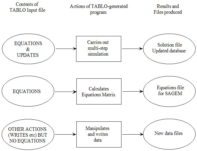
25.1.1 Multi-step simulations with economic models [gpd3.6.1.1]
TABLO Input files for economics models are those containing EQUATION statements. The most important action for the associated TABLO-generated program is that of carrying out a (possibly multi-step) simulation with the model (the first case illustrated in Figure 25.1). This produces a Solution file containing simulation results (percent changes and possibly pre- and post-simulation levels results). It also produces updated data files and other potentially useful files (including Equations and Environment files).
Models with No Update Statements
It should be possible to carry out multi-step simulations with all economic models. This is because the underlying levels equations of an economic model are bound to be nonlinear so that multi-step calculations are required to solve them accurately.
However it only makes sense to carry out a multi-step simulation with models whose TABLO Input files say how the data is to be updated after each step of the calculation (see sections 3.12.3 and 4.4.4). This is why it is not possible to carry out a simulation with TABLO-generated programs whose TABLO Input files contain only linearized EQUATIONs but contain no UPDATE statements or levels VARIABLEs. For these models, the most important action is that of creating the Equations file for the model (see the next section). It is only possible to carry out a Johansen simulation with these models. That must be done by using SAGEM, starting from the Equations file1.
25.1.2 Creating an equations file [gpd3.6.1.2]
If a TABLO Input file contains equations, GEMSIM or the associated TABLO-generated program can be used to create an Equations file. [This is the second case illustrated in Figure 25.1.] You may want to create the Equations file in order to investigate closure or homogeneity problems using SUMEQ (see chapter 79). This Equations file can also be the starting point from which you can carry out Johansen simulations by running the program SAGEM (see 58).
25.1.3 Other actions [gpd3.6.1.3]
Other possible actions are those of doing the
- DISPLAYs (if there are any) in your TABLO Input file — see section 22.3.
- WRITEs (if there are any) in your TABLO Input file — see section 22.1.1.
- ASSERTIONs (if there are any) in your TABLO Input file — see section 25.3.
- TRANSFERs (if there are any) in your TABLO Input file — see section 25.5.
- Range tests (if there are any) in your TABLO Input file — see section 25.4.
These other actions may include "extra" TABLO-like statements on the Command file, including xwrite, xdisplay and xtransfer statements (see section 25.6).
25.1.4 Data manipulation [gpd3.6.1.4]
Sometimes TABLO Input files are created for data manipulation rather than for modelling (see section 38.3 for an example). In this case there are no EQUATIONs (and hence no VARIABLEs or UPDATE statements) and the only possible actions are the Other Actions (WRITEs, DISPLAYs, ASSERTIONs, TRANSFERs or Range tests). [This is the third case illustrated in Figure 25.1.] The WRITEs are usually the main actions since they can produce new (or modified) data files.
If you wish to look at the values of Coefficients and expressions in your data-manipulation TAB file, you can do so via AnalyseGE if you produce a CVL file (see section 28.3).
25.1.5 "extra" (TABLO-like) actions [gpd3.6.1.5]
Note that TABLO-generated programs and GEMSIM are also usually able to carry out some "extra" actions (TABLO-like statements in the Command file rather than in the TABLO Input file) - see section 25.6. Usually these "extra" actions are carried out during the reads/formulas part of step 1 (see Figure 25.2).
25.1.6 Checking the closure and shocks [gpd3.6.1.6]
Another possible action is described in section 24.12, namely that of checking the closure and shocks (without doing a simulation). Section 25.2.1 below tells you when this checking is done.
25.1.7 Postsim passes and actions [gpd3.6.1.6a]
If the program is carrying out one or more multi-step calculations, there may be postsim passes (see 12.5) at the end. These postsim passes are carried out after data is updated. During the postsim part of a run, the relevant actions (Writes, Assertions and Displays) are carried out during postsim pass number 3 (the last of the postsim passes). See section 12.5 for more details.
25.1.8 Controlling whether and how the actions are carried out [gpd3.6.1.7]
Unless you directed otherwise (via the options menu at the start of the CODE stage of TABLO - see section 50.0.1), GEMSIM and/or the TABLO-generated program are capable of carrying out all the actions in the TABLO Input file. When you run either GEMSIM or the TABLO-generated program, it will normally carry out all of these actions.
However you can control whether and how these are carried out. The Command file statements.
neq = yes ; ! don't do equations nwr = yes ; ! do no writes nds = yes ; ! do no displays Assertions = yes|no|warn ; ! see section 25.3 Range test initial values = yes|no|warn ; ! see section 25.4.4 Range test updated values = updated|extrapolated|both|no|warn ; ! section 25.4.4
can be used to stop writes, displays or control how assertions and range tests are carried out.
If you include the statement
simulation = no ; ! don't do simulation
then the equations can be calculated (and the Equations file written) but no simulation is carried out. If you start from an existing Equations file and include this statement, you can still set up and save a closure on an Environment file.
Of course, equations are essential for a simulation and so, if you include
neq = yes ; ! Do no equations
this means that no simulation will be carried out either, and the only actions possible are the "Other actions" (writes etc).
If you include the statement
nud = yes ; ! don't do final updates
the final updated data files are not written (but intermediate ones — see section 25.2 - are calculated since this is essential for calculating a multi-step solution).
25.1.9 Some reads and FORMULAS may be omitted [gpd3.6.1.8]
If you tell the program not to carry out some actions it is capable of (for example, by including the statement "nds = yes ;" in your Command file when the TABLO Input file contains DISPLAYs), the program may not do all READs and FORMULAs in the TABLO Input file. It only does enough to calculate the values of all COEFFICIENTs required to carry out the actions requested. For example, consider the following simple TABLO Input file.
COEFFICIENT C1 ; C2 ; C3 ; READ C1 FROM TERMINAL ; FORMULA C2 = C1 + 1 ; FORMULA C3 = C1 + 2 ; DISPLAY C2 ; WRITE C3 TO TERMINAL ;
If you include "nds = yes ;" in your Command file, the FORMULA for C2 will not be calculated (since the value of C2 only needs to be calculated in order to display it). But if the FORMULA for C3 were changed to
FORMULA C3 = C2 + 1 ;
then the FORMULA for C2 would be executed since its result is required to calculate C3.
This principle is also applied to READs and FORMULAs at steps 2,3... of a multi-step calculation. If the values of some COEFFICIENTs are only needed to calculate entries of submatrices involving a variable which is exogenous and not shocked, the READs and/or FORMULAs for these COEFFICIENTs will not be carried out at steps 2,3... (but they will be at step 1 since the closure is usually not known at that time).
25.1.10 Writes and displays at all steps of a multi-step simulation [gpd3.6.1.9]
Normally WRITEs and DISPLAYs are only done during step 1 of a multi-step simulation (when they reflect values on the original data files). Occasionally, perhaps because you are trying to identify a problem with your UPDATE statements, you may wish to see these values at all steps of the simulation. If you include the statement.
dws = yes ; ! Displays and Writes to terminal at all Steps
in your Command file, all displays and writes to the terminal (but not to Header Array files or other text files) will be done at each step.
25.1.11 Echoing activity [gpd3.6.1.10]
During a run of GEMSIM or a TABLO-generated program, "echoing activity" means indicating all reads, formulas, set, subsets, displays, writes, backsolves and updates as they are carried out, and reporting how many nonzeros are in each submatrix as it is calculated.
If you are carrying out a simulation, the default is to echo activity during the first step only. In this case, if you include the statement.
eaa = yes ; ! Echo All Activity
activity is echoed during all steps of a multi-step simulation.
If you are not carrying out a simulation, the default is to echo all activity. In this case, if you include the statement.
eaa = no ; ! do not Echo All Activity
activity is not echoed.
25.1.12 Writes to the terminal [gpd3.6.1.11]
By default WRITEs to the terminal are done in row order. If you include the statement.
twc = yes ; ! Terminal Writes in Column order
in your Command file, all terminal writes will produce arrays written in column order (that is, col_order) as described in chapter 38.
25.2 How these programs carry out multi-step simulations [gpd3.6.2]
In a multi-step simulation, there is first a preliminary pass (see 32.2), the purpose of which is to work out details of sets and subsets (set size and elements) and set mappings. Some reads and formulas may be carried out during this step, but only those needed to work out sets and subsets.
Then follow the several steps of a multi-step simulation. Each step of a single multi-step simulation consists of the following main parts:
- sets, subsets, reads, writes, displays, assertions, transfers, calculations of formulas, and any "extra" statements. Writes, displays and transfers are done only during the first step. Processing the closure and shocks (see section 25.2.1) is done here during the first step only.
- calculation of equations, one submatrix (see chapter 79) at a time,
- the simulation part (solving the equations),
- backsolving (if required),
- updating the data,
- postsim passes (if necessary — see section 12.5).
(See Figure 25.2 for the first five of these parts, some of which are shown there in a little more detail. Postsim passes are done after the data are updated — see section 12.5 for more details.)
Note that, in each step, all reads and formulas are carried out before any equations are processed. This means that the values of Coefficients in the Equations are those after ALL formulas and reads, not just after all formulas and reads which occur in the TABLO Input file before the equation. See section 11.16.2 for more details.
For a Johansen (that is, a 1-step) simulation, each of the above is done just once. For a single N-step simulation, each is done N times if you are using Euler's method or the midpoint method while each is done (N+1) times if you are using Gragg's method2.
If you are extrapolating on the basis of two or more multi-step solutions, each solution is calculated (first the one with the smaller number of steps, then the one with the next most, and so on).
Finally, the extrapolation is carried out. This involves taking an appropriate linear combination of the different solutions (and updated data bases).
Normally DISPLAYs, WRITEs, TRANSFERs and any "extra" actions are only done during part 1 above of the first step of the first multi-step solution, when values written or displayed reflect values in the original data. [If you are using existing Equations and SLC files, or an LU file, to start the simulation (see sections 59.2 and 59.3), note that 1 and 2 above are not done during step 1, so that DISPLAYs, WRITEs, TRANSFERs and "extra" actions are usually not done.]
An ASSERTION may be done in each step or just in the first step, depending on the qualifier (if any) in the ASSERTION statement in the TABLO Input file. [The qualifier ALWAYS, which is the default, means that the assertion is tested at each step, whereas the qualifier INITIAL means that the assertion is only tested in the first step. See section 10.14.]
Figure 25.2 Calculation of one multi-step solution
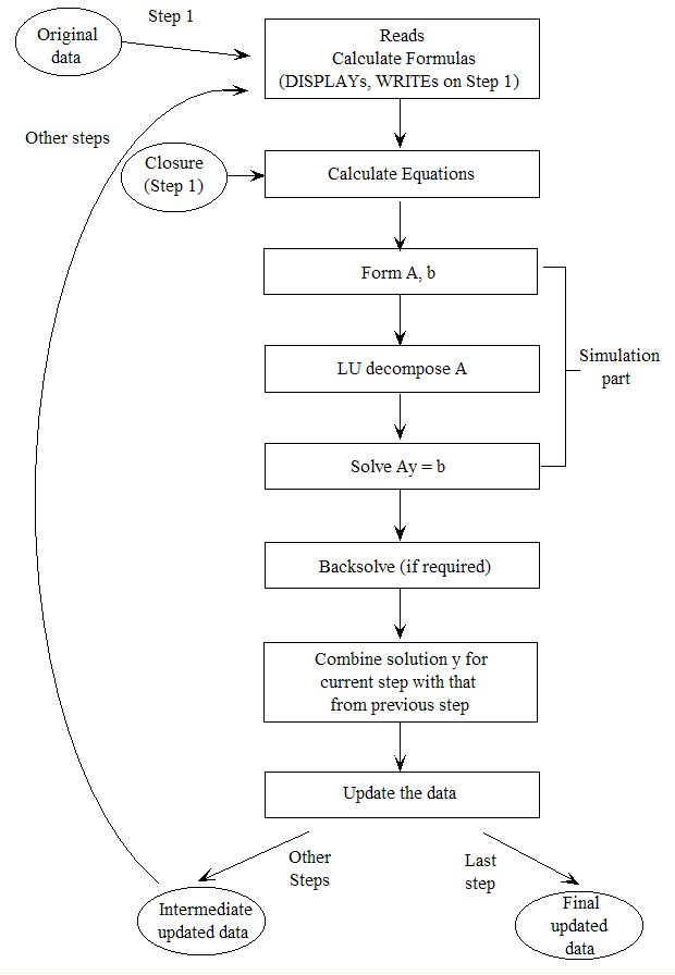
In an N-step simulation, the shocks are broken into N equal parts. In step number K, the formulas and equations are calculated on the basis of the data as updated after step K-1 (if K is at least 2, or the original data if K=1), and the effect of applying just the part of the shock relevant to this step is calculated; this gives a solution, say y(K) for just these shocks. (See below for more explanation as to how y(K) is calculated.) This solution y(K) is added to the combined solution x(K-1) before this step to produce the combined solution x(K) after K steps. [x(K) reflects the movements in the endogenous variables corresponding to just K Nths of the total shocks.] Thus,
x(1) = y(1) step 1
x(2) is obtained from x(1) and y(2)
x(3) is obtained from x(2) and y(3), and so on.
We give a concrete example in section 25.2.2 below.
At the end of each step the data is updated on the basis of the step solution y(K). Specifically, the solutions in y(K) are applied to the updated data after step K-1 to produce the updated data after step K. This data is the starting point for step K+1 (or is the final updated data at the end of this multi-step simulation if this is the last step).
At step K, the linear equations (based on the data at the start of this step) are formed up as
C(K).z = 0
much as in equation (1) of section 3.12.1. Note that, in a multi-step simulation, the Equations Matrix C changes from step to step reflecting the changes in the data as it is updated, which is why we use the notation C(K) above. Then, taking account of the closure and of the shocks for this step, the equations are expressed as
A(K).y(K) = b(K)
much as in equation (3) of section 3.12.2. Here the LHS matrix A(K) and the RHS vector b(K) depend on K as does the solution y(K) for this current step. These equations are solved as described in section 30.1 below: first the LU decomposition of A(K) is carried out (this is the time-consuming part) and then the values of y(K) are calculated. The solution y(K) is normally made as accurate as possible by using iterative refinement (see section 30.1 below).
Note that, if you condensed your model, some backsolving may be done even if you didn't explicitly ask for the values of any eliminated (endogenous) variables to be calculated (see section 14.1.12). These are done if they appear to speed up the updates (which are done after backsolving).
25.2.1 Processing the closure and shocks [gpd3.6.2.1]
GEMSIM and TABLO-generated programs aim to process the closure (the initial check — see section 23.2.7) and the shocks as early as possible. This is done to give you quick feedback on any problems with them. Often
- they process the closure as soon as all SET and SUBSET statements (including any "extra" ones - see section 25.6) have been processed (this usually happens on the preliminary pass - see section 32.2).
- they process the shocks as soon as all SET and SUBSET statements and all WRITEs to text files or to the terminal (including any "extra" ones) have been processed.
If the closure or shocks depend on the value of any Coefficients3, this processing is delayed until the values of these Coefficients are known.
The shocks are delayed until after any write so that it is possible to write a shocks file (eg, a Header Array shocks file) and use it on the same run.
25.2.2 Results of a 4-step simulation looked at in detail [gpd3.6.2.2]
In this section we look at the results of the 4-step version of the simulation carried out in section 20.4 or 3. This is the simulation with Stylized Johansen in which the supply of labor is increased by 10%. We show how the shock for each of the steps is calculated, and show how the final results for certain endogenous variables are built up from the results of the individual steps.
Note that it is not necessary to understand this in order to carry out multi-step simulations with GEMPACK, so you may prefer to skip this section.
The results discussed in this section are those obtained using Euler's method. (Gragg's method or the midpoint method would give different results.)
(a) How the Shock is Broken Up
Imagine that the initial supply of labor is 100 units; we show how the 10% shock to it is broken up into the shock for each of the 4 steps4.
Over the whole simulation, the labor supply must increase by 10%, that is, from 100 to 110, which is an overall increase of 10 units. The shocks at each step are always calculated to ensure that
the same increase (in levels) occurs at each step.
Thus, at each step, the supply must increase by 2.5 (=10/4) units.
In step 1, supply must increase from 100 to 102.5 which is an increase of (2.5/100)x100=2.5%. In step 2, supply must increase from 102.5 (its value after step 1) by a further 2.5 units to 105 units; this is an increase of (2.5/102.5)x100=2.439%. Similarly in step 3 the increase is (2.5/105)x100=2.381%, while in step 4 it is (2.5/107.5)x100=2.326%.
| Step | Supply at start | Increase | Supply at end | % Increase |
| 1 | 100 | 2.5 | 102.5 | 2.5 |
| 2 | 102.5 | 2.5 | 105 | 2.439 |
| 3 | 105 | 2.5 | 107.5 | 2.381 |
| 4 | 107.5 | 2.5 | 110 | 2.326 |
(b) Calculation of Results for Endogenous Variables
Consider first what happens to just one of the endogenous variables, namely p_XH("s1"), as these four partial shocks are applied to the model.
In the first step, it turns out that the levels variable XH("s1") increases by 1.5%.5 For simplicity (again this makes no difference to the final outcome) we suppose that the initial value of the levels variable XH("s1") = 100 as well. After the first step, XH("s1") = 101.5 units.
In the second step, in response to the 2.439% shock to XFAC("labor"), the increase in XH("s1") = 1.463%, the updated value of the levels variable XH("s1") is calculated from
XH("s1") = 101.5 * (1 + 1.463/100) = 102.985 units
an increase in the combined solution of 2.985%.
In the third step, in response to the 2.381% shock to XFAC("labor"), the increase in XH("s1") = 1.429%, and so the levels variable XH("s1") is updated to
XH("s1") = 102.985 * (1 + 1.429/100) =104.457
In the fourth step, in response to the 2.381% shock to XFAC("labor"), the increase in XH("s1") = 1.395%, and so the levels variable XH("s1") is updated to
XH("s1") = 104.457 * (1 + 1.395/100) =105.914
an overall increase in the four steps of 5.914%
Using the notation from section 25.2 above, namely letting y(K) denote the step solution at the Kth step, and x(K) the combined solution after K steps, the results for p_XH("s1") are summarised in the following table.
| Step | y(K) | x(K) | |
| 1 | 1.5 | 1.5 | x(1) = y(1) |
| 2 | 1.463 | 2.985 | x(2) calculated from x(1) and y(2) |
| 3 | 1.429 | 4.457 | x(3) calculated from x(2) and y(3) |
| 4 | 1.395 | 5.914 | x(4) calculated from x(3) and y(4) |
Thus the 4-step simulation result for the variable p_XH("s1") [in response to the 10% shock to XFAC("labor")] is 5.914%. This is the result for the 4-step Euler solution (not the extrapolated solution) on the Extrapolation Accuracy file SJLB.XAC. [The results are shown in section 3.12.3.]
The table below shows the same information for the endogenous variable p_XH("s2").
| Step | y(K) | x(K) | |
| 1 | 1.75 | 1.75 | x(1) = y(1) |
| 2 | 1.707 | 3.487 | x(2) calculated from x(1) and y(2) |
| 3 | 1.667 | 5.212 | x(3) calculated from x(2) and y(3) |
| 4 | 1.628 | 6.925 | x(4) calculated from x(3) and y(4) |
Thus the 4-step Euler simulation for the variable p_XH("s2") [in response to the 10% shock to XFAC("labor")] is 6.925%.
(c) Updates and Values of Coefficients
See sections 4.4.5 to 4.4.7 for numerical details about the effect of Update statements, the values of Coefficients from step to step and the values of the coefficients of the linearized equations from step to step in this 4-step simulation. [In those sections the simulation is based on SJLN.TAB instead of SJ.TAB but the results are essentially identical in these two cases.]
25.2.3 Do the accurate results satify the linear equations? [gpd3.6.2.3]
Consider the simulation with Stylized Johansen from chapter 3. This is the simulation in which labor supply is increased by 10 percent while capital remains fixed. Here we look at the version of this simulation based on the mixed version SJ.TAB of Stylized Johansen. The accurate results of the simulation (obtained by extrapolating from Euler 1,2,4-step calculations) are reported in detail in section 3.7.
There are several linearized equations explicitly in SJ.TAB. Consider for example the equation in the TABLO Input file SJ.TAB for Consumer Demands:
Equation Consumer_demands (All,i,SECT) p_XH(i) = p_Y - p_PC(i) ;.
Is this equation satisfied by the simulation results (as reported in section 3.7)?
Let's try this for the second commodity "s2". The relevant results are
p_XH("s2") = 6.8993
p_Y = 5.8853
p_PC("s2") =-0.9486
p_Y - p_PC("s2") = 6.8339
As you can see, these DO NOT satisfy the linear equation since
the LHS (Left Hand Side) = 6.8993 while the RHS (Right Hand Side) = 5.8853 - (-0.9486) = 6.8339.
This is something that often puzzles new (and some experienced) users. Although the linear equations are solved at each step (and so hold in each step) of a multi-step calculation,
usually they will not be satisfied by the accurate results.
To see why this is the case for the equation above, let's rewrite it by taking the p_PC term to the LHS, when the equation becomes
p_XH("s2") + p_PC("s2") = p_Y ; (1)
In the levels, this says that Y is proportional to the product of XH("s2") and PC("s2"), that is6 :
XH("s2") * PC("s2") = ALPHAH("s2") * Y ; (2)
for some parameter (that is, constant) ALPHAH("s2"). We have seen from the results above that the pre-simulation levels values are
XH("s2") = 4
PC("s2") = 1
Y = 6
and so ALPHAH("s2") must equal 4/6 = 0.6667.
Suppose that the linear equation (1) above were satisfied. Then, given the simulation results p_XH("s2") = 6.8993 and p_PC("s2") = -0 0.9486, you see that
p_Y would equal 6.8993 - 0.9486 = 5.9507
In that case the post-simulation values (given the pre-simulation values and the percentage changes) would be
XH("s2") = 4.2670 (6.8993% larger than 4),
PC("s2") = 0.9905 (0.9486% less than 1) and
Y = 6.3544 (5.9507% larger than 6).
These 3 values do not satisfy the levels equation (2) above since
LHS = 4.2265 while RHS = 4.2363 (since ALPHAH("s2") = 0.6667).
This is one way of seeing that the linear equation (1) should not be satisfied7.
A second way of seeing that the linear equation (1) should not be satisfied is as follows. It is easy to see that the exact percentage change in a product A*B is
p_A + p_B + (p_A*p_B/100)
if p_A and p_B are the percentage changes in A and B respectively8. Thus the exact connection between the linear variables, as derived from levels equation (2), is
p_XH("s2") + p_PC("s2) + [p_XH("s2")*p_PC("s2")/100] = p_Y (3)
This is, of course different from the linearized equation (1) or the linearized equation Consumer_demands in the TAB file, since the term inside the square brackets [] is not included in the linearized equation in the TAB file SJ.TAB9. This is a second reason why the linear equation in the TAB file should not be satisfied by the accurate results.
The thing to take away from this discussion is that it would be a bad thing if the linearized equations were satisfied by the results of the simulation (see the first explanation above). It is a good and desirable feature that the linearized equations are not (in general) satisfied exactly by the accurate percentage change results of a simulation10.
Remember that the aim of the whole simulation is to solve the non-linear levels equations, not to solve the approximate linearized equations (as written in the TABLO Input file)11.
25.3 Assertions [gpd3.6.3]
An Assertion statement requests the software to check conditions you expect to hold.
Assertions are introduced in section 10.14. As explained there, assertions are tested either on the initial (that is pre-simulation) data or else on this and on the updated data produced at each step in a multi-step calculation.
If an assertion is not satisfied, the software tells you the element names (or numbers if names are not available) each time it fails. For example, if the assertion
ASSERTION # Check no negative DVHOUS values # (all,c,COM) DVHOUS(c) >= 0 ;
fails for commodity "wool" you will see the message
%% Assertion 'Check no negative DVHOUS values' does not hold (quantifier number 1 is 'wool')
(and once for each other such commodity 'c' where the assertion fails) and then the message
Assertion 'Check no negative DVHOUS values' does not hold.
By default, if an assertion fails,
- the program stops after informing you of the names of the elements where it fails.
- you can easily see the values of the relevant Coefficients (see section 25.3.1).
You can change this behaviour via the following statement in your Command file.
Assertions = YES|no|warn ; ! default is "yes"
If you include "assertions = no ;", assertions are not checked.
If you include "assertions = warn ;", assertions are checked, but a failure results in a warning only. The first few warnings are shown in detail on the log file. A summary at the end of the run tells you how many assertion failures there have been (if any). You can check if there have been any by searching for "assertion failure" in your log file.
Example from ORANIG01.TAB
In ORANIG01.TAB (see section 60.5.1) are formulas to calculate DIFFIND and DIFFCOM. If the data base is balanced, these values should be zero. However, with the sort of rounding that goes on when arithmetic calculations are done on computers, and remembering that GEMPACK programs only produce results which are accurate to about 6 figures (see section 25.8), it is not reasonable to require that these values are exactly zero. Hence it would be unwise to include the Assertions
Unrealistic assertions
Assertion # DIFFIND values zero # (All,i,IND) DIFFIND(i) = 0 ; Assertion # DIFFCOM values zero # (All,c,COM) DIFFCOM(c) = 0 ;
As you can see from the DIFFCOM(c) values as reported in section 25.8.2, these Assertions would fail. Instead, you will find the following more modest and realistic Assertions in ORANIG01.TAB.
Assertion ! if below not true, program will stop with message ! # DIFFIND = V1TOT-MAKE_C = tiny # (all,i,IND) ABS(DIFFIND(i)/V1TOT(i)) <0.001; # DIFFCOM = SALES-MAKE_I = tiny # (all,c,COM) ABS(DIFFCOM(c)/SALES(c)) <0.001;
It is reasonable to expect that these ratios are small.
25.3.1 When an assertion fails [gpd5.9.7]
If an Assertion fails, you will see, on the terminal and on the LOG file (if you produce a LOG file)
- the list of quantifier values for which the assertion fails.
- a closing statement indicating that the Assertion failed.
The values of all Coefficients (or Variables) that occur in the Assertion are written to a special Header Array file so that you can look at the relevant values. We hope that this will make it easier for you to understand why your Assertion failed.
-
If you are carrying out a simulation, the name of this Header Array file
is
<SL4-name>-ASSERT-FAIL.HAR
where <SL4-name> is the name (excluding suffix) of the Solution file. -
If you are not carrying out a simulation, the name of this Header Array file
is
GP<xxx>-ASSERT-FAIL.HAR
where <xxx> will be replaced by something like XX1 or X23. The LOG file will include the exact name of this Header Array file.
The different Coefficients and Variables will be written to different headers. The long name associated with each header will tell you which coefficient and which assertion the values relate to.
Example: Consider the following Assertion.
Assertion # Coeff1+Coeff2 <10 # (all,c,COM) coeff1(c)+coeff2(c) <10;
Suppose that this fails when c="c2" and also when c="c3". Then, in the LOG file for this run, you will see something like the following.
%% Assertion 'coeff1+coeff2 < 10' at line number 642 does not hold when quantifier is "c2". %% Assertion 'coeff1+coeff2 < 10' at line number 642 does not hold when quantifier is "c3". (Written real array, size 3, header '0003'.) (Written real array, size 3, header '0004'.) [Have written coeff/var values to headers "0003" to "0004" of file "gpxx1-assert-fail.har".] Assertion 'Coeff1+Coeff2 <10' at line number 642 does not hold.
The values of Coefficient COEFF1 are written to header "0003" and the long name at that header is "Values of coeff1 in assertion coeff1+coeff2 < 10". The last part of this is taken from the labelling information (between # and #) for the Assertion.
The values of Coefficient COEFF2 are written to header "0004".
Note that the line number of the Assertion in the TAB file is indicated in the log file output. This can be helpful if the TAB file contains several similar assertions.
25.3.2 Assertions, writes on preliminary pass and PostSim pass 2 [gpd5.9.8]
25.3.2.1 Assertions and writes to terminal may be done on preliminary pass [gpd5.9.8.1]
GEMSIM and TABLO-generated programs always do a Preliminary pass in order to work out sets, subsets and set mappings (see section 32.2 for details).
- Writes to the terminal (not to other places) are carried out during the Preliminary pass provided at least some values have been given to the Coefficient being written on the Preliminary pass.
- Assertions are carried out during the Preliminary pass provided that at least some values have been given to all of the Coefficients involved in the Assertion on the Preliminary pass.
These Writes and Assertions will also be done again on the first actual pass.
Coefficients are only given values on the Preliminary pass if their values are needed in order to work out the elements of a data-dependent set (see section 10.1.3) or a set mapping.
Example. Consider the following TAB file.
file input ;
set com read elements from file input header "COM" ;
coefficient (all,c,com) coef1(c) ;
coefficient (all,c,com) coef3(c) ;
read coef1 from file input header "c1" ;
read coef3 from file input header "c3" ;
! Next SHOULD be done on Preliminary pass !
assertion # check COEF1 values# (all,c,com) coef1(c) > 0 ;
write coef1 to terminal ;
! Next should NOT be done on Preliminary pass !
assertion #check COEF3 values# (all,c,com) coef3(c) > 0 ;
write coef3 to terminal ;
! Values of COEF1 will be worked out on Preliminary
pass because of next statement !
set scom1 = (all,c,com: coef1(c) > 1) ;
write (all,c,scom1) coef3(c) to terminal ;
The set SCOM1 is a data-dependent set. Hence the values of Coefficient COEFF1 will be worked out on the Preliminary pass. But the values of Coefficient COEFF3 will not be worked out on the Preliminary pass. Hence the Assertions and Writes to the terminal involving COEFF1 will be done on the Preliminary pass but not those involving COEFF3.
25.3.2.2 Assertions and writes to terminal may be done on PostSim pass 2 [gpd5.9.8.2]
When there are PostSim statements, sets and subsets declared in the PostSim part of the TAB file are worked out on the second PostSim pass (see section 12.5).
- Writes to the terminal (not to other places) are carried out during PostSim pass 2 provided that at least some values have been given to the Coefficient begin written on PostSim pass 2. This applies to both normal and PostSim Coefficients.
- Assertions are carried out during PostSim pass 2 provided that at least some values have been given to all of the PostSim Coefficients involved in the Assertion on PostSim pass 2. [Any normal Coefficients occurring always have values - their updated values - by this stage.]
These Writes and Assertions will also be done again on PostSim pass 3 (the final PostSim pass).
Note that PostSim Coefficients (those declared in a PostSim part of the TAB file) are only given values on PostSim pass 2 if their values are needed in order to work out the elements of a data-dependent PostSim set (see section 12.5). The values of ordinary Coefficients (those not declared in a PostSim part of the TAB file) are always available during PostSim pass 2 since their values (updated values) are set up on PostSim pass 1.
25.4 Range tests [gpd3.6.4]
Coefficients and levels variables may naturally have a certain range of acceptable values. For example, Coefficients representing dollar values should always be at least zero.
When Coefficients or Levels Variables are declared in the TABLO Input file, qualifiers such as (GE 0) can be used to specify acceptable ranges of values for them (see sections 10.3, 10.4 and 10.19.1). For example
Coefficient (GE 0) (All,c,COM) DVHOUS(c) ;
These range tests are carried out when GEMSIM or the TABLO-generated program runs. They affect the run of the program in the following two ways.
- When the data is read or updated, tests are carried out to check if the values are in the specified range. A run-time error will normally occur if one or more of the values is outside the acceptable range.
- If you are carrying out a simulation using user-specified accuracy (often called automatic accuracy - see section 26.4), the software uses these tests to decide if the current subinterval length is too large. [If one or more updated values are outside the specified range, the software automatically repeats the current subinterval, using a shorter subinterval length.]
Specifying acceptable ranges, and having the software carry out these range tests, ensure that you will not report simulation results based on a run where one or more of the pre-simulation or updated values is outside its acceptable range.
The typical case that motivates this is where some sector is declining as a result of the simulation, so that the level of its output is getting smaller, possibly close to zero (as in Figure 25.3). In such a case, the straight-line approximations used in Euler's method (or Gragg or midpoint) can cause the output level to become negative after one or more steps. [In Figure 25.3, the 2-step Euler result over the subinterval shown is indeed negative.]
If this happens, the software realises as soon as it updates the value to be negative that this should not happen.
- If you are using user-specified accuracy (see section 26.4), which means that the program is controlling the subinterval length, the program abandons the current subinterval and does it again, this time with a shorter subinterval length. The basic idea is that the software uses this extra information about the coefficients to make sure that subintervals are not too long.
- If you are not using user-specified accuracy (that is, you have specified the number of subintervals and the number of steps in each subinterval), the software will report the error (it will say which parts of which coefficient have gone out of range) and will then normally stop with an error. In this case you will need to rerun the simulation choosing more subintervals and/or steps.
Figure 25.3 Levels value can become negative if subinterval is too long
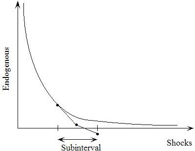
25.4.1 Specifying the allowed range for a coefficient or levels variable [gpd3.6.4.1]
This may be done when you declare the Coefficient or Levels Variable in your TABLO Input file (see sections 10.3, 10.4 and 10.19.1). You can use Coefficient or Variable qualifiers which specify acceptable range of values. For example,
Coefficient (GE 0) (all,c,COM) DVHOUS(c) ; Variable (Levels, GE 0) (all,c,COM) DVHOUS(c) ;
Either of these specifies that DVHOUS(c) values should always be at least equal to zero.
When such a qualifier is used with a Levels Variable, the range restriction actually applies to the Coefficient automatically associated with this Levels Variable (see section 9.2.2).
Allowed qualifiers are of the form
<operator> <real-number>
where <operator> must be one of GE,LE,GT,LT or their symbol
version
| GE | or | >= |
| LE | or | <= |
| GT | or | > |
| LT | or | < |
and <real-number> can be any real number (with or without a decimal point).
For example,
GE -1.1 LT 10
At most two such qualifiers are allowed with each declaration, namely at most one of GE,GT and at most one of LE,LT. [For example, the two qualifiers (GE 0, GT -1) are not allowed since one or other would be redundant.] An example with two such qualifiers is
Coefficient (GE 0, LE 1) (all,c,COM) SHARE(c) ;
These qualifiers given in brackets after the keyword "Coefficient" can only be attached to REAL Coefficients; they cannot be attached to INTEGER Coefficients.
We suggest that, normally, these qualifiers should be attached to Coefficients which are READ and/or UPDATEd (though the software allows them to be attached to any Coefficients).
Of course they can also be attached usefully to any Levels Variable (since these are always updated - see section 9.2.2).
Default ranges may apply — see section 10.19.1. If, for example, you have many Coefficients which should be at least zero, you can put the statement
Coefficient(Default=LOWER_BOUND GE 0) ;
before the declarations of these Coefficients. Then you can include the statement
Coefficient(Default=LOWER_BOUND OFF) ;
to turn off the default if relevant.
25.4.2 Tests carried out [gpd3.6.4.2]
Test of Initial Values
These range qualifiers are used to test the values of the Coefficient in question at the end of the reads, formulas etc on the first step of the first subinterval of a simulation. [Note that the testing is not done immediately some or all of the values of the coefficient are read or assigned via a formula. The testing is only done once all reads and formulas are done.]
All Coefficients are tested even if one fails.
If one or more fails, the program stops after all of the reads, formulas etc.
This testing is always carried out, even if user-specified accuracy is not being used.
For these tests, the range qualifiers act similarly to ASSERTIONs which are tested only on the first step of the first subinterval.
(b) Test of Updated Values
These range qualifiers are used to test the UPDATEd values of the coefficient in question (at each step and whenever its values are extrapolated).
If an updated value falls outside the specified range,
the current subinterval is redone with a shorter length if user-specified accuracy (26.4) is being used. In this case the simulation continues.
a warning is normally given if user-specified accuracy is not being used — see section 25.4.4 for details.
25.4.3 An example [gpd3.6.4.3]
Consider the experiment called E1 in the GTAP application about abolishing the Multi-Fibre Agreement (see chapter 10, written by Yongzheng Yang, Will Martin and Koji Yanagishima, of the GTAP book, Hertel (1997)). This is supplied in the GEMPACK examples as Command file GC10E1.CMF.
Implement GTAP61 as described near the start of section 26.1.1.
Case 1. Range Errors Produce Only Warnings
Look at the Command file GC10E1.CMF. You will see that this extrapolates from Gragg 4,6,8-step calculations over one subinterval ("subintervals = 1 ;").
Run this simulation using Command file GC10E1.CMF. Check the LOG file GC10E1.LOG produced. Notice the following lines at the end of the LOG file.
(The program has completed without error.) (There were 2 warnings.) (If you have a LOG file, search for '%%W' to see them.) (The last was:. 'Updated value out of range')
The last reported warning "Updated value out of range" should suggest a problem to you.
Notice also, a few lines above, near the end of the LOG file, the lines
%%WARNING. There have been 5 range-check warnings. [Search for '%% Test that ' in your log file to see the first few of each type of these warnings.] These warnings relate to the following types of values: Updated
Go to the top of the LOG file and search for "%% Test that" as suggested. The message at the first occurrence is
%% Test that updated values of VIMS GE 0 fails (Value is -3.7447128) (quantifier number 1 of coefficient 'VIMS' is 'CLG') (quantifier number 2 of coefficient 'VIMS' is 'AUS') (quantifier number 3 of coefficient 'VIMS' is 'NAM')
From just above this in the LOG file, you can see that this happens during pass 3 of a 5-pass calculation. [This is during the 4-step Gragg calculation which actually does 5 passes or calculations — see section 30.2.] This warning is given since Coefficient VIMS is declared in GTAP61.TAB via the statement
Coefficient (ge 0)(all,i,TRAD_COMM)(all,r,REG)(all,s,REG)
VIMS(i,r,s) # imports of i from r to s valued at domestic mkt prices #;
The qualifier "(ge 0)" indicates that the values of this Coefficient should never be negative.
If you continue to search in the LOG file for "%% Test that" you will see other instances of Coefficients going out of their expected ranges12.
Despite all of this, the simulation has completed without error. This is because (as is documented in section 25.4.4 below) the default is to give only warnings when a Coefficient goes out of range. If you think this is unsatisfactory, you can turn these warnings into fatal errors (as perhaps they should be by default) by putting the statement
Range test updated values = both ;
into the Command file. We have done this in Command file GC10E1RT.CMF (where the "RT" indicates "Range Testing") — see Case 2 below.
Case 2. Range Errors Are Fatal Errors
Look at the Command file GC10E1RT.CMF. The only difference between this Command file and GC10E1.CMF used above is that the statement "Range test updated values = both ;" has been added.
Run the simulation using Command file GC10E1RT.CMF and check the LOG file GC10E1RT.LOG. You will see that the simulation ends with an error. The following messages are near the end of the LOG file.
Updated values of at least one coefficient are not in the required range. (See the earlier message(s) referring to "test that updated value".) (ERROR RETURN FROM ROUTINE: Main Program) (E-Updated value out of range)
If you go to the top of the LOG file and search for "test that updated value" you will see that there are 5 reports of values of Coefficients going out of range.
What can you do to fix up this problem? You could try to increase the numbers of steps until (hopefully) nothing goes out of range. That would work if you took enough steps13.
However, a simpler way around this problem is to let the software do the hard work. You can do this by specifying automatic accuracy (see section 26.4), which we ask you to do in Case 3 below.
Case 3. Automatic Accuracy
Look at the Command file GC10E1AA.CMF (where "AA" indicates "Automatic Accuracy"). The only difference between this Command file and GC10E1.CMF used in Case 1 above is that the statement
Automatic accuracy = yes ;
has been added.
Run the simulation via Command file GC10E1AA.CMF and check the LOG file GC10E1AA.LOG. You will see that the simulation completed without error. The LOG file indicates that there was 1 range-check warning. If you go to the top of the LOG file and search for "%% Test that" you will see that the values of VIMS("CLG","AUS","NAM") went out of range as before. But this time all that happens is that the program now takes responsibility and redoes the subinterval with a shorter length. Accordingly, this simulation is now completed in 2 subintervals. [To see this, go to the top of the LOG file and search for "++>". You will see that subinterval 1 is redone with length 0.6, which completes satisfactorily without any Coefficient going out of range. Then subinterval 2 has length 0.4 of the whole simulation.]14.
Clearly using automatic accuracy is the best alternative for this simulation. Then the software can ensure that the values of all Coefficients stay in the range required by the "(ge 0)" qualifiers associated with many of the Coefficients in GTAP61.TAB.
This example is a good illustration of the value of specifying acceptable ranges of values for the Coefficients in your model. It is especially powerful when used in conjunction with automatic accuracy15. In general, if a simulation shows range test warnings, either increase the numbers of steps until the warnings disappear or else (a better way usually) use automatic accuracy.
You may have noticed the statement
Start with MMNZ = 210000 ;
in the Command file GC10E1.CMF. See section 32.3 for details about this.
25.4.4 Associated statements in command files [gpd3.6.4.4]
The following statements can be used to control which initial and updated values range tests are applied to.
range test initial values = yes|no|warn ;
[For example, if you don't want range testing of initial values, put the statement "range test initial values = no ;" in your Command file.]
range test updated values = updated|extrapolated|both|no|warn ;
Here
- updated only tests values when a coefficient has been updated (but not after extrapolation).
- extrapolated only tests values immediately after extrapolation (but not after updating).
- both tests values at both times (updated and extrapolated).
- no turns off both sorts of tests.
- warn outputs a warning for the first few instances, but the simulation carries on as if these warnings had not been given (that is, as if "no" had been selected).
The defaults and meanings of these are slightly different depending on whether or not automatic accuracy is being done. Details about these statements in the automatic accuracy case can be found in section 26.4.5.
When not doing automatic accuracy
When you are not using automatic accuracy, the default value is "WARN" in each case.
When not doing automatic accuracy, if one of the values is out of range,
- if the relevant "range test ..." is set at "WARN", then a warning is shown for the first few instances but the simulation carries on as if these warnings were not given.
- if the relevant "range test ..." is set at "YES", then the simulation ends with a fatal error after the value out of range is shown (in the log file). Possibly several out-of-range values of the same type (initial, updated or extrapolated) may be shown before the program stops.
- if the relevant "range test ..." is set at "NO", the relevant testing is not done.
We recommend that you set these to "YES" so that you do not report simulation results in which a value goes out of range. [If a value goes out of range, you can increase the number of steps or use automatic accuracy to keep the values in range.]
- If "range test updated values = both ;", then both updated and extrapolated values out of range are fatal errors.
- If "range test updated values = updated ;", then updated values out of range are fatal errors, and the software merely warns about extrapolated values out of range.
- If "range test updated values = extrapolated ;", then extrapolated values out of range are fatal errors, and the software merely warns about updated values out of range.
The only difference between setting one of these to "NO" or to "WARN" is that in the latter case you see individual warnings (giving the actual value and the arguments if relevant) in the log file.
If any range checks are set to be warnings only, a summary at the end tells how range check failures there have been (if there are any). You can check if there have been any by searching for "not in the required range" in your log file.
25.5 Transfer statements [gpd3.6.5]
Full details about TRANSFER statements in TABLO Input files and their operation when GEMSIM and TABLO-generated programs run can be found in sections 10.15 and 11.13. You can use XTRANSFER statements in your Command file, as explained in section 11.13.1.
25.6 TABLO-like statements in command files [gpd3.6.6]
When running GEMSIM or TABLO-generated programs, you can put TABLO-like statements in Command files to
- declare SETs,
- make SUBSET declarations,
- declare extra logical FILEs,
- carry out extra WRITEs, DISPLAYs or TRANSFERs.
These extra statements are carried out as if they were appended to the end of the original TABLO Input file. In each case the syntax and semantics are identical to that in TABLO Input files except that
- keywords are as in TABLO Input files except that an 'X' (for eXtra) is added at the start. That is, the keywords for these statements in Command files are XSET, XFILE, XSUBSET, XWRITE, XTRANSFER and XDISPLAY.
- each statement must start with a keyword.
- there must be at least one space after the keyword before a qualifier. [For example, "xfile(new)" will not be recognised and should be rewritten as "xfile (new)".] See section 25.6.2 below for more details.
- the Command file syntax for comments (rest of line after single '!' is a comment — see section 20.7) is used instead of the TABLO Input file syntax for comments (in which text between two exclamation marks ! is a comment — see section 11.1.4). [TABLO-like comments consisting of text between two exclamation marks '!' or between strong comment markers '![[!' and '!]]!' (see section 11.1.5) are not allowed in extra statements on Command files.]
There are two main reasons why we allow these statements on Command files.
(1) To allow you - without having to rerun TABLO - to examine the values of some COEFFICIENT which you did not write or display in the original TABLO Input file. You can now put XWRITE and XDISPLAY statements in your Command file to do this. For example in Stylized Johansen, to examine the values of coefficient ALPHAFAC, the following statements could be added to the Command file SJLB.CMF (see Figure 3.8.1):
xfile (new,text) sjout ; xwrite alphafac to file sjout ; file sjout = SJLBOUT.DAT ;
See also the use of xwrite statements in the examples in section 25.8.2 below.
(2) To allow you to define SETs which may be useful in specifying the closure or shocks in your simulation. These sets may not be important for the model in general (hence are not defined in the TABLO Input file), but may help you to specify a closure or shocks needed in some simulation.
For example, consider the Command file statements:
xset SPCOM (sheep, cars, services) ; xsubset SPCOM is subset of COM ; modify closure from file xxx ; exogenous x1(SPCOM) ; endogenous x2(SPCOM) ;
These statements set up a closure in which certain components (those in the newly-defined set SPCOM) of variable 'x1' are made exogenous, being swapped for the corresponding components of variable 'x2'.
For an example relating to shocks, look at the Command file GSEFTA1.CMF (supplied with the GEMPACK examples — see section 60.7.1). This Command file contains the statements
! Shocks
XSet AG_COMM # Agricultural commodities # (agric, food) ;
XSubset AG_COMM is subset of TRAD_COMM ;
XSet NONAG_COMM = TRAD_COMM - AG_COMM ;
Shock tms(NONAG_COMM, "safrica", "eunion") =
select from file gtmsa7x5.shk ;
The sets AG_COMM and NONAG_COMM are used when specifying the shocks. See section 24.2 for the meaning of "select from". [In this simulation, the European Union "eunion" is only eliminating import tariffs on non-agricultural commodities imported from South Africa "safrica". Here the text file gtmsa7x5.shk (using a Header Array file would be more modern practice) contains the shocks needed to completely eliminate all import tariffs on all commodities for all regions.]16
In general you can not read data using extra statements in Command files. The one exception is that you can read in set element names and numbers for new sets and subsets. The following example defines a new set "WoolGrain" and then uses it to modify an existing closure.
xfile extraset ; xset WoolGrain # Wool and Grain commodities # maximum size 4 read elements from file extraset Header "WOGR" ; xsubset WoolGrain is subset of COM ; file extraset = EXTRASET.DAT ; modify closure from..... swap f5dom(WoolGrain) = x0(WoolGrain,"domestic") ;
25.6.1 TABLO-like checks of extra statements [gpd3.6.6.1]
In the example above, the declaration of the file extraset (by the XFILE statement) must precede the set statement reading elements from this extraset file. This follows the usual rule that in TABLO, everything must be declared before it is used.
The TABLO-like statements are processed in the same order as they are given in (as if they were appended to the end of the original TABLO Input file). The TABLO-like extra statements are checked for syntax and semantic errors. Errors are reported to the terminal just as they are from the Check stage of TABLO (see section 9.1). Since there is no Information file, they are reported in the LOG file. Error messages refer to the TABLO-like statements as "extra" statements. After this TABLO-style check, if there are no errors, the remaining Command file statements are processed in the usual way.
25.6.2 Qualifiers [gpd3.6.6.2]
In TABLO Input files, a space after the keyword before a qualifier is not necessary. For example, either of the following is allowed.
File (New) output # Summary output # ; File(New) output # Summary output # ;
But, in TABLO-like statements on Command files (see section 25.6), at least one space is required after the keyword before the qualifier. Thus, for example,
Xfile (New) output # Summary output # ;
is allowed but
Xfile(New) output # Summary output # ;
will result in an error.
25.6.3 Other points [gpd3.6.6.3]
The extra statements (XSET, XFILE, XSUBSET, XWRITE and XDISPLAY) only allow you to examine coefficients already defined in the TABLO Input file. Note that they do not allow you to declare new coefficients or variables or to add extra formulas or equations. Nor do they allow you to read extra data (except that they do allow you to read set element names and subset numbers for new sets and subsets, as in the example above). In particular, data-dependent sets (see section 10.1.3) are not allowed as extra statements since these are implemented rather like Formulas (which are not allowed as extra statements).
Note that TABLO-like statements are not allowed on a Command file when you start a simulation from existing Equations and SLC files (via a "use equations file ... ;" statement — see section 59.2.1). This is because, when you start from existing an Equation file, the original data is not read, nor are writes nor displays carried out; hence there is no opportunity to carry out extra TABLO-like statements.
25.7 Coefficients are fully initialised by default [gpd3.6.7]
When you declare a Coefficient, TABLO-generated programs and GEMSIM set all values of the Coefficient to zero by default.
You can change this default if you wish, by including a statement of the form
initialise|initialize coefficients = YES|no|<value> ;
in your Command file (either spelling of 'initialize' is accepted).
- The default YES means that all values of all coefficients are initialised to zero.
- Option "no" means that Coefficient values are not initialised.
- If you wish to initialise all Coefficients to some value different from zero, you can specify the value in the statement. For example,
initialise coefficients = 23.1 ;
will result in all values of all Coefficients being initialised to the value 23.117.
To see the difference consider the following TABLO Input file.
Set COM (c1-c3) ;
Set IND (i1-i4) ;
Coefficient (All,c,COM)(All,i,IND) DVCOMIN(c,i) ;
File FID ;
Read (All,i,IND) DVCOMIN("c1",i) from file FID Header "DVC1" ;
Read (All,i,IND) DVCOMIN("c2",i) from file FID Header "DVC2" ;
Write DVCOMIN to terminal ;
There is no READ or FORMULA setting the values of DVCOM("c3",i) for i in IND.
TABLO will not warn that the DVCOMIN("c3",i) values may not be fully initialised18. So, when the Write statement is carried out, the DVCOMIN("c3",i) values will be different depending on whether or not a statement "initialise coefficients = ... ;" is included on the Command file.
If no such statement is included (or if "initialise coefficients = yes ;" is included), these DVCOMIN("c3",i) values will be zero. [In these cases, the program behaves as if there were the statement
Formula (All,c,COM)(All,i,IND) DVCOMIN(c,i) = 0 ;
after the declaration of Coefficient DVCOMIN.]
If a statement "initialise coefficients = <value> ;" is included, these DVCOMIN("c3",i) values will be equal to <value>.
If a statement "initialise coefficients = no ;" is included, these DVCOMIN("c3",i) values will not be really determined. The relevant memory in the computer will contain random (that is, unpredictable) values.
At present TABLO gives no warning about possibly uninitialised coefficients if two or more partial initialisations are made. If no attempt is made to initialise a coefficient, TABLO will still give an error message. Full details about the way TABLO handles this issue can be found in section 11.11.5.
25.8 How accurate are arithmetic calculations? [gpd3.6.8]
As is well known, computer arithmetic is not completely accurate; for example 10/2 may return 4.9999999.... The size of these rounding errors depends on the size of (or amount of space used by) real numbers in a particular program.
- Many programs (such as Excel or GAMS) use 8 bytes (64 bits) to store a real number in memory or on disk. These 8-byte real numbers (also called "double-precision" reals) are accurate to around 16 decimal digits — so usually, rounding errors are un-noticeable.
- The HAR files used by GEMPACK use 4 bytes (32 bits) to store a real number. These 4-byte real numbers (also called "single-precision" reals) are also used internally by the GEMPACK programs. They are accurate to 6 or 7 decimal digits (1 part in 10 million) — so often, rounding errors are noticeable. However, compared to double-precision, single-precision data handling is twice as quick and uses half the memory or disk space. This allows us to run bigger, more detailed, models.
Economic data from statistical agencies is accurate, at best, to 1%. The elasticities which greatly affect economic models are estimated to within, at best, 10% accuracy. Conclusions or predictions from a model can scarcely be more accurate than this. That is why the GEMPACK developers have chosen to use single-precision reals19.
In single-precision arithmetic 2.0000001 is the same as 2.0 (because the "1" is the 8th decimal digit, and single precision only supports 6 or 7 decimal digits). Since errors accumulate, GEMPACK results are accurate to around only 6 decimal digits.
Could you construct an economic model, solved in double precision, where your predictions or policy conclusions were crucially altered according to whether a certain elasticity had value 2.0000001 instead of 2.0 ? We suggest that in such a case either the model or the interpretation of its results is not sensible, and should be revised. So we see no strong need for double-precision arithmetic, which is slower and uses more memory.
ViewHAR and ViewSOL let you choose to display up to 6 decimal places (ie, digits after the point). But you should understand that, if you choose 6 decimal places to display the numbers
19607.058594.
0.000032
- the first number shows 11 decimal digits — but only the first 6 or 7 mean anything. The "8594" are random digits.
- the second number shows only 2 decimal digits (discard leading zeros) — so could usefully be displayed with more accuracy.
To see numbers with appropriate precision, the ViewHAR and ViewSOL "decimal places" list box offers 3 more options:
- for comfortable viewing, the "flex" option shows up to 3 decimal places (fewer for big numbers).
- the "accflex" and "sci" (scientific) options always show 7 decimal digits — the maximum supported by single-precision arithmetic.
Below we give two examples which illustrate rounding errors.
25.8.1 Example 1 - GTAPVIEW [gpd3.6.8.1]
The standard GTAP TAB file referred to as GTAPVIEW provides a summary of any GTAP data set. We have provided GTPVEW61.TAB with the GEMPACK examples (see section 60.7.1). To see the GTAPVIEW summary of the ACORS3X3 GTAP data set (these are the starting data files for the simulation in section 26.1.1), first run TABLO on GTPVEW61.TAB to produce output for GEMSIM, then run GEMSIM taking inputs from Command file GTPV3X3.CMF (which is discussed in section 22.1.1). This produces two output Header Array files called GTPV3X3.HAR (contains summary totals, shares etc) and GTPV3X3T.HAR (contains tax rates).
There is a lot of interesting information in the output file GTPV3X3.HAR. Please open this with ViewHAR. Look at the data at headers AG01 and AG02. These provide a breakdown of GDP in each of the 3 regions, from the expenditure side (AG01) and the income (or sources) side (AG02). The row totals are the values of GDP for the regions. An important balance check is that GDP for any region should be the same from the two sides.
Check this for the first region SSA (Sub-Saharan Africa). Choose 6 decimal places in ViewHAR. You should see exactly the same total 316125.296875 at both headers, which is excellent balance.
What about for the second region EU? You should see that the value of GDP from the expenditure side is shown as 8208662.000000 while the value from the income side is shown as 8208663.750000. Is this apparent lack of balance serious? No, since you need to always remember that GEMPACK programs only calculate results accurately to about 6 figures. In this large number 8208662, the "2" is the seventh figure. So these two numbers agree to 6 figures, which is all you can expect. Hence the apparent discrepancy is not at all serious. Note also the difference between 6 figures (as explained above) and 6 decimal places. In the large numbers above, the sixth decimal place is the thirteenth figure.
The file GTPVEW61.TAB is an interesting example of a TAB file. For example, look at the set GDPEXPEND and at how the values in Coefficient GDPEXP are built up via several Formulas. This shows a neat way of arranging summary data into Coefficients and hence onto headers on a Header Array file. You may be able to adapt some of these techniques in your own work.
GTAPVIEW with Updated Data
You could also use GTPVEW61.TAB to check that GDP values from both sides are still equal in the updated data after any simulation with GTAP61.TAB. For example, you might like to try this for the GEX15.CMF simulation described in section 26.1.1. As with SJLBCHK.CMF (see section 6.3.2), you just need to change the statement in GTPV3X3.CMF (see section 22.1.1) which tells which GTAPDATA file to read (and you should change the name of the Command file, perhaps to GTPVW-GEX15.CMF).
25.8.2 Example 2 - checking balance of ORANIG data [gpd3.6.8.2]
ORANI-G does not provide a separate TAB file for checking the balance. Instead the relevant calculations have been included in ORANIG01.TAB and are normally carried out each time you do a simulation with ORANI-G. It is easy to carry out just these calculations without doing a simulation, as we show here.
First we look at the following statements in ORANIG01.TAB (see section 60.5.1) which check some parts of the balance of an ORANI-G data set.
Coefficient ! coefficients for checking ! (all,i,IND) DIFFIND(i) # COSTS-MAKE_C : should be zero #; (all,c,COM) DIFFCOM(c) # SALES-MAKE_I : should be zero #; Formula (all,i,IND) DIFFIND(i) = V1TOT(i) - MAKE_C(i); (all,c,COM) DIFFCOM(c) = SALES(c) - MAKE_I(c); Write ! we file these numbers BEFORE the assertions below ! DIFFIND to file SUMMARY header "DIND"; DIFFCOM to file SUMMARY header "DCOM";
For example, DIFFCOM calculates the difference between two separate measures of the total sales of each commodity. As you can see from the TAB file, SALES(c) is obtained by adding up across intermediate use, capital creation, domestic use, exports, government use and stocks while MAKE_I(c) is obtained by adding the value of commodity c produced by each of the industries (as obtained from the MAKE matrix). If the data base is balanced, the DIFFCOM(c) values should be all zero, as should the DIFFIND(i) values for all industries i. Below we show you how to check this for the ORANIG data base contained in Header Array file OGOZD867.HAR.
The first step is to copy the relevant files (ORANIG01.TAB, OG01GS.STI, OG01SUM.CMF and ORANG867.HAR) from the GEMPACK examples folder to a new folder, say C:\ORANIG (or just copy O*.* to C:\ORANIG).
Command-prompt method
Type in the commands below:
cd \ORANIG tablo -sti og01gs.sti gemsim -cmf og01sum.cmf viewhar summary.har
which
- Change into the directory in which the ORANIG01 files are located (say, C:\ORANIG).
- Run TABLO on ORANIG01.TAB using the GEMSIM STI file OG01GS.STI.
- Run GEMSIM taking inputs from the Command file OG01SUM.CMF
- Open the output SUMMARY file called SUMMARY.HAR in ViewHAR.
WinGEM method
Start WinGEM and make sure that both default directories point to the directory in which you put the ORANIG01 files.
First run TABLO on ORANIG01.TAB using Stored-input file OG01GS.STI. To do this, after selecting TABLO Implement from the Simulation menu, click on the Options menu item on the TABLO form, and select item Run from STI file . Then click on the Select button on the TABLO form and select Stored-input file OG01GS.STI, which produces output for GEMSIM. Then click on the Run button. When this run finishes, click on the Go to GEMSIM button.
Then run GEMSIM by selecting Command file OG01SUM.CMF and then clicking on the Run button. When the run has finished, click on the View Input/Output Files button, select the output Summary file which is called SUMMARY.HAR and click OK.
Examining the results
Using ViewHAR, look at the DIFFCOM results at header "DCOM" in SUMMARY.HAR. Are these values all zero?
You will see the DIFFCOM(c) values are not all identically zero, though they are small. For example, the value for commodity number 4 MiningExport is 0.013672. As with GTAP (see section 25.8.1), this is nonzero because of the accuracy limitations (and does not mean that the data is unbalanced). To see this, note that DIFFCOM(c) is calculated as the difference between SALES(c) and MAKE_I(c). We need to see these values but, unfortunately, the values of these Coefficients are not written on the SUMMARY file.
Luckily, the SALES and MAKE_I (and the DIFFCOM) values are available on another file called OG01SUM.CVL20. Use ViewHAR to examine this file (select 6 decimal places). Note that the value of SALES("MiningExport") is displayed as 19607.058594, while MAKE_I("MiningExport") is shown as 19607.044922.
Now we can understand why DIFFCOM("MiningExport") is not exactly zero. As you have seen, this value of 0.013672 is calculated as the difference between 19607.058594 and 19607.044922. These two numbers agree to 6 figures (the sixth figure is the "0" just after the decimal place) but differ in the seventh figure (5 versus 4). Since the values of SALES("MiningExport") and MAKE_I("MiningExport") can only be relied on to be accurate to about 6 figures, you should not be disturbed by the fact that they differ at the seventh figure. Hence you should not be disturbed by the fact that DIFFCOM("MiningExport") is a sufficiently small nonzero number21.
Use AnalyseGE to see values from CVL file
Type "AnalyseGE" from the command line or click on menu item AnalyseGE under the Simulation menu of WinGEM. When AnalyseGE starts to run, click on the Select/Change button and open file OG01SUM.CVL. As usual with AnalyseGE, after a few seconds this will put you into a TABmate-like form in which you see the ORANIG01.TAB file. In this window, search for DIFFCOM (use the Search..Find menu item). Go down a few lines in the TAB file until you see the Formula for DIFFCOM(c). As you saw before, this formula reads
(all,c,COM) DIFFCOM(c) = SALES(c) - MAKE_I(c);
AnalyseGE allows you to see the values of the different Coefficients. For example, click on the word SALES on the RHS of this formula (say, click between the "A" and the "L"). Then right click with your mouse (that is, click with the button on the right-hand side of the mouse). A menu will appear. Select the first item Evaluate (selection or coeff/var at cursor) . This will put you into a ViewHAR-like window in which you can see the values of SALES(c) for all commodities c. Note that the value of SALES("MiningExport") is 19607.058594. [Select 6 decimal places in ViewHAR to see this value.] To get back to the TABmate form, click on menu item Front in the ViewHAR form and select item Bring TABmate to Front . Repeat to see the values of MAKE_I(c) for all commodities c, note that the value of MAKE_I("MiningExport") is 19607.044922, and then bring TABmate back to the front.
You can also see SALES and MAKE_I values at once. Go back to AnalyseGE in the TABmate form, click anywhere inside the Formula for DIFFCOM(c) [say somewhere inside "SALES" on the RHS] and right click. This time select menu item Decompose RHS of this Formula (toggle first) .You will again be put into the ViewHAR window. This time you see three rows. The first, labelled SALES, shows the SALES(c) values. The second row, labelled MAKE_I, shows the negative of the MAKE_I(c) values. The third row is the total of the two, which in this case is just the DIFFCOM(c) values. If you look at the MiningExport column you see the values we discussed above.
You could repeat the analysis above to look at DIFFCOM(c) values for different commodities c, and to look at the DIFFIND(i) values for different industries i. When you have finished, return to the TABmate form and select File | Exit. Respond Yes to the first prompt and No to the next two to exit from AnalyseGE.
XWrite alternative
An alternative to using a CVL file would be to add to the CMF the lines
xwrite SALES to file SUMMARY header "SALS" ; xwrite MAKE_I to file SUMMARY header "MAKI" ;
These would write the values of Coefficients SALES and MAKE_I to the SUMMARY file at suitable headers. You could also write the values of Coefficients V1TOT and MAKE_C. These are used to calculate the DIFFIND values. [See section 25.6 for details about xwrite statements.]
Xwrite statements are an easy way of getting Coefficients written so that you can see their values. Here you wrote them to the SUMMARY file — you might occasionally find it convenient to write them to the terminal (that is, the LOG file) via statements like "xwrite SALES to terminal ;".
26 Multi-step solution methods [gpd3.7]
Click here for detailed chapter contents
This chapter contains details about how you can specify the solution procedure used to calculate the results of your simulation. It applies only to simulations carried out using GEMSIM or TABLO-generated programs (not SAGEM which can only produce an approximate, Johansen solution).
In particular this chapter tells you about alternative ways of ensuring that you get a sufficiently accurate solution of the underlying levels equations of your model.
The solution methods used are referred to as "multi-step" methods since they involve solving the linearized equations of the model several times, as explained in section 3.12.3.
Since GEMPACK release 12.2 (2024) newer Runge-Kutta methods are available, described in section 26.5.
26.1 What method and how many steps to use ? [gpd3.7.1]
In order to calculate an accurate solution of the underlying (usually nonlinear) levels equations of your model, you usually need to carry out 3 separate multi-step calculations and then extrapolate.
When you extrapolate, you can use Euler, midpoint or Gragg as the solution method. We recommend Gragg (see section 30.2) unless you have good reasons for preferring one of the others. This is because Gragg usually produces more accurate results than Euler does (for the same number of steps).
Users of GEMPACK are sometimes unsure as to how many steps they should ask to be done.
We recommend separate multi-step calculations with 2, 4 and 6 steps respectively. Then check the Extrapolation Accuracy Summaries (see section 26.2 below). If the accuracy is not sufficient, increase the numbers of steps. For example, try 6, 8 and 10 steps. Again check the Extrapolation Accuracy Summaries.
Command file statements you will use to specify the solution method and numbers of steps are documented in section 26.1.2 below.
Usually the accuracy increases when you increase the numbers of steps. Occasionally this does not happen with Gragg or midpoint, as the example in section 61.2.7 below shows. If you observe that, we suggest that you revert to Euler's method. With Euler's method, the accuracy should always increase when you increase the numbers of steps. If you find that does not happen, there may be a problem with your model.
Sometimes, especially when your shocks are large, or when the shocks produce substantial changes in the underlying economy, increasing the numbers of steps still does not produce sufficiently accurate results. There are two things you can try.
- You can increase the number of subintervals. The ideas behind this are described in section 26.3 below. Basically, you will usually get more accurate results if you use 6,8,10 steps over 5 subintervals than if you use 30,40,50 steps over a single subinterval (and the CPU times are approximately the same). So if you find that you are taking large numbers of steps (say, over 20 or 30), consider using several subintervals instead.
- You can let the software decide how many steps (and subintervals) to take. That is, you can use what we call automatic accuracy or user-specified accuracy. The basic idea is that, instead of telling the software how many steps, you tell it how accurate you want the results to be. [For example, you may say that you want 90 percent of the results to be accurate to at least 4 figures.] You can find full details about this in section 26.4 below.
We illustrate these general points below via a standard GTAP application.
26.1.1 Example - GTAP liberalization simulation [gpd3.7.1.1]
Here we consider a fairly standard liberalization simulation with the GTAP model to illustrate the points above. This simulation uses version 6.1 of GTAP.TAB (called GTAP61.TAB as distributed with the GEMPACK examples — see section 60.7.1). The starting data is the 3 region [Sub-Saharan Africa (SSA), European Union (EU) and Rest of World (ROW)], 3 commodity [food, manufactures (mnfcs) and services (svces)] aggregation of Version 4P of the GTAP data - these are the files GDATC3X3.HAR, GSETC3X3.HAR and GPARC3X3.HAR distributed with the GEMPACK examples. The basic Command file is GEX15.CMF1. We suggest that you work through the steps below on your computer.
To prepare, you need to run TABLO.
- If you have a Source-code version of GEMPACK, take inputs from Stored-input file GTAP61TG.STI to produce the TABLO-generated program GTAP61.FOR, and compile and link to produce executable image GTAP61.EXE. Then carry out the simulations described below by running GTAP61.EXE.
- If you have an Executable-image version of GEMPACK, run TABLO taking inputs from the Stored-input file GTAP61GS.STI to produce GEMSIM Auxiliary files GTAP61.GSS and GTAP61.GST. Then carry out the simulations described below by running GEMSIM.
Now run the simulation.
First carry out the simulation using Command file GEX15.CMF. This uses Gragg's method and extrapolates from separate 2,4,6 step calculations. The relevant statements in the Command file are
method = gragg ; steps = 2 4 6 ;
Look at the LOG file (GEX15.LOG) and search for "(Extrapolating - Cumulative results.)". You will see the Extrapolation Accuracy Summary (see section 26.2) for the variable results just below this. Go down a few lines until you see "Below are for levels values of percent-change and change results". Notice that most results are judged accurate to 6 figures (approximately 1431 of the results), and only a very small number are judged accurate to 0, 1 or 2 figures (1,1 and 16 results respectively).
Now carry out the same simulation using Command file GEX15E.CMF. The only difference is that this uses Euler's method (rather than Gragg). Extrapolation is still based on separate 2,4,6 step calculations. The relevant statements in the Command file are.
method = euler ; steps = 2 4 6 ;
Look at the LOG file (GEX15E.LOG) and find the Extrapolation Accuracy Summary for the cumulative results as above. How does the accuracy compare with that for the Gragg case above? Notice, for example, that now only about 639 results are judged accurate to 6 figures (compared to 1431) while about 161 results are now judged accurate to only 2 figures (compared to about 16 in the Gragg case). This illustrates the general point that, usually, Gragg produces more accurate results than Euler does (for the same numbers of steps).
What about several subintervals? To see this, carry out the simulation using Command file GEX15I.CMF which uses Gragg' method again (still 2,4,6 steps), and asks for 4 subintervals via the extra statement:
subintervals = 4 ;
Again look at the LOG file GEX15I.LOG. This time there are separate Extrapolation Accuracy Summaries after each subinterval. You need to go to near the end of the file to the section headed "ACCURACY SUMMARY FOR OVERALL RESULTS". This section summarises the accuracy of the results after all 4 subintervals (see section 26.3.1). Compare the report with that from the first case (GEX15.CMF) above. You will see that the results are slightly more accurate. For example, about 1644 results are accurate to 6 figures (compared to about 1431 with one subinterval). In this case, the extra accuracy gained from the 4 subintervals is not overwhelming. This is because the single subinterval results from GEX15.CMF are already fairly accurate.
What about automatic accuracy? When you use this, you specify what percentage of the results (for the variables or the updated data) should be accurate to a certain number of figures. For example, requiring that at least 90 percent of the variable results be accurate to at least 5 figures seems reasonable for this simulation.
To see how that works, carry out the simulation using Command file GEX15A1.CMF which uses Gragg's method (still 2,4,6 steps) and asks that at least 90 percent of the variable results be accurate to at least 5 figures. The relevant statements in the Command file are:
automatic accuracy = yes ; accuracy figures = 5 ; accuracy percent = 90 ; accuracy criterion = solution ;
Again look at the LOG file GEX15A1.LOG. Again go to near the end of the file to the section headed "ACCURACY SUMMARY FOR OVERALL RESULTS". This section summarises the accuracy of the results after all the whole calculation. Compare the accuracy with the single subinterval (GEX15.CMF) and the 4 subintervals (GEX15I.CMF). You will see that the accuracy of this automatic accuracy case GEX15A1.CMF lies somewhere between these two. [For example there are 109 and 1616 results accurate to 5 and 6 figures in GEX15A1 while these numbers are 202 and 1431 for GEX15 and 123 and 1644 for GEX15I.] How many subintervals were used in the GEX15A1 case? To see this, go to the top of the LOG file GEX15A1.LOG and search for "++>" which is used to mark the start of each subinterval. You will see that just two subintervals were used2.
What happens if you ask for more accuracy - say ask for 6 figures instead of the 5 required above? To see this, carry out the simulation using Command file GEX15A2.CMF. The changed statement in the Command file is
accuracy figures = 6 ;
Check the overall accuracy as above, and compare it to the accuracy for the previous simulations. How many subintervals were used this time? You should be able to see that subinterval number 1 had to be redone with a shorter length (that is, with a smaller fraction of the total shocks) since the first time the accuracy was not as required. You will see that the accuracy is rather similar to the 4-subinterval case GEX15I.CMF, which is not surprising since GEX15A2.CMF also used 4 subintervals3. The significant difference is that, this time the software decided how many subintervals (in order to get at least 90 percent of the results accurate to 6 figures) whereas, previously the number of subintervals was specified in the Command file GEX15I.CMF.
Automatic accuracy guarantees Coefficient values stay in range. A second advantage is that, when used in conjunction with range restrictions in your TABLO Input file (see section 25.4), automatic accuracy ensures that the Coefficients never stray outside the specified range. See section 25.4.3 for an example of this.
Automatic accuracy must be used with care. If you increase the desired accuracy too much, the simulation can take a very long time to complete.
To see this, try running the same simulation via Command file GEX15A3.CMF. This requires at least 91 percent (rather than 90 percent) of the variable results to be accurate to at least 6 figures. This time, you can see from the LOG file that 16 subintervals are required4.
The liberalization carried out in the simulation GEX15. CMF above is only a partial one in the sense that the European Union is the only region liberalizing and only food (not the other commodities) is being liberalized. If you carried out a full liberalization simulation (all regions and all commodities) the software would have to work a lot harder (that is, would take more subintervals) to achieve a given level of accuracy. Indeed you might well find in that case that requiring at least 90 percent of the results to be accurate to 6 figures is not achievable.
You will gain experience about these issues as you work more with your model. Many simulations do not need several subintervals or automatic accuracy. In other cases (where shocks are large, or have a large effect), using automatic accuracy (with sensible accuracy requirements) is helpful. For example, using automatic accuracy is not usually necessary with the ORANI-G model whereas it often is with the GTAP model (where full tariff liberalization is often simulated).
We give more details about these issues in the rest of this chapter. In section 26.1.2 we document the Command file statements for solution method and number(s) of steps. In section 26.2 we give more details about Extrapolation Accuracy Summaries. In section 26.3 we give details about several subintervals, while in section 26.4 we explain and document the automatic accuracy procedures.
26.1.2 Command file statements for method and steps [gpd3.7.1.2]
There are four possible solution methods which can be used for multi-step simulations: Johansen, Euler, midpoint or Gragg's method. If you do not specify a method in your Command file, the default method, Gragg's method will be used.
The form of Command file statement is
method = <method_name> ; ! Default is gragg
where <method_name> can be Johansen, Euler, midpoint or Gragg. For example
method = Euler ;
Euler's method has been introduced in section 3.12.3. A similar introduction to Gragg's method and the midpoint method can be found in section 30.2. Chapter 30 discusses various aspects of solving models and how to speed that up.
Since GEMPACK release 12.2 (2024) newer Runge-Kutta methods are available, described in section 26.5.
For models written entirely as levels equations in the TABLO Input file, (not linearised or mixed), an alternative method is Newton's method. See section 26.6 for details.
The Command file statement listing the number of steps in a multi-step simulation is
steps = <list_of_step_numbers> ;
where <list_of_step_numbers> is a list of up to 3 integers (separated by spaces), for example
steps = 4 ;
or
steps = 3 5 7 ;
There is no default unless you are using automatic accuracy when the default is 2,4,6 — see section 26.4. If you specify just one step number, a single multi-step simulation is done. If you specify two or three, extrapolation is done also.
If you are using Gragg or the midpoint method, the number of steps must be all odd or all even (see section 30.2).
To obtain information about the convergence of the multi-step methods, if you are extrapolating from 2 or 3 multi-step solutions, you can ask for an Extrapolation Accuracy file using the statement:
Extrapolation Accuracy file = yes ;
The name of the Extrapolation Accuracy file is the same as the Solution file but has a suffix .XAC. [For example, if the Solution file is SJLB.SL4, then the Extrapolation Accuracy file will be called SJLB.XAC.] See section 3.12.3 for an example of extrapolation. More details about Extrapolation Accuracy files can be found in section 26.2 below.
See also section 26.3 for details about subintervals:
subintervals = <number_of_subintervals> ;
26.2 Extrapolation accuracy summaries and files [gpd3.7.2]
When you solve your model by extrapolating from 3 separate multi-step solutions (as we recommend - see section 26.1), the software provides estimates of the accuracy of the results for the variables and of the accuracy of the updated data. Summaries of both are always given. Details for each variable can be requested. We give the details below.
26.2.1 Accuracy estimates and summaries for variables [gpd3.7.2.1]
When you solve a model accurately it is really the underlying levels equations you want solved and the underlying levels quantities you want accurately. With variables, the number of accurate figures in the levels value is usually more than in the associated percentage change and this difference varies depending on the size of the percentage change, as the examples below show.
- Suppose percentage-change variable p_X increases by 3.5 percent. If the pre-simulation levels value of X is 100 then the post-simulation levels value is 103.5. Here, if p_X is accurate to 2 figures, the value of X is accurate to 4 figures. If p_X is accurate to 4 figures then X is accurate to 6 figures.
- Suppose percentage-change variable p_Y increases by 0.23 percent. If the pre-simulation levels value of Y is 1 then the post-simulation levels value is 1.0023. Here, if p_Y is accurate to 2 figures, the value of Y is accurate to 5 figures. More generally, if p_Y is accurate to n figures then Y is accurate to n+3 figures.
For each component of each variable which is a percentage-change variable, the Extrapolation Accuracy file (see section 26.2.3) reports the number of figures you can be confident of for the associated levels variable (as well as for the percentage-change variable). For example, for the Stylized Johansen simulation in the standard Command file SJLB.CMF, the p_Y line in the Extrapolation Accuracy file (see section 3.12.3) shows
p_Y 1 6.00000 5.94286 5.91412 5.88527 CX 4 L5
The columns above have the following meanings:
- p_Y is the name of the linear variable
- 1 means that this is the first (in this case, the only) component of P_Y. Component numbers are explained in section 66.4.
- 6.00000 is the result from the 1-step simulation
- 5.94286 is the result from the 2-step simulation
- 5.91412 is the result from the 4-step simulation
- 5.88527 is the result extrapolated from the above 3 numbers
- CX is a code indicating that we can have confidence in the extrapolated resulted. The abbreviations (such as 'CX') are explained at the top of the file or see section 26.2.3.
- 4 indicates that the two extrapolations (the first based just on the 1,2-step results and the second based on the 2,4-step results) agree to 4 or more significant figures.
- L5 means that you can be confident of 5 figure accuracy in the level of income Y.
In calculating the accuracy of the levels result, we assume that the pre-simulation levels value is 50 (rather than 100 which may seem more natural). This gives better symmetry between positive and negative percentage changes. [Suppose we started from 100. If p_X increases by 3.5 per cent, the new levels value of X is 103.5 and 2 figures in p_X translates to 4 figures in X. But if p_X decreases by 3.5 per cent, the new levels value of X is 96.5 and 2 figures accuracy in p_X only then translates to 3 figures accuracy in X.]
For CHANGE variables, the linear result is already a levels result (that is, it reports the change in the levels value). Hence no "Lx" is added for components of change variables.
The Extrapolation Accuracy Summaries (output to the terminal or log or at the end of the Extrapolation Accuracy file) give a summary for these levels results (as well as for the linearised variables). For example, at the end of SJLB.XAC (with Euler 1,2,4-step calculations) you will find something like
SUMMARY OF CONVERGENCE RESULTS Number Min Figs ------------------------------ ------ -------- XMA Three extrapolations equal to machine accuracy 3 6 FC0 Fair confidence that the result is zero 2 CX Confidence in the extrapolated result 22 2 2 results are judged accurate to 2 figures. 4 results are judged accurate to 3 figures. 16 results are judged accurate to 4 figures. 3 results are judged accurate to 6 figures. Above is for linearised variables. Below are for levels values of percent-change and change results. 1 results are judged accurate to 4 figures. 21 results are judged accurate to 5 figures. 5 results are judged accurate to 6 figures. (The summary above covers the XAC-retained variables.)
The number of figures of accuracy for the levels variables can be used as the basis for automatic accuracy — see section 26.4.
If you have several subintervals (see section 26.3 below) or if you use automatic accuracy (see section 26.4 below), there are separate accuracy summaries for each subinterval and an Overall Accuracy Summary (see section 26.3.1) at the end.
Note that, if you are extrapolating from only 2 multi-step simulations, no codes (for example, "CX") appear on the Extrapolation Accuracy file and no Extrapolation Accuracy Summary is given. This is because it is not possible to estimate the size of the errors on the basis of only 2 solutions.
26.2.2 Accuracy estimates and summaries for updated data [gpd3.7.2.2]
When extrapolating from 3 multi-step solutions, it is possible to give estimates of accuracy for each value on each updated data file in the same way as for each component of each endogenous variable. Such summaries are given (to the terminal and/or to a LOG file) for each separate data file. In addition, a summary across all updated data files is given (if there is more than one relevant file).
You can look at these summaries (as well as that for the variables) if you are trying to decide whether your simulation results are sufficiently accurate.
For example, near the end of the LOG file SJLB.LOG from the SJLB.CMF simulation in chapter 3, you can see something like
NEXT SUMMARY IS FOR UPDATED DATA FROM LOGICAL FILE iodata
SUMMARY OF CONVERGENCE RESULTS Number Min Figs Agree
------------------------------ ------ --------------
XMA Three extrapolations equal to machine accuracy 3 6
CX Confidence in the extrapolated result 7 5
7 results are judged accurate to 5 figures.
3 results are judged accurate to 6 figures.
This estimates that, of the ten values on the updated data SJLB.UPD (see section 3.9), 7 are accurate to 5 figures and 3 to 6 figures.
If there are 2 or more data files updated in a simulation, a summary for each file is given and then an overall summary for all the updated data is given.
The software uses these Extrapolation Accuracy Summaries for the data as the basis for its automatic accuracy option — see section 26.4.
If you have several subintervals (see section 26.3 below) or if you use automatic accuracy (see section 26.4 below), there are separate accuracy summaries for each subinterval5.
26.2.3 Extrapolation accuracy files [gpd3.7.2.3]
If you are extrapolating from 2 or 3 multi-step solutions, you can ask for an Extrapolation Accuracy file by including the statement
Extrapolation Accuracy file = yes ;
in your Command file. The name of the Extrapolation Accuracy file is the same as the Solution file but has a suffix .XAC. [For example, if the Solution file is SJLB.SL4, then the Extrapolation Accuracy file will be called SJLB.XAC.]
If you extrapolate from 3 multi-step solutions (as we recommend), this Extrapolation Accuracy file contains details of the separate solutions, of the extrapolated solution and accuracy estimates for each endogenous component of each endogenous variable.
For example, for the Stylized Johansen simulation in the standard Command file SJLB.CMF, the p_Y line in the Extrapolation Accuracy file (see section 3.12.3) shows
p_Y 1 6.00000 5.94286 5.91412 5.88527 CX 4 L5
The meanings of the different parts of this line are explained in section 26.2.1 above.
Extrapolation Accuracy files can be very large since there is one line for each endogenous component. So you should be cautious about requesting one.
If you have several subintervals (see section 26.3 below) or if you use automatic accuracy (see section 26.4 below), the information about each variable is repeated for each subinterval. This can make the Extrapolation Accuracy file even larger.
Note that, if you are extrapolating from only 2 multi-step simulations, no codes (for example, "CX") appear on the Extrapolation Accuracy file and no Extrapolation Accuracy Summary is given. This is because it is not possible to estimate the size of the errors on the basis of only 2 solutions.
At the top of the Extrapolation Accuracy file is a list of all possible codes (for example "CX") and their meanings. These are:
CODE MEANING ----------------- XMA THREE EXTRAPOLATIONS EQUAL TO MACHINE ACCURACY XRA THREE EXTRAPOLATIONS EQUAL TO REQUIRED ACCURACY C0 CONFIDENCE THAT THE RESULT IS ZERO FC0 FAIR CONFIDENCE THAT THE RESULT IS ZERO CX CONFIDENCE IN THE EXTRAPOLATED RESULT FCX FAIR CONFIDENCE IN THE EXTRAPOLATED RESULT MVC MONOTONIC, RESULTS VERY CLOSE TOGETHER MN0 MONOTONIC, RESULTS NEAR ZERO MC? MONOTONIC, APPEARS TO BE CONVERGING MD? MONOTONIC, BUT MAY BE DIVERGING MD! MONOTONIC, BUT APPEARS TO BE DIVERGING OVC OSCILLATING, BUT RESULTS VERY CLOSE TOGETHER ON0 OSCILLATING, BUT RESULTS NEAR ZERO OC? OSCILLATING, BUT APPEARS TO BE CONVERGING OD? OSCILLATING AND MAY BE DIVERGING OD! OSCILLATING AND APPEARS TO BE DIVERGING
The ones near the top (down to FCX) indicate satisfactory convergence, while MVC and MN0 are ok. Any code with a question mark ? indicates not satisfactory convergence, while codes with an exclamation mark ! are the worst. Note also that "oscillating" is usually worse than "monotonic".
The results part of Extrapolation Accuracy files show
- the sets over which variables are declared,
- the labelling information (from the TAB file) for the variables,
- the element names for components of the variables associated with each line of results.
For example, the top of the results part of the Extrapolation Accuracy file SJLB.XAC from the standard SJLB.CMF simulation now looks as follows.
Excerpt from extrapolation accuracy file SJLB.XAC
--> Variable p_Y Total nominal household expenditure p_Y 6.00000 5.94286 5.91412 5.88527 CX 4 L5 --> Variable p_PC(SECT) Price of commodity i p_PC(s1) 0.00000 0.00000 0.00000 0.00000 XMA 6 L6 p_PC(s2) -1.00000 -0.973809 -0.961073 -0.948577 CX 2 L5 --> Variable p_XC(SECT,SECT) Intermediate inputs of (etc) p_XC(s1,s1) 6.00000 5.94286 5.91412 5.88527 CX 4 L5 p_XC(s2,s1) 7.00000 6.95000 6.92473 6.89929 CX 3 L5 p_XC(s1,s2) 6.00000 5.94286 5.91412 5.88527 CX 4 L5 p_XC(s2,s2) 7.00000 6.95000 6.92473 6.89929 CX 3 L5
If the variable name plus its components is too long (longer than about 25 characters) it goes on a line by itself and the results are on the following line.
Restricting size of XAC file
You may wish to restrict the variables shown on the XAC file, since otherwise the file may be very large. You can do so by specifying the set of xac-retained variables (see section 26.2.6), since then those are the variables shown on the XAC file.
26.2.4 Accuracy summary information is on solution file [gpd5.9.11]
Since Release 9.0, accuracy summary information (for variables and updated data — see section 26.2 above) is included in Solution files, and so can be read and displayed by programs such as ViewSOL and AnalyseGE.
If your simulation has only one subinterval,
- the Variable Accuracy Summary information put on the Solution file is as shown in section 26.2.1,
- the Updated Data Accuracy Summary put on the Solution file is the overall accuracy summary for all updated data files (if two or more are updated) or else is the accuracy summary for the only updated file (if only one is updated). See section 26.2.2 for more information about this.
If your simulation uses more than one subinterval,
- the Variable Accuracy Summary Information put on the Solution file is the Overall Accuracy Summary - see section 26.3.1.
- there is no Updated Data Accuracy Summary put on the Solution file since, at present, the software does not report an overall accuracy for the updated data when two or more subintervals are used.
26.2.5 Fine print on how extrapolation is done [gpd5.9.10]
Suppose you are extrapolating from 3 separate multi-step calculations (for example, Gragg 2,4,6-step calculations).
For Release 8 and earlier the extrapolation formula shown in Pearson (1991) was always used, even if the results appeared to be diverging or not converging well. This sometimes produced an extrapolated result that exaggerated the poor convergence, as the example below shows.
For Release 9 and later, we have changed this as follows.
- For bad convergence codes OD!, MD!, OD?, MD? and for not-so-bad codes OC? and MC?, the reported result is the result from the third multi-step calculation (the one with the most steps). The extrapolation formula is not used.
- For convergence codes which indicate that the three results are very close together - that is, for codes MVC, OVC, MN0 and ON0, the reported result is the average of the three separate multi-step results. The extrapolation formula is not used.
The extrapolation formula is used in all other cases6.
Example of Bad Convergence
The GC10E1.CMF simulation with GTAP61 extrapolates from Gragg 4,6,8-step calculations. Consider variable CNTqgpdr(ASN).
The corresponding line in the Extrapolation Accuracy File produced with Release 8 is
6 2.57380 0.661399 -0.143593 -1.28194 MC? 0
Clearly convergence is doubtful at best (as the code MC? indicates). The extrapolated result shown (this is what goes on the Solution file) is outside the range of the 3 separate results, and that only compounds the problem.
The corresponding line in the Extrapolation Accuracy File produced with Release 9 or later is
CNTqpdr(ASN) 2.57380 0.661399 -0.143593 -0.143593 MC? 0
The extrapolated result is shown to be the same as the 8-step result and this is what we now put on the Solution file. This does not remove the problem that the results are not converging. However it puts a less extreme result on the Solution file.
26.2.5.1 Shocked variables [gpd5.9.10.1]
Consider the shocked variables. Irrespective of the number of steps taken, the accumulated result for a shocked component should be equal to the size of the shock apart from rounding errors.
If a large number of steps are taken, we have noticed that the accumulated results from the separate multi-step calculations are slightly different and also that the small differences between them are somewhat random. In such a case, the extrapolation formula may produce an extrapolated result that greatly exaggerates these random differences. This is one reason why we have changed the way extrapolation is done for codes MVC, OVC, MN0 and ON0 (see section 26.2.5 above).
Example: Consider a shock of 10% and suppose that you extrapolate from 100,110,120-step Euler calculations. The accumulated results are
| 10.000002 [100 steps] | 9.9999933 [110 steps] | and | 9.9999981 [120 steps] |
These are all suitably close to 10. The convergence code is OVC (oscillating, very close together). So, as indicated in section 26.2.5 above, the Release 9 extrapolated result is the average of these, which will be 10.00000 (to 5 decimal places).
However, the extrapolation formula would produce 10.000766, which is not helpful or satisfactory.
26.2.6 Command file statements affecting extrapolation accuracy reports [gpd3.7.2.4]
If you are extrapolating from three multi-step simulations, an Extrapolation Accuracy Summary is always output to the terminal and/or Log file. This is the same as the summary produced at the end of the Extrapolation Accuracy file if you request such a file. It gives information to help you decide if the solutions have been calculated sufficiently accurately for your purposes. As explained in section 26.2.3 above, the Extrapolation Accuracy file contains a brief annotation (for example, "EMA 6") about each solution. The Extrapolation Accuracy Summary summarises these.
Required Figures of Accuracy (Option RQF)
You can put a statement of the form
RQF = <integer> ;
in your Command file to set the number of figures agreement you require. This is used in determining the code
| XRA | Two extrapolations equal to required accuracy |
in the Extrapolation Accuracy file and on the Extrapolation Accuracy Summary.
Code "XRA" never appears unless you have such a statement in your Command file (or select option RQF — see section 33.2).
Selecting Variables on the Extrapolation Accuracy File
By default, all endogenous variables plus any you elected to backsolve for appear on the Extrapolation Accuracy file (if you request such a file) and are summarised in the Extrapolation Accuracy Summary (for variables) sent to the terminal and the LOG file. If you want to change the variables shown on the Extrapolation Accuracy file, you can do so by putting one or more statements of the form
XAC-retained <list> ;
in your Command file.
This enables you to select the variables to appear on the Extrapolation Accuracy file (these variables are referred to as the XAC-retained variables). You can select any exogenous or endogenous variables or any you elected to backsolve for to be on the Extrapolation Accuracy file. (The Extrapolation Accuracy Summary for variables then summarises just the XAC-retained variables.)
26.3 Splitting a simulation into several subintervals [gpd3.7.3]
Normally, if you want to obtain accurate solutions to the nonlinear equations of your model, you calculate 3 multi-step solutions and extrapolate on the basis of these. Each of these moves away from the exact solution curve as it goes along (though the one taking the most steps stays closer), but the final extrapolated result is hopefully almost on the curve again. This is illustrated for 1,2,4-step solutions in Figure 26.1 below, in which X on the horizontal axis is exogenous (moving from X0 to X1) and Y on the vertical axis is endogenous.
In this case, you can't tell how accurate your final solution is until you see the Extrapolation Accuracy Summary at the end. In a highly nonlinear case you may calculate 40,60,80-step solutions, perhaps taking several hours, only to find that the accuracy at the end is not what you require. Then you must start all over again, choosing more steps.
This is one of the situations in which we have found it useful to be able to split the simulation into several so-called subintervals. In each subinterval the exogenous variables are changed by the same (levels) amount, so that, after all is done, the total change is as required. The basic idea is to go across each subinterval with 3 multi-step calculations (usually with a small number of steps) and then to extrapolate before starting the next subinterval. The data base is extrapolated as well as the solution. Hopefully the solution comes back very close to the exact one at the end of each subinterval. This is illustrated in Figure 26.2 for two subintervals and 1,2,4-step calculations across each one.
For example, instead of calculating 40,60,80-step solutions, you could break the simulation into 10 subintervals and take 4,6,8-step calculations across each one. The total calculation time is approximately the same.
The main advantage is that the results from the several subinterval case are likely to be more accurate. [See section 26.1.1 above for an example.] Intuitively, the reason why several subintervals are likely to produce better accuracy for a given total number of steps is because then (hopefully) the simulation returns to close to the intended path after each subinterval (whereas a 40,60,80-step calculation for a highly nonlinear simulation can have each one far from this path towards the end). [Figures 26.1 and 26.2 above make this moderately clear since, in Figure 26.1, even if there are 40 or so steps, the points used to start the later steps may be well away from the curve in a highly nonlinear case.] Another way of putting this is that the errors in each simulation after one subinterval are likely to be significantly less than those at the end of the whole simulation, so the extrapolated result is likely to be much more accurate7.
Another (less important) advantage is that you get an Extrapolation Accuracy Summary (see section 26.2) for each subinterval. Thus, at the end of the first subinterval, you can see if the solution accuracy is what you require; if it is not, you can stop the simulation then and restart it with more subintervals or more steps across each subinterval (or both). Thus, having several subintervals may give you early warning of unsatisfactory accuracy.
To break a simulation into several subintervals, you can use the Command file statement
subintervals = <number> ;
The number of steps you specify will be carried out in each subinterval. You should specify the shocks you intend for the whole interval; GEMSIM or the TABLO-generated program automatically breaks this up into the appropriate (smaller) shocks for each subinterval and then for each step in each subinterval8.
You can only specify more than one subinterval if you are extrapolating from 2 or 3 separate multi-step calculations.
Figure 26.1 One subinterval
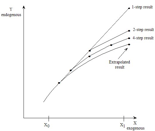
Figure 26.2 Two subintervals
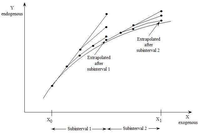
An Extrapolation Accuracy Summary (see section 26.2) is output to the terminal after each subinterval. If you are also creating an Extrapolation Accuracy file (see section 26.2.3), the results for the variables are output to it for each subinterval; these results are the endogenous movements just across the current subinterval.
For example, if you have 2 subintervals and a percentage-change variable X increases by 5 per cent across the first subinterval and by 4 per cent across the second one, this means it will increase by the combination of these, namely 9.2 per cent, across the whole simulation. The Solution file will show 9.2 while the Extrapolation Accuracy file will show 5 and 4 for the two subintervals.
When several subintervals are used (with or without user-specified accuracy), FORMULA(INITIAL)s are only carried out during the first step of the first subinterval. [Values in subsequent steps and subintervals are determined from these initial values taking into account UPDATE statements.]
26.3.1 Overall accuracy summary when more than one subinterval [gpd3.7.3.1]
If you use more than one subinterval, the LOG file contains an Extrapolation Accuracy Summary for the variables in each of the subintervals. However it is not easy to combine these to obtain an accuracy summary for the whole result.
An Overall Accuracy Summary is produced when the simulation uses two or more subintervals. This includes most simulations solved using automatic accuracy (section 26.4).
The Overall Accuracy Summary looks very similar to the Extrapolation Accuracy Summaries for each subinterval.
For example, suppose that there are just three subintervals. Consider a scalar variable with the following accuracy:
- accurate to 5 figures in the first subinterval with code FCX (Fair Confidence in eXtrapolated result)
- accurate to 3 figures in the second subinterval with code MC? (Monotonic, appears to be converging)
- accurate to 4 figures in the third subinterval with code OC? (Oscillating, appears to be converging)
Then the Overall Accuracy Summary will count this as being accurate to 3 figures (the lowest of the three) with code OC? (the worst of the three).
Note that taking the worst of the number of accuracy figures is a reasonable estimate provided that the number of subintervals is not too large. For example, suppose that, in every subinterval, the result for a scalar variable is accurate to 5 figures. If there are only 3-4 subintervals, you can be reasonably confident that the overall result for this scalar variable is still accurate to 5 figures. But if there are 100 subintervals, it is highly likely that the overall result would only be accurate to 3 or 4 figures.
26.4 Automatic accuracy for simulations [gpd3.7.4]
Automatic accuracy (sometimes called user-specified accuracy) has two motivations.
Firstly it allows you to specify the required accuracy needed in a simulation. You can specify this accuracy in advance and let the programs (GEMSIM or TABLO-generated programs) decide how many steps and how many subintervals to take to achieve the accuracy you have specified. See section 26.1.1 above for an example.
A second advantage is that, when used in conjunction with range restrictions in your TABLO Input file (see section 25.4), automatic accuracy ensures that the Coefficients never stray outside the specified range. See section 25.4.3 for an example of this.
This option is only available if you use a Command file. The simulation must be a multi-step one and it must be one in which you extrapolate from 3 separate multi-step calculations.
The statements in a Command file which let you specify the accuracy are shown below.
Automatic accuracy = yes|NO ; ! NO is the default accuracy figures = <d> ; ! 4 is the default accuracy percent = <pp> ; ! 80 (percent) is the default accuracy criterion = DATA|solution|both ;! data is the default
If you specify "automatic accuracy = yes ;" then the default is to require at least 80 percent of the extrapolated data results to be accurate to at least 4 figures. [See section 26.2.2 above for Extrapolation Accuracy Summaries for the (updated) data.]
When you ask for automatic accuracy, the software solves the simulation using several subintervals, and varies the length of the subintervals to achieve the required accuracy. You can give it a hint as to how many subintervals to try by including a statement in your Command file of the form
subintervals = <number> ; ! Default is 2 (for automatic accuracy)
For example, if you suggest 10 subintervals, the software will give one-tenth of the shocks as the first subinterval and then see if the required accuracy has been achieved over this subinterval. If so, it will go on to the next subinterval (and it may increase the length of the second subinterval). If not, it reduces the length of the subinterval and re-does this first subinterval. If you don't indicate how many subintervals in your Command file, the default is to begin with 2 subintervals.
You do not need to specify the number of steps to take across each subinterval. By default, the software carries out 2,4,6-step calculations (followed by extrapolation) in each subinterval. However, if you specify different numbers of steps (for example "steps = 1 2 4 ;" with Euler's method), this many steps will be used in each subinterval. As usual, Gragg's method is used by default unless you specify another method.
Although the software varies the length of the different subintervals, it always takes the same number of steps across each subinterval when giving user-specified accuracy.
Note that the accuracy you require is achieved for each subinterval, which is not exactly the same as requiring this accuracy across the whole simulation. The Overall Accuracy Summary (see section 26.3.1) gives the best indication of the overall accuracy of your results.
The accuracy criterion can be either data, solution or both. When it is data, the Extrapolation Accuracy Summary for all data files (see section 26.2.2 above) is used to decide if the required accuracy has been achieved. If it is the solution, the Extrapolation Accuracy Summary for the levels variables (see section 26.2.1 above) is used. If you specify "both", the total of these two summaries is used.
The default accuracy criterion is the data since this is somehow the intrinsic numerical information underpinning the model. If you use the solution as the accuracy criterion, the results can be affected by how many summary variables you attach or which variables' results are taken into account (see section 26.4.1 below).
We recommend that you experiment slowly with this procedure and that you do not specify very high accuracy until you have first tried lesser accuracy (for example, tried using the default accuracy of at least 80 percent accurate to at least 4 figures). The example in section 26.1.1 is relevant in this context.
If you are using automatic accuracy and the Left Hand Side Matrix is singular in one step of a subinterval, the subinterval is redone with a shorter length. This may work around a singularity along the path from the pre-simulation values of the exogenous values to the post-simulation values9.
26.4.1 Specifying which solutions to use [gpd3.7.4.1]
When the accuracy criterion is "solution" or "both", the solutions used in the accuracy test are the XAC-retained variables. This means that, if you wish to only take into account certain variables in the accuracy test at the end of each subinterval, you can achieve this by selecting just those variables as the XAC-retained ones (see section 26.2.6). For example, you may be happy with the results of a certain application provided all macro results and all export volume results are sufficiently accurate; in this case, select these to be the XAC-retained variables via a statement like .
xac-retained %macro p_exports ;
in your Command file (assuming that p_exports is the variable denoting percentage changes in export volumes).
Note that, even if you are not saving an Extrapolation Accuracy file (that is, you do not have the statement "extrapolation accuracy file = yes ;" in your Command file), you can still select a set of XAC-retained variables to be used as the accuracy criterion.
26.4.2 Incompatibilities [gpd3.7.4.2]
Note that "automatic accuracy = yes ;" is
- incompatible with option NUD (no final updates — see sections 25.1.8 and 33.1),
- incompatible with Newton's method (see section 26.6 below),
- incompatible with the SUP and SSL statements described in section 26.8.
26.4.3 Adaptive stepsize method [gpd3.7.4.4]
The method used to implement user-specified accuracy is simply a variant of the well-known "adaptive stepsize" method often used when solving differential equations [for example, Chapter 15 of Press et al. (1986)].
26.4.4 Stopping if subintervals become too small [gpd3.7.4.5]
It may happen that your simulation cannot be solved with the specified accuracy. [This may be because you have made an error with the model or in specifying the shocks. Or it may happen because you have specified greater accuracy than is appropriate.] Then the software will continue to reduce the subinterval length. You need some way of stopping the simulation so that it does not go on for ever.
For this reason, you can specify the minimum subinterval length allowed and you can say what happens if that minimum is reached. [Normally you would want the simulation to stop with an error if the minimum is reached.] The following Command file statements can be used.
Minimum subinterval length = * ; ! default is 0.000001 ( 10-6 )
for example,
minimum subinterval length = 0.000000001 ; minimum subinterval length = 1.0e-9 ;
[The minimum length can be specified in decimal (eg, 0.00001) or exponential (eg, 1.0E-9) notation.]
minimum subinterval fails = STOP|continue ; ! default is "stop"
If the current subinterval has the minimum allowed length and the accuracy criterion or range test still fails, this tells whether the simulation stops at this point or continues. If it continues, the subinterval length stays fixed at the minimum allowed subinterval length even though one or more range tests are failing. [Accordingly, continuing is not advised because your simulation results will be based on values out of the acceptable range.]
26.4.5 Controlling which values are tested [gpd3.7.4.6]
Ensuring that values of coefficients do not go outside the allowed range (as specified in the TABLO Input file — see section 25.4) is an important feature of automatic accuracy.
You can control which values (initial, updated, extrapolated) are tested and what happens if a value is out of range by using the Command file statements
range test updated values = updated|extrapolated|BOTH|no|warn ; range test initial values = YES|no|warn ;
When you are doing user-specified accuracy, the default values are BOTH and YES respectively10. To get the full benefits of user-specified accuracy, you must leave these at these default values.
For example, if the relevant "range test ..." is set at "WARN", a warning is shown for the first few instances out of range but the simulation carries on as if these warnings were not given. [In particular, the subinterval is not redone. So results may be based on values which are out of range.]
These range test statements can also be used when you are not doing user-specified accuracy - see section 25.4.4.
26.4.6 Checking progress during a run [gpd3.7.4.7]
If you are solving using user-specified accuracy, there may be several subintervals, and the run may take a long time. It can be difficult to tell from the screen output how far the simulation has progressed.
For this reason the program writes an additional file, the Automatic Accuracy Log file, which you can look at from time to time to check on the progress. This file has suffix .aal and the first part of its name is the same as that of the Solution file. [For example, if the Solution file is sjlb.sl4 then sjlb.aal is the name of the Automatic Accuracy Log file.] You can copy this file to some other file at any stage during the run and then examine its contents. However, do not edit this file since then, the program may not be able to update it at the end of the next subinterval which could cause the simulation to crash.
The Automatic Accuracy Log file has one line for each successfully completed subinterval. This shows how much of the simulation has been completed and when that subinterval was finished. A new line is added to the file at the end of each successful subinterval. For example, the file may contain the following lines:
Subinterval 1. Completed 25.000000 percent. 06:51:44 Subinterval 2. Completed 55.000000 percent. 06:52:30 Subinterval 3. Completed 91.000000 percent. 06:53:11 Subinterval 4. Completed 100.00000 percent. 06:54:02
The program also writes progress information to the screen (and log file) each time it begins the LU decomposition. This information looks like:
[Completed 13.3434 percent of whole sim. Subint 12 will do 10.5432.]
This tells you how much of the whole simulation has been completed before the start of the current subinterval. It also tells you how much more of the whole simulation will be completed if this subinterval is successful.
26.5 Runge-Kutta solution methods [rungekutta]
From GEMPACK Release 12.2 (2024), several new solution methods are available, drawn from the Runge-Kutta family of solution methods (see https://en.wikipedia.org/wiki/Runge-Kutta_methods).
Under suitable conditions the Runge-Kutta methods are likely to yield more accurate solutions for the same simulation time as the Euler, Midpoint or Gragg methods; or a faster solution with the same accuracy as the older methods.
You can specify Runge-Kutta in your CMF file as follows:
method = RungeKutta; RK flavor = RK4; ! Choose from RK2, RK4 (the default), BoSha32 or DoPri54 steps = 2; ! one number only, no extrapolation
Some details of the 'flavors' are listed in the table below.
| keyword | order | embedded order | passes | adaptive | literature name |
| RK2 | 2 | - | 2 | no | explicit midpoint |
| RK4 | 4 | - | 4 | no | classic fourth order |
| BoSha32 | 3 | 2 | 4 | yes | Bogacki-Shampine |
| DoPri54 | 5 | 4 | 7 | yes | Dormand-Prince |
Above, the 'passes' column shows how many calculations of equation coefficients and linear solves are needed for a single step. One RK4 step requires 4 such passes, and so might take as long as 4 Euler steps (For Euler, no. of steps = no. of passes). One DoPri54 step makes 7 passes, taking as long as 7 Euler steps.
Euler, Midpoint and Gragg methods allow you to calculate 3 solutions with increasing numbers of steps. The CMF might contain:
method = Euler; steps = 4 6 8;
GEMPACK extrapolates from these 3 solutions to create both a final, more accurate, solution, and an estimate of how accurate the solution is for each variable. However, the Runge-Kutta methods do NOT allow 3 solutions with extrapolation and so cannot estimate accuracy in this way.
However, the BoSha32 and DoPri54 are embedded methods which do provide estimates of accuracy. One DoPri54 step, for example, uses 7 function evaluations to calculate a fifth-order solution estimate and an estimate of the error of that solution.
26.5.0.1 The cumulative error estimate and the .acc file [errorestrk]
If you choose either of the BoSha32 or DoPri54 methods, estimated errors for each variable are written to the ≤sl4≥.acc file (where ≤sl4≥ is the basename of the solution file). For multistep simulations, the errors are accumulated.
The error estimates are reported in terms of the GEMPACK difference metric with formula:
ΔGP = Δcum / max(1.0,|Xcum|)
Above, Δcum is the cumulative difference between two solutions of different order, while Xcum is the cumulative solution.
For example, if the 5th-order estimate was 7% with error of 2,
the error metric would be |2|/max(1.0,7) = 2/7 = 0.286.
If the 5th-order estimate was 70% with error of 20,
the error metric would be |20|/max(1.0,70) = 20/70 = 0.286.
If the 5th-order estimate was 0.7% with error of 0.2,
the error metric would be |0.2|/max(1.0,0.7) = 0.2/1 = 0.2.
A face value, ranging from 1 (worst) to 10 (best), is written to the log file depending on the largest error estimate found in the simulation. The assignment is simply done in brackets of 0.02. E.g. a simulation with the worst error metric of 0.01 will get face value 10 as it falls in the bracket 0-0.02, whereas a error metric value of 0.11 would only be rated 5, as it falls in the bracket 0.1-0.12. This face value is used by RunDynam, WinGem and ViewHar when the accuracy of RK simulations is reported.
The .acc file has a numeric header for each variable. The variable name is stored in the coefficient name part of the header, but may be truncated to 12 characters. The full variable name appears in the long name (label part) of the header.
The simplest way to gather information from the .acc file is to set ViewHar (via the File->Options menu) to show the maximum values of real headers on the title page. In the GP12.2 version of ViewHar it is then possible to sort all headers by the maximum entry by a middle mouse button click on the Max column header. This shows at a glance the variables which are least converged. To allow this sorting to work, it is not possible to present the solution values in the same file. Instead it is possible to open the sl4 file in another ViewHar (SOL view mode) on the side. The header names of the .acc file resemble those used in the SOL view and thus allow for quick referencing between the two files.
26.5.0.2 Using the .acc file to track down problems [usingaccfile]
For simulations which are hard to solve accurately, the .acc file can give clues pointing to the source of the problem. For example, if large errors are associated with a particular sector, perhaps the initial data for that sector is strange, or contains zeroes which are not handled correctly.
If there is a problem with a particular equation, variables directly determined by that equation are likely to show larger errors. Typical problems in the tablo code might be:
- Missing linear variable for changing coefficients
- Incorrect linearization
- Non-differentiable adjustments to coefficients
Another potential cause is imbalances in the model database.
26.5.0.3 Large error metric from subtractive cancellation [largeaccval3]
Consider the following example: the levels equation C=A-B and the corresponding ordinary change form dC=dA-dB. Assuming dA and dB are of the order 106 and their associated errors are of order 10. In this case the error metric for dA and dB is of the order 10-5, which is close to the limit of the numeric accuracy achievable. However, if dA and dB are almost identical |dC| will be small (100 for this example). The error of dC is computed as the absolute sum of the error of dA and dB (10+10=20). Hence the error metric of dC becomes 0.2, which is orders of magnitude larger than the constituent errors.
One way to hide this problem is to substitute out dC from the equation system. Or it may be possible to rewrite the model in a way to avoid the issue.
26.5.1 Adaptive stepsize for Runge-Kutta [adaptiverk]
Euler, Midpoint and Gragg methods offer an automatic accuracy option which increases the number of steps (i.e., reduces stepsize) to achieve a specified level of accuracy. The BoSha32 and DoPri54 RK flavors offer a similar facility. You could specify this in your CMF file as follows:
method = RungeKutta; RK flavor = DoPri54; ! Choose from BoSha32 or DoPri54 steps = 2; adaptive step size = yes; ! no is the default epsTolerance = 0.1; ! 0.1 is recommended, lower for higher accuracy
Adaptive stepsize as implemented for Runge-Kutta resembles but differs in detail from the automatic accuracy used in conjunction with Richardson extrapolation. At each step error estimates are obtained for all variables. If any of the conditions below apply, the step is repeated with a smaller stepsize:
- The maximum (over all variables) error exceeds epsTolerance.
- Range tests on coefficients fail.
- One or more Assertions are untrue.
- A percent-change variable goes below -100 (changes sign).
Conversely, if none of the above apply the stepsize may be cautiously increased.
The default epsTolerance of 0.1 in most cases yields sufficiently accurate results. More accurate results can be obtained by lowering the value of epsTolerance. This might be required if the problem takes many steps to solve. This is because epsTolerance only controls the per-step error while the cumulative error includes contributions from all steps. However, we recommend not to use a value below 0.005 as numerical noise can become an issue and the simulation might fail to complete.
There are two more advanced CMF options, that are related to range check and assertion failures in combination when using adaptive stepsize.
retryAdjustmentFactor = 0.7 ! range 0-1, default 0.5 maxConsecutiveRetries = 5; ! default 3
The option retryAdjustmentFactor determines the stepsize reduction used when checks have failed. Values below 0.1 will increase the simulation time significantly. maxConsecutiveRetries controls after how many consecutive stepsize reductions the simulation will fail. Both options are connected in how they change the minimum stepsize upon encountering failed checks. That is, changing either retryAdjustmentFactor to 0.25 or maxConsecutiveRetries to 6 will each allow for a maximum stepsize reduction of 0.56. The difference is in the time it takes to reach the limit or the resulting stepsize if the simulation recovers.
26.5.2 Which RK integrator to choose? [whichrk]
For most purposes we recommend using one of the DoPri54 or BoSha32 embedded integrators as these provide .acc files which allow for insight into the quality of the solution. The drawback is the slightly higher cost incurred by having more stages than the explicit methods such as RK4. If the user is concerned about time to solution, e.g. in recursive dynamic models, it can be beneficial to only use the embedded methods in the shocked years and switch to RK4 in the remainder.
Generally we recommend using adaptive stepsize. With its capability to react to assertion and range check errors, it can avoid problems of Coefficients exceeding their bounds, which otherwise might only be achieved by using a large number of integration steps.
For simulations with large shocks, it can sometimes be more efficient to switch to the BoSha32 integrator. The reason is, that the accuracy is not the main factor causing step recomputations but variables exceeding their defined bounds due to small integration errors. In this case, the lower order integrator can be more time efficient as the number of steps required for an accurate solution will be similar but the cost per step is reduced.
26.6 Newton's method for levels models [gpd3.7.5]
Newton's method is sometimes an efficient way to solve levels equations. When a reasonable starting guess can be made for the solution of the levels equations, the method converges rapidly. However if the starting solution is not a good guess, there is no guarantee that the solution will converge at all.
Newton's method can be used in GEMPACK with levels models in certain circumstances. TABLO is used to add the appropriate Newton correction terms to linearised form of the levels equations. With this implementation of the model, GEMSIM or the TABLO-generated program can be used to run a simulation using the following ways of using the Newton terms:
The shock to the Newton variable can be added to the usual shocks in an Euler solution, and/or
the Newton shock can be applied alone in a series of Newton correction steps after a single or multistep Euler simulation.
The Newton variable is called $del_newton [TABLO introduces this name automatically]. For a levels equation
F = 0
the linearised equation, in terms of the change in F (written below as dF) and the Newton correction, is
dF = - F * $del_newton
For percentage change differentiation of the levels equation
F = G
the linearised equation, in terms of the percentage changes in F and G (written as pF and pG below) is
pF = pG - (1 - G/F) * 100 * $del_newton
-
To use TABLO to add this $del_newton term to all levels equations, choose option
NWT - Add Newton-correction terms to levels equations
from the main TABLO menu (the one presented before the CHECK stage — see section 9.1). - When you run GEMSIM or the TABLO-generated program (after compiling and linking as usual - see section 8.2), use Newton as the solution method.
- Set the variable $del_newton exogenous, but give no shocks to $del_newton.
- You need to specify whether the Newton correction is applied during and/or after each step in the multi-step simulation. You can choose to apply just the usual shocks with no Newton correction or the usual shocks and simultaneously a Newton correction. After each step you can apply none, one or several Newton corrections to improve the accuracy of the solution. There are Command file statements for doing this — see section 26.6.5.
Typical CMF options might be:
method = newton ; steps = 10 ; ! Number of Euler steps newton shock = yes; ! Add Newton correction to each Euler step newton steps-per-euler = 0 ; newton extra-steps-at-end = 5; report newton errors = all ; exogenous $del_Newton ;
As an example of Newton's method for the Levels model MOLV.TAB, run TABLO using the Stored-Input file MOLV-NWT.STI. The relevant files are supplied with the GEMPACK examples — see section 60.3. At the Command prompt, enter
tablo -sti molv-nwt.sti ltg molv-nwt
The Executable-image MOLV-NWT.EXE produced can be run using the Stored-input file MOLVNWT1.STI.
molv-nwt -sti molvnwt1.sti
This runs a simulation from the Command file MOLV-NWT.CMF using Newton's method.
26.6.1 Newton's method and ORANIF [gpd3.7.5.1]
In testing this method using a levels version of ORANIF, difficulties were encountered with zeros in the database and zero divides. Since the Newton-correction term is evaluated as part of an equation, you cannot use the ZERODIVIDE defaults available for formulas. In general it is possible to use IF syntax (see section 11.4.6) instead.
In the expressions for CES, CET and Cobb-Douglas functions, there are various expressions of the form A raised to the power B or involving the logarithm of A. In these expressions A must be positive, not zero. In practice this can be set up initially by setting levels variables which occur in CES, CET and Cobb-Douglas functions to at least "tiny", a small positive number. This was done even in cases where strictly speaking the levels variable would be identically zero eg if commodity c is not used at all in industry i. First the levels variable eg V1BAS was read in from a file, then a FORMULA(INITIAL) was used to change any values less than tiny.
FORMULA(initial) (all,c,COM)(all,s,SRC)(all,i,IND)
V1BAS(c,s,i) = V1BAS(c,s,i) +
IF(V1BAS(c,s,i) lt tiny, tiny - V1BAS(c,s,i));
Condensation
Condensation becomes more complicated due to the addition of the $del_newton terms to each equation. To overcome this the equations for CES functions were not substituted or backsolved, leading to a less condensed system of equations. The increase in solve time caused by the increased size of the Equations matrix was offset by the fact that Newton converges faster so fewer steps could be used.
Condensation also caused division-by-zero and invalid-exponentiation problems (see section 34.3) since the symbolic differentiation is not clever enough to cancel common factors in the numerator and denominator.
26.6.2 Convergence [gpd3.7.5.2]
When Newton converges, it does so rapidly - you can check convergence by checking the total of the Newton correction terms (that is, sum of the absolute values of the coefficients of $del_Newton) which is output to the terminal and/or LOG file after each Newton step. However if the starting solution is not reasonably close to the correct solution, there is no guarantee that the solution will converge at all. In fact it can go wildly wrong and end up in a region where the CES functions are not defined (eg negative prices), causing the program to crash with a Fortran error such as undefined exponentiation.
26.6.3 General advice [gpd3.7.5.3]
Extrapolation does not work with Newton's method.
In practice, a one-step or two-step Euler followed by 3 or 4 Newton steps gave good accuracy for various models. Solving ORANIF using a 1 step Euler followed by a 3 step Newton gave similar accuracy to 8,10,12 Gragg and extrapolation without Newton. The CPU time for the Euler-Newton was 44 secs which compares favourably with 48 secs for the fully linear version of ORANIF with 8,10,12 Gragg.
Newton's method can also be used to check the accuracy of the initial solution since the Newton terms at the first step are a calculation of the error in the equations for the original data. Information about the size of the Newton correction terms is given even if you are not doing a simulation.. (Put "simulation = no ;" and "nwt = yes ;" in your Command file to see this information.)
Adding homotopy terms to levels equations (see section 26.7) may be preferable to using Newton's method in some cases. There may be convergence using the adding homotopy terms method in cases where there would not be convergence using Newton's method starting from the same initial guesses.
Levels models are available for Stylized Johansen, Miniature ORANI and ORANIF (see chapter 42).
26.6.4 Newton's method is not reliable with mixed models [gpd3.7.5.4]
Note that we do not recommend Newton's method with any models except fully levels ones.
We do not recommend the use of Newton's method with mixed models (those whose TABLO Input files contain some levels and some linearised equations). In such a case, TABLO is only able to add the Newton correction terms to the levels equations. We have found that the solution appears to converge but that it can converge to the "wrong" solution in these cases (that is, to a solution which is not a solution of the underlying levels model).
26.6.5 Command file statements for Newton's method [gpd5.9.13]
Newton's method can be controlled using the following Command file statements:
method = newton ; newton shock = YES | no ; !optional, default = yes newton steps-per-euler = <d1> ; !optional, default <d1> = 2 newton extra-steps-at-end = <d2> ;!optional, default <d2> = 4
Examples
1: The simplest way is to just change the method to newton, and specify the number of (Euler) steps. (For example, see SJLVLBNW.CMF in section 26.6.5.2 below.)
method = newton ; steps = 4 ;
The simulation uses the default values so the actual steps are:
| 1 Euler step (with Newton correction added) then 2 Newton steps |
| 1 Euler step (with Newton correction added) then 2 Newton steps |
| 1 Euler step (with Newton correction added) then 2 Newton steps |
| 1 Euler step (with Newton correction added) then 6 Newton steps |
2: If you want to specify more closely the number of Newton steps you could use:
method = newton ; steps = 1 ; newton shock = no ; ! Do not add Newton correction to Euler steps newton steps-per-euler = 0 ; newton extra-steps-at-end = 3 ;
The simulation will do 1 ordinary Euler step (with no Newton correction included in the simulation shocks), then 4 Newton correction steps after it. (For example, see SJLVLBNW2.CMF in section 26.6.5.3 below.)
Command file statements for Newton's method are documented in section 26.6.5.1 below. We describe simple examples in sections 26.6.5.2 and 26.6.5.3 below.
26.6.5.1 Details of the Newton's method command file statements [gpd5.9.13.1]
method = newton ;
This is a new method which is an alternative to the usual methods Euler, midpoint, Gragg and Johansen. This statement sets the method to Newton's method.
When the method is set to Newton using "method = newton ;" no questions are asked during the separate steps of the simulation. The program either uses values from the other Newton Command file statements listed below, or if they are omitted, it uses the default values.
With "method = newton ;", the option NWT or Command file statement "NWT=yes;" is not allowed.
The simulation does several Euler steps as specified by the usual "steps = ...;" statement. You can only use a single multi-step solution, for example "steps = 5 ;" You can not use 2 or 3 multi-steps followed by extrapolation (as in "steps = 1 2 4 ; !wrong") because extrapolation does not work when you are using Newton's method. Within the program, the method used is really Euler and the "steps=.." command says how many Euler steps are to be used. The extra Newton steps are specified below or from the defaults.
newton shock = YES | no ; ! optional, default is "yes"
If you have "newton shock = yes ;" or this statement is omitted, the program will add a Newton shock (see section 26.6) to the variable $del_Newton when carrying out each of the Euler steps.
If you have "newton shock = no;", the usual shocks for Euler's method will be applied at each Euler step.
This statement can only be used in combination with "method=newton;".
newton steps-per-euler = <d1> ; ! optional, default <d1> = 2
The integer <d1> gives the number of Newton steps carried out after each Euler step. If this statement is not present after "method = newton ;" then the default value of <d1> = 2 is used.
This statement can only be used in combination with "method=newton;".
newton extra-steps-at-end = <d2> ; ! optional, default <d2> = 4
The integer <d2> gives the number of extra Newton steps carried out after the final Euler step, so that the number of Newton steps after the final Euler step will be <d1> + <d2>. If this statement is not present after "method = newton ;" then the default value of <d2> = 4 is used.
This statement can only be used in combination with "method=newton;".
26.6.5.2 Example: SJLVLBNW.CMF [gpd5.9.13.2]
In the GEMPACK examples, there are two Command files using Newton's method: SJLVLBNW.CMF and SJLVLBNW2.CMF.
The levels model used is SJLV using the TABLO-input file SJLV.TAB.
First run TABLO taking inputs from the Stored-input file SJLVNWGS.STI (which selects option NWT at the start and which produces output files for GEMSIM called SJLV-NWT.GSS and .SJLV-NWT.GST).
Then run GEMSIM taking inputs from the Command file SJLVLBNW.CMF (you will also need the file sj.har).
Notice that the Newton correction variable $del_Newton is declared as exogenous in these Command files.
In Command file SJLVLBNW.CMF, the default values of various Newton's command file statements are used. As in example 1 in section 26.6.5, the simulation carries out:
| 1 Euler step (with Newton correction added) then 2 Newton steps |
| 1 Euler step (with Newton correction added) then 2 Newton steps |
| 1 Euler step (with Newton correction added) then 2 Newton steps |
| 1 Euler step (with Newton correction added) then 6 Newton steps |
Part of command file SJLVLBNW.CMF
auxiliary files = sjlv-nwt ; ! Rel 9 command file statements for Newton's method method = newton ; steps = 4 ; ! Closure exogenous p_xfac ; ! for Newton's method $del_Newton must be exogenous exogenous $del_Newton ; rest endogenous ;
Have a look at the LOG file SJLVLBNW.LOG produced to see the different Euler and Newton steps.
26.6.5.3 Example: SJLVLBNW2.CMF [gpd5.9.13.3]
In the Command file SJLVLBNW2.CMF, the simulation will carry out a 4-step Euler calculation (with no Newton's corrections). Then following the 4-step Euler, Newton's method is used to increase the accuracy of the simulation by applying the 3 extra Newton steps at the end.
Part of command file SJLVLBNW2.CMF
! Auxiliary files for model SJLV-NWT (from SJLV.TAB) ! In TABLO, choose option NWT auxiliary files = sjlv-nwt ; ! Rel 9 command file statements for Newton's method method = newton ; steps = 4 ; ! carry out 4 step Euler with no Newton corrections, then ! 3 extra steps at the end where the only shock is Newton correction newton shock = no ; ! the default is yes newton steps-per-euler = 0 ; ! default is 2 newton extra-steps-at-end = 3 ; ! default is 4 report newton errors = all ; ! default is initial ! Closure exogenous p_xfac ; ! for Newton's method $del_Newton must be exogenous exogenous $del_Newton ; rest endogenous ;
First run GEMSIM taking inputs from the Command file SJLVLBNW2.CMF.
Then look at the LOG file SJLVLBNW2.LOG to see where the Euler and Newton steps are done.
The statement
report newton errors = all ;
(see section 9.3) in the Command file asks the program to report information about the Newton errors after each Euler and Newton step.
Look at the log file SJLVLBNW2.LOG to see what is happening to the errors as the simulation progresses. (Search for "del_Newton".) You can see the Newton error terms are initially zero, then they increase during the Euler steps. After the fourth Euler step and before the first Newton step at the end, the
Sum of absolute values of the del_Newton terms is 0.479.
During the 3 subsequent Newton steps, the errors decrease to very small values:
Sum of absolute values of the del_Newton terms is 2.5629 E-04 Sum of absolute values of the del_Newton terms is 6.5565 E-05 Sum of absolute values of the del_Newton terms is 1.5497 E-04.
26.7 Homotopy methods and levels equations [gpd3.7.6]
If you have levels equations for which the natural data is not a solution, you can ask the TABLO to add homotopy terms. This can make it relatively easy to obtain results which are a solution to these levels equations.
You can ask TABLO to automatically add HOMOTOPY terms to all or selected levels equations — see section 26.7.5 for the syntax. HOMOTOPY is a reserved word (see section 11.2.1).
- Homotopy methods can assist in obtaining solutions to levels equations for which the natural data is not a solution. For example, this can be used to produce (eg, from data for one year) a non-steady state intertemporal data base which satisfies all the equations of the model, including the intertemporal ones (which probably would not be satisfied if the data for this one year is replicated to all years). Section 16.6.1 gives an example of this technique.
- Homotopy methods can be used to find (based on an initial guess which is not a solution) an accurate solution to a system of levels equations.
We give further examples below which illustrate these points.
The methods described here and automated by TABLO are methods introduced to the CoPS/IMPACT group of modellers by Mark Horridge. They have their origins in the so-called homotopy methods of mathematics (see, for example, the survey article by Watson (1986)) which can be used in various branches of science and engineering. In particular these methods are now an integral part of the MONASH (and other related) models [Dixon and Rimmer (2002)]. These methods are very powerful, as the examples below indicate.
Unlike Newton's method (see section 26.6), this methodology will work when only some of the equations of the model are written as levels equations in the TAB file. [There may also be many linear equations written in the TAB file.] Also, even if all Equations are Levels Equations, the solution may converge using the adding Homotopy terms method in cases where it would not converge using Newton's method starting from the same initial guesses.
26.7.1 Example 1 - solving a system of levels equations [gpd3.7.6.1]
Consider the two levels equations
Y = X + a
X2 + Y2 = 5
where "a" is a constant (that is, a parameter) and X,Y are the unknowns. We show how adding HOMOTOPY terms to (one of) the levels equations makes it easy to obtain accurate solutions of this system of (levels) equations. A suitable TAB file is shown below.
! Set defaults for Levels model ! EQUATION(DEFAULT=LEVELS) ; VARIABLE(DEFAULT=LEVELS) ; FORMULA(DEFAULT=INITIAL) ; COEFFICIENT(DEFAULT=PARAMETER) ; VARIABLE(DEFAULT=CHANGE) ; Set COM (c1-c3) ; Variable (all,c,COM) V1(c) ; Variable (all,c,COM) V2(c) ; Coefficient (parameter) (all,c,COM) coeff1(c) ; Formula (Initial) (all,c,COM) coeff1(c) = $POS(c) ; Formula (Initial) (all,c,COM) V1(c)= $POS(c)+2 ; Formula & Equation eq1 (all,c,COM) V2(c) = V1(c) + coeff1(c) ; Equation (ADD_HOMOTOPY) eq2 (all,c,COM) V1(c)^2 + V2(c)^2 = 5 ;
Here the single system of two equations above has been replaced by three different systems (one for each "c" in the set COM). The parameter "a" has been replaced by "coeff1(c)". The unknowns X and Y have been replaced by V1(c) and V2(c) respectively. Note that we have included the statement
Variable(Default=Change)
to make all associated linear variables into ordinary (rather than percent) change variables. This is because the variables in this example could be positive, negative or zero.
The assignment of initial (that is, pre-simulation) values to the variables is important and interesting. Here we have assigned essentially arbitrary initial values for V1(c) [V1(c)=$POS(c)+2]. Then those for V2(c) are naturally given by the Formula & Equation eq1 (which makes this equation satisfied by these initial values). Of course it is highly likely that the second equation eq2 will NOT be satisfied by these initial values.
This is why we have asked TABLO to add the HOMOTOPY terms to this equation eq2 via the "(ADD_HOMOTOPY)" qualifier in that equation. TABLO adds a term
CX(c)*HOMOTOPY
to the right-hand side of the equation11. Here HOMOTOPY is a Variable(Levels,Change) whose initial value is -1 and CX(c) is a Coefficient(Parameter) whose value is calculated so as to make the equation satisfied with the given initial values for V1(c) and V2(c). [Consider the "c1" equation. The initial values of V1 and V2 are V1("c1")=3 and V2("c1)=V1("c1")+COEFF1("c1")=3+1=4. Thus the LHS of eq2 is equal to 32 + 42 = 25 while the RHS is equal to 5+CX("c1")*(-1) since the initial value of HOMOTOPY is -1. Thus the initial value of CX("c1") must be -20 to make the two sides equal.]
To solve these equations, we carry out a simulation in which only the HOMOTOPY variable is shocked (by 1, from its initial value of -1 to its final value of 0). Notice that when HOMOTOPY has the value zero, the original equation eq2 (without the CX(c)+HOMOTOPY term) is satisfied. This is why the post-simulation values of the endogenous variables V1(c) and V2(c) are solutions of the two equations in question.
If you carry out the simulation you will find that the linear results are c_V1("c1")=c_V2("c2")=-2. This means that the solution to the "c1" versions of the equations is V1("c1)=1 and V2("c2")=2 (since the c_V simulation values are changes from the initial values of 3 and 4 respectively).
This is a simple example showing how adding HOMOTOPY terms to selected levels equations can make it easy to use GEMPACK to find solutions of a system of levels equations (starting from an initial guess - namely the pre-simulation values assigned by the READ and FORMULA(INITIAL) statements).
Note that HOMOTOPY terms only need to be added to selected equations. Note also that, in the example above, the other equation eq1 could have been included as a linearized equation in the TAB file without affecting the procedure.
You can find a similar example in section 26.9.2. There the HOMOTOPY terms are added explicitly in the TAB file. That section contains an explanation as to why the solution obtained satisfies the original levels equations.
26.7.2 Example 2 - finding an intertemporal data set [gpd3.7.6.2]
A data base for an intertemporal model consists of an input-output table for each year represented in the model. Since the model typically goes out into the future, input-output tables for these years are not available and have to be made up. Often this is done by taking the most recently available input-output table (say for the year 2000) and then replicating it for the other years (into the future). The problem is that the resulting intertemporal data set is almost certainly not a solution to the levels equations of the model. It will provide a solution to the "intra-period" equations (those involving just a single time instant) but will almost certainly not be a solution to the "inter-period" equations (those involving two or more time instants).
Of course it is important to be able to obtain an intertemporal data set which provides a solution of all the equations (including the inter-period equations) since a simulation in GEMPACK must start from such a solution. [GEMPACK simulations move from one solution to another. They produce unreliable results if they do not start from such an initial solution — see section 26.9 for more details.]
This problem of finding an intertemporal data set is a well known (and serious) problem for modellers building and solving intertemporal models using GEMPACK (see, for example, Codsi et al. (1992) and Wendner (1999)).
Adding Homotopy terms to the inter-period equations and then carrying out a simulation in which the Homotopy variable is shocked can solve this problem for many intertemporal models. See section 16.6 for more details and a detailed worked example.
26.7.3 Example 3 - use when adding behaviour to a model [gpd3.7.6.3]
Sometimes when you add behaviour to a model, there is not an obvious solution of the underlying levels equations you wish to add. For example, this happens in several parts of the MONASH model [Dixon and Rimmer (2002)]. Explicit homotopy terms were added to a few equations to get around the fact that the pre-simulation data does not give an initial solution. In MONASH.TAB [see chapter 4 of Dixon and Rimmer (2001)], the linearized homotopy variable is called del_unity. Examples of equations using del_unity include E_del_f_ac_p_y, E_d_f_fea_t_j, E_d_f_fcfc_t.
Considerable technical skill is required to add the correct homotopy terms in these cases by hand. Now it is easy since you can ask TABLO to do it for you. All you have to do is to
- add the relevant equation as a levels equation,
- tell TABLO to add the appropriate HOMOTOPY terms by including the qualifier "(ADD_HOMOTOPY)" when you declare the equation.
Of course adding levels equations does require a little technical skill. Help is available in the document Harrison and Pearson (2002). The relevant equations are naturally levels equations so inserting them as such in the TAB file is a sensible thing to do.
If you choose this route, you just need to remember to shock the linear variable c_HOMOTOPY by one in simulations.
Example from MONASH
The equation E_del_f_ac_p_y adjusts the quantity of capital from the pre-simulation value QCAPATT read in from the database to the new value QCAPPLUS1_B which is the quantity of capital after subtracting the depreciation and adding in the investment.
Formula(initial) (all,j,IND) QCAPPLUS1_B(j)=QCAPATT(j)*(1 - DEP(j)) + QINVEST(j)
The natural levels equation, which sets QCAPATT equal to the parameter QCAPPLUS1_B, is
Equation(Levels) E_del_f_ac_p_y (All,j,IND) QCAPATT(j) = QCAPPLUS1_B(j) + F_AC_P_Y(j) ;
where F_AC_P_Y(j) is a shifter which is initially equal to zero. (It is used to turn the equation off if we do not wish to use the equation.)
However this levels equation is not satisfied initially since QCAPATT on the data base is not equal to QCAPPLUS1_B. [The value of QINVEST(j) is effectively also read from the data base. The pre-simulation values of QCAPATT and QCAPPLUS1_B are only equal in the unlikely case that investment QINVEST in the pervious year exactly offsets depreciation.]
Below we show how this equation E_del_f_ac_p_y could be added to MONASH.TAB as a levels equation with the ADD_HOMOTOPY qualifier. The equation is:
Equation(Levels, ADD_HOMOTOPY) E_del_f_ac_p_y (All,j,IND) QCAPATT(j) = QCAPPLUS1_B(j) + F_AC_P_Y(j) ;
In order to obey the rules for levels equations, terms in this equation must be either levels variables or Coefficient(Parameter)s — see section 10.9. QCAPATT needs to be declared as a levels variable with associated linear variable cap_at_t, and QCAPPLUS1_B needs to be declared as a Coefficient(Parameter).
Variable(levels, linear_name=cap_at_t) (All,j,IND) QCAPATT(j) # Quantity of capital stocks, start of forecast year, ie K(t) Fq#; Coefficient(Parameter) (All,j,IND) QCAPPLUS1_B(j) # Qty of cap stock, end of data year, base FIq#; Formula(Initial) (All,j,IND) QCAPATT(j) = VCAP_AT_T(j)/PCAP_AT_T(j); ![[!Variable (All,j,IND) cap_at_t(j) # Capital stock at t (start of forecast year) #; !]]!
[See sections 10.4 and 9.2.2 for information about the Variable qualifiers "linear_name=" used above and "linear_var=" used a couple of lines below.]
We need to introduce the levels variable associated with the linear variable del_f_ac_p_y and set it initially to zero.
Variable(levels,linear_var=del_f_ac_p_y)(All,j,IND) F_AC_P_Y(j); Formula(initial) (all,j,IND) F_AC_P_Y(j) = 0.0 ;
When the homotopy equation is linearized, it is replaced by
Formula(Initial) !for new Coefficient(Parameter) CHOMO1@H!
(All,j,IND) CHOMO1@H(j) = QCAPATT(j) - {QCAPPLUS1_B(j) + F_AC_P_Y(j)} ;
Equation(linear) E_del_f_ac_p_y (all,j,IND)
QCAPATT(j)/100.0 * cap_at_t(j)=del_f_ac_p_y(j) - CHOMO1@H(j)*c_HOMOTOPY;
The coefficient of c_HOMOTOPY gives the homotopy correction term which is calculated in terms of initial or base values as
[QCAPATT(j) - {QCAPPLUS1_B(j) + F_AC_P_Y(j)} ]
The original equation in the MONASH.TAB in Dixon and Rimmer (2001) is the linear equation:
Equation E_del_f_ac_p_y
# Gives shock in yr-to-yr forecasting to capital at beginning of year t #
(All,j,IND) [QCAPATT(j) + TINY]*cap_at_t(j)
= 100*{QINV_BASE(j) - DEP(j)*QCAPATT_B(j)}*del_unity + 100*del_f_ac_p_y(j);
However since
[QINV_BASE(j) - DEP(j)*QCAPATT_B(j)}] = - QCAPATT(j) + QCAPPLUS1_B(j)
and F_AC_P_Y(j)} is initially zero, the term for the variable del_unity in the original equation in MONASH.TAB is the same as the term for c_HOMOTOPY so that the linearized homotopy equation is the same as the original equation in MONASH.TAB.
In order to run a simulation with the levels version of this equation, you would need to add the variable c_HOMOTOPY to the exogenous list and shock it by 1. Add to your Command file the statements:
exogenous c_homotopy ; shock c_HOMOTOPY= 1.0;
26.7.4 Formal documentation about ADD_HOMOTOPY [gpd3.7.6.4]
Here we describe in more formal terms what TABLO does whenever the qualifier "(ADD_HOMOTOPY)" occurs in a levels equation.
We illustrate this with the example equation:
Equation (Levels, Add_Homotopy) EQ1 (all,c,COM) X1(c) = A*X2(c) ;
where X1 and X2 are levels variables and A is a parameter. With this equation, TABLO will
- add a new Coefficient(Parameter) (All,c,COM) EQ1@H(c) [the name is based on the Equation name EQ1],
- give EQ1@H initial values via the Formula(Initial) (all,c,COM) EQ1@H(c) = X1(c) - A*X2(c),
-
add the term -EQ1@H*HOMOTOPY to the RHS of equation EQ1 so that it reads
(All,c,COM) X1(c) = A*X2(c) - EQ1@H(c)*HOMOTOPY, - linearize this modified equation in the usual way.
In general, TABLO
-- adds a new Coefficient(Parameter) whose name has "@H" added to the name of the equation,
-- adds a Formula(Initial) for this Coefficient, and
-- adds the term -<coef>*HOMOTOPY to the RHS of the levels equation12.
The linearized equation is shown on the INF (Information) file in the usual way (see section 18.3). Just above it on the INF file you will see the Formula(Initial) and the name of the new Coefficient. In the example above, you will see the following on the INF file:
! FORMULA(INITIAL) for new Coefficient(Parameter) EQ1@H
(ALL,c,com) EQ1@H(c) = x1(c) - {A * x2(c)} ; !
! Add term -EQ1@H*HOMOTOPY to RHS of levels eq EQ1 !
! EQUATION(LINEAR) EQ1
(ALL,c,com) x1(c) * p_x1(c) = A * x2(c) * p_x2(c)
- EQ1@H(c) * 100.0 * c_HOMOTOPY ; ! .
The levels variable is always called HOMOTOPY. It is always a (Levels,Change) variable whose initial value is set to -1. You should always shock its associated linear variable c_HOMOTOPY by 1 (which takes HOMOTOPY from -1 to 0)13.
The Coefficient added is a perfectly normal Coefficient. For example you can look at its values via xwrite statements (even WRITE statements after the equation in the TAB file) and in AnalyseGE.
26.7.5 Names for homotopy variables added to levels equations [gpd5.8.6]
You can ask TABLO to add Homotopy variables to some or all Levels Equations using the ADD_HOMOTOPY qualifier in Equation or Default statements. ADD_HOMOTOPY can only be added to a levels equation statement. Where the equation DEFAULT=ADD_HOMOTOPY is in force it is applied only to levels equations and is ignored for linear equations. You can see examples using this qualifier in section 16.6 and section 26.7. See also sections 26.7.4 and 26.7.6 for documentation about this qualifier.
Unless you specify otherwise (see below), the same Homotopy variable is added to all relevant equations, and the Homotopy Levels variable is always called HOMOTOPY.
However, you can choose a different name for these Levels Homotopy variables and you can use different names for different equations if you wish to [this would allow you to use subtotals solutions (see chapter 29) to show the effects of the different homotopy variables].
1: You can use the default statement
Equation (Default=ADD_HOMOTOPY=<default-homotopy-name>) ;
to set up the default name <default-homotopy-name> to be used for the homotopy levels variable to be added to any levels equations which follow. The Release 8.0 statement
Equation (Default=ADD_HOMOTOPY) ;
(which is still allowed without "=" after ADD_HOMOTOPY) is equivalent to
Equation (Default=ADD_HOMOTOPY=HOMOTOPY) ;
2: You can use the Equation qualifier
ADD_HOMOTOPY=<homotopy-variable-name>
to specify the name of the Levels Homotopy variable to be added to any levels Equation. The Release 8.0 qualifier ADD_HOMOTOPY (which is still allowed without a following "=") is equivalent to the qualifier ADD_HOMOTOPY=HOMOTOPY.
When TABLO comes to a levels equation,
- if there is an ADD_HOMOTOPY or ADD_HOMOTOPY=<name> qualifier in the statement the appropriate name is used for the levels homotopy variable added to the linearised equation.
- if a Default=Add_Homotopy statement is in force, and there is no ADD_HOMOTOPY or ADD_HOMOTOPY=<name> qualifier on the equation, the name specified in the Default statement is used for the levels homotopy variable added to the linearised equation.
The homotopy variable is always a levels variable. The associated linear variable always represents the change in that levels variable and the name of the associated linear variable always has c_ added to the start of the levels name.
The default statement
Equation (Default=NOT_ADD_HOMOTOPY) ;
cancels any default name set up (as well as cancelling the adding of a homotopy variable to following equations).
You must add the relevant homotopy variables to the exogenous list in your Command file (you can use either the levels name or the associated linear name) and you must give them all a shock of size 1.
ADD_HOMOTOPY example
Equation (Default=ADD_HOMOTOPY=homo1) ; Equation (Levels) eq1 <etc> ; Equation (Levels, Add_Homotopy=homo2) eq2 <etc> ; Equation (Default=NOT_ADD_HOMOTOPY) ; Equation (Levels, Add_Homotopy) eq3 <etc> ; Equation (Levels) eq4 <etc> ;
Above, the levels homotopy variables added are:
- homo1 to eq1,
- homo2 to eq2,
- HOMOTOPY to eq3.
No homotopy variable is added to eq4.
When you carry out a simulation, you should add homo1, homo2 and HOMOTOPY to the exogenous list and you should give each of these three variables a shock equal to 1.
26.7.6 ADD_HOMOTOPY and NOT_ADD_HOMOTOPY default statements [gpd3.7.6.5]
Any Levels Equation can be given one of these qualifiers ADD_HOMOTOPY or NOT_ADD_HOMOTOPY14. If so this tells TABLO whether or not to add Homotopy terms to this equation.
There are also DEFAULT statements (see section 10.19)
EQUATION ( DEFAULT = ADD_HOMOTOPY) ; EQUATION ( DEFAULT = NOT_ADD_HOMOTOPY) ;
which you can place anywhere in a TABLO Input file. After the first of these Default statements, Homotopy terms will be added to all Levels Equations encountered (unless the Equation has its own ADD_HOMOTOPY or NOT_ADD_HOMOTOPY qualifier). After the second of these Default statements, Homotopy terms are not added. You can use these Default statements to turn on or off the adding of Homotopy terms to groups of Levels Equations in your TAB file. These Default statements have no effect on Linear Equations.
26.8 Options for saving solution and updated data files [gpd3.7.7]
26.8.1 Saving solutions or updated data after each multi-step calculation [gpd3.7.7.1]
When you carry out two or three separate multi-step calculations and then extrapolate from them, you normally do not see the solutions or the updated data after each separate multi-step calculation — you just see the extrapolated solution and the data updated using that solution.
However, there are Command file statements to save the solution and/or the updated data after each multi-step solution.
You can use the following statements in your Command file to save one or all of these solutions.
SSL = all ; ! to save all multi-step solutions on the solution file SSL = last ; ! to save the last multi-step solution SSL = none ; ! to save just the cumulative solution - the default.
These extra solutions are saved as "subtotals" which you can view using ViewSOL.
For example, if you were running 1, 2, 4 Euler solution for your simulation, and you add to your CMF:
SSL = all ;
the three separate solutions corresponding to a 1-step Euler, a 2-step Euler and a 4-step Euler will be written on the Solution file as well as the extrapolated solution calculated from these three separate solutions.
For SSL= last ; you would just save the 4-step Euler and the extrapolated solutions.
To save the updated data files, after the two or three multi-step solutions, the syntax is similar:
SUP = all ; ! to save the updated data after each multi-step SUP = last ; ! to save after the last multi-step SUP = none ; ! the default.
The file names have the same file stem but use suffixes .UD5,.UD6,.UD7 (cf. section 22.5). For option SUP, the data files should be Header Array files. For original data files which are text files, the UD5, UD6 and UD7 files are saved in Header Array format (which can be looked at using ViewHAR or SEEHAR).
Neither of these options can be used if you have more than one subinterval (see section 26.3 above) or with user-specified accuracy (see section 26.4 above).
26.8.1.1 SSL and subtotals [gpd5.9.18]
If you have
- subtotal statements in your Command file and
- an SSL (save Separate multi-step SoLutions — see above - these solutions are saved as subtotal solutions) statement in your Command file,
the genuine subtotals (corresponding to the subtotal statements in your Command file) are the first subtotals put on the Solution file and the SSL solution(s) are the last subtotal(s) put on the Solution file.
For example, if your Command file contains the statements
method = euler ;
steps = 2 4 6 ;
ssl = last ;
subtotal p_XFAC("labor") = labor effects ;
then there will be two subtotals results on the Solution file. The first is the "labor effects" subtotal and the second is the SSL solution which is the 6-step Euler solution. [The subtotal description for this will be "Results from the 6-step solution".]
26.8.2 Saving updated values from all FORMULA(INITIAL)s [gpd3.7.7.2]
It is possible to ask GEMSIM or a TABLO-generated program to save updated values of all coefficients whose initial values are set via FORMULA(INITIAL)s. To do this, put statements
sui = yes ; updated formula initial data = <filename> ;
in your Command file. Then updated values of all coefficients (or parts of coefficients) whose initial values are set via a FORMULA(INITIAL) which does not have "WRITE UPDATED VALUE .." (see section 11.12.8) in it will be written to this file. The file containing these updated values is a Header Array file.
Example
If you add the following statements to the Command file SJLB.CMF (see Figure 3.8.1)
sui = yes ; updated formula initial data = sjlbfi.upd ;
the updated data file SJLBFI.UPD will contain the post-simulation values of prices and quantities initialised via FORMULA(INITIAL)s in SJ.TAB.
26.9 Solutions report perturbations of the initial values [gpd3.7.8]
When you solve a model using GEMPACK, the results reported (percentage changes or changes) are perturbations from the original values of the underlying levels variables. In particular, if the pre-simulation values of the Coefficients corresponding to the levels variables do not satisfy the levels equations of the model, the implied post-simulation values will not satisfy the equations. We give examples to illustrate this important point. In section 26.9.2 below, we show how the introduction of Homotopy terms (see section 26.7) can be used to produce post-simulation values which do satisfy the desired levels equations (even when the pre-simulation values do not).
Example 1.
Consider the very simple model with just one levels equation
| (E1.1) | X = 2Y |
The natural linearized equation to use is
| (E1.2) | p_X = p_Y |
which is obtained from the Product rule (see chapter 18) since 2 is a constant.
Suppose that you start a simulation from a point where X=1 and Y=1. Of course this is not a solution of the underlying levels equation (E1.1). If, say, Y is exogenous and is shocked by 10 percent, clearly from (E1.2) the simulation result for p_X will also be 10 percent. This would suggest that the post-simulation point is given by X=1.1 (10 percent more than 1) and Y=1.1. This point is not a solution of the underlying levels equation (E1.1) either.
Alternatively, you could use the Change Differentiation form
| (E1.3) | c_X = 2*c_Y |
Or, equivalently,
| (E1.4) | X*p_X = 2*Y*p_Y |
A TAB file for this, starting from X=1=Y is as follows.
Variable p_X ; Variable p_Y ; Coefficient X ; Coefficient Y ; Formula (Initial) X = 1 ; Formula (Initial) Y = 1 ; Update X = p_X ; Update Y = p_Y ; Equation eq1 X*p_X = 2*Y*p_Y ;
If you solve this (say Gragg 2,4,6) giving a 10 percent shock to Y, you would find that the result for p_X is 20. This would suggest the post-simulation point X=1.2 (20 percent more than 1), Y=1.1.
Why do these two linearizations give such different results? There are several things to consider.
- Firstly, since the starting point in each case (X=Y=1) does not satisfy the underlying levels equation (E1.1), there is nothing in the theory underpinning the GEMPACK solution methods to suggest that you should end up at a solution.
- Secondly, note that the derivation of the Product Rule (see the Example in section 18.2.1) specifically relies on the fact that the simulation starts from a solution to the underlying levels equation (since R=CPQ is substituted into the equation (9) there which is obtained by Change differentiation). Thus a the linearization (E1.2) is particularly inappropriate when the starting point is not a solution of the underlying levels equation.
- Thirdly, note that the derivation of the Change Differentiation rules (see section 18.2.1) does not appear to rely on substituting back the original levels equation. Thus the use of the change linearized form (E1.4) above does not seem to be quite so suspect. We elaborate on this point in section 26.9.1 below.
26.9.1 Change differentiation keeps a constant error [gpd3.7.8.1]
It turns out that, if you only use Change Differentiation (that is, avoid the use of any Percentage-change rules — see section 18.2.2), the "solution" that GEMPACK reports has the same error in the underlying levels equations as at the initial point.
To see what we mean by the "same error" consider again Example 1 above and consider the results based on the Change differentiation version (E1.4). The starting point is X=Y=1. The error in the underlying levels equation (E1.1) is RHS-LHS=2-1=1. The "solution" gives X=1.2, Y=1.1. The error at this point is
RHS - LHS = 2*1.1 - 1.2 = 1 .
Hence the error is the same.
This illustrates the general point that
If only Change Differentiation is used, the difference between the post-simulation LHS and RHS values is the same as that between their pre-simulation values.
In particular, when the pre-simulation values satisfy the underlying levels equations, so do the implied post-simulation levels values (since the difference is zero in both cases).
To understand the general point highlighted above, recall that GEMPACK uses only the linearized equations when it solves the model. But the linearized equations are no different if we add a constant to the either side of any of the levels equations. If, in Example 1 above, we had been thinking of the levels equation
| (E1.5) | X + 1 = 2Y |
(instead of X=2Y), this equation would be satisfied by the pre-simulation values X=1,Y=1. The Change Differentiation of this equation (E1.5) is the same as (E1.4). This levels equation (E1.5) is also satisfied by the implied post-simulation values X=1.2,Y=1.1.
Because GEMPACK only uses the linearized equations, when it solves the model it is in some sense integrating these linearized equations. As you know from elementary calculus, integration only determines the result up to an arbitrary constant15. Extra information is needed to determine that constant. In the GEMPACK case, this constant is the difference between the LHS and RHS when the pre-simulation values of the relevant Coefficients are substituted into the levels equation.
We give a second, less trivial example of what happens if the starting point does not satisfy the underlying levels equation and where only Change Differentiation is used.
Example 2.
Consider the model with just one levels equation
| (E2.1) | X2 + Y2 = 3XY |
The TAB file is shown below.
Variable (Levels) X ; Variable (Levels) Y ; Formula (Initial) X = 2 ; Formula (Initial) Y = 1 ; Equation (Levels) eq1 X^2 + Y^2 = 3*X*Y ;
The pre-simulation levels values X=2,Y=1 do NOT satisfy the equation (since the LHS=5 and the RHS=6).
Suppose that you solve this model, taking Y as exogenous and X as endogenous, and give a shock so that Y goes from its pre-simulation value of 1 to a post-simulation value of 1.6. The simulation results (using Gragg 20,30,40 steps to get accurate results) show a percentage change of 94.1619 for X. This increases X from 2 to 3.88324.
Do the post-simulation values of X and Y satisfy the levels equation eq1? The answer is clearly NO since the LHS=17.63955 while the RHS=18.63955. The RHS is still 1 more than the LHS (as it was with the pre-simulation values)..Note, however, that the error (difference between RHS and LHS values) is the same at the post-simulation point as it is at the pre-simulation point. This a further example of the general point highlighted above16 [TABLO uses Change differentiation when differentiating equation (E2.1) because of the + sign on the LHS — see section 9.2.5.17 ]
26.9.2 How can homotopies help? [gpd3.7.8.2]
Suppose that you have a levels equation you wish to include in your model but that you cannot easily obtain pre-simulation values of the relevant Coefficients which satisfy this equation. That might be the case for the equation (E2.1) in the example above. It is certainly the case in recursive dynamic models and intertemporal models for the capital accumulation equation if investment in the single year data base you are starting from is more or less than that required just to offset capital depreciation. [See section 26.7 above and section 16.6.]
Homotopy methods are described in section 26.7. Introducing a Homotopy variable (this is a levels variable) and giving it a suitable pre-simulation value is a cunning way of ensuring that the post-simulation values do satisfy the desired levels equation, even though the pre-simulation values may not satisfy the equation.
The previous sentence may seem mysterious to you, and possibly it seems to contradict what we said in the section above. We explain more below.
Consider again the equation
| (E2.1) | X2 + Y2 = 3XY |
from Example 2 in section 26.9.1 above. Suppose that this is the equation we wish to include in our model. Suppose, as in the example above, we start with pre-simulation values X=2,Y=1. [These do not satisfy the equation.] How can we achieve post-simulation values which satisfy this equation? The secret is to modify the equation in the TAB file by adding a suitable Homotopy term. The modified equation is
X2 + Y2 = 3XY + C*HOMOTOPY
where HOMOTOPY is a levels, change variable, and C is a suitable constant.
Suppose that we take the pre-simulation levels value of HOMOTOPY to be -1 and choose the value of C so that this modified equation is satisfied with these pre-simulation values, namely
X=2, Y=1, HOMOTOPY= -1.
Clearly we need C=1. Thus the modified equation is
| (E2.2) | X2 + Y2 = 3XY + HOMOTOPY |
Now, when we solve the model, as well as shocking Y by 60 percent, we shock HOMOTOPY from its pre-simulation value of -1 to a post-simulation value of 0 (that is, give a shock of +1 to c_HOMOTOPY). Since the pre-simulation values (of X,Y,HOMOTOPY) satisfy the levels equation (E2.2), so will the post-simulation values. But the post-simulation value of HOMOTOPY is zero. Hence the post-simulation values for X and Y must satisfy the original equation (E2.1).
If you carry out this simulation after modifying the TAB file from the section above to include the statements18 :
Variable (Levels, Change) HOMOTOPY2 ; Formula (Initial) HOMOTOPY2 = -1 ; Equation (Levels) eq1 X^2 + Y^2 = 3*X*Y + HOMOTOPY2 ;
you will find that the simulation result for p_X is 109.4425 which means that the post-simulation levels value of X is 4.1888519. Note that X=4.18885, Y=1.6 do satisfy the desired equation (E2.1) since LHS=20.1065=RHS.
This method relies on
- adding a suitable HOMOTOPY term to the levels equation (in the TAB file),
- taking the pre-simulation value of HOMOTOPY to be -1,
- calibrating the constant which multiplies the HOMOTOPY variable so that, when the pre-simulation values of the other Coefficients and of HOMOTOPY are substituted in, the modified equation is satisfied,
- shocking c_HOMOTOPY by +1 so that is post-simulation value is 0.
When this is done, the implied post-simulation values must satisfy the original (desired) levels equation since the post-simulation value of the term added is zero.
Note that this method does not contradict the statement
"the difference between the post-simulation LHS and RHS values is the same as that between their pre-simulation values"
in the section above. Rather this method exploits the truth of this statement. The equation in the TAB file is the modified one. Only because of a cunning choice of the post-simulation value of HOMOTOPY (namely, zero) does it follow that the desired equation is satisfied (because the modified one must be satisfied, and the modified one is identical to the desired one when the HOMOTOPY variable takes the value zero).
Note that, by just shocking c_HOMOTOPY by 1 and giving no shock to the other exogenous variables, you can use this method to modify the pre-simulation values of the endogenous variables so that they do satisfy the desired equation.
In the example above, if you give a zero shock to p_Y and still shock c_HOMOTOPY by 1, you find the p_X result is 30.9017 which means that the post-simulation value for X is 2.61803. These values X=2.61803, Y=1 satisfy the desired equation (E2.1) since LHS=7.85408 while RHS=7.85409. This is a way of obtaining a value for X which satisfies the desired equation (E2.1) when Y=1.
Note that, when you use the ADD_HOMOTOPY qualifier introduced in section 26.7 above, TABLO writes statements which automatically work out the desired value of the constant C [see equation (E2.2) above]. This Coefficient C is the parameter whose name has "@H" added to the end of the name of the equation in the TAB file (see section 26.7.4 above).
27 Solution (SL4) files [gpd3.8]
Click here for detailed chapter contents
Solution or SL4 files contain the results of a simulation (that is, the changes or percentage changes in the endogenous variables). They also contain details of the shocks and closure.
In section 27.1 we summarise the Command file statements relating to Solution files. In section 27.2 we describe the contents of a Solution file in a little detail, and we summarise the availability of levels results in section 27.3.
27.1 Command file statements related to solution files [gpd3.8.1]
The name of the Solution file can be specified via a statement of the form:
Solution file = <file_name> ;
where <file_name> is the name of the Solution file to be created with the suffix omitted. The standard Solution suffix .SL4 will be added by the program. However, for the reasons set out in section 20.5, we recommend that you do not include such a statement (provided that your Command file has the usual suffix .CMF). Then the Solution file is given the same name as the Command file stem, though with the suffix .SL4 (see section 20.5.1).
Command (CMF) files used to run simulations must have a Verbal Description statement:
verbal description = <brief description of the simulation > ;
where the description may be one or more lines and the last line must end with a semicolon. Each line must contain no more than 79 characters. For example, the verbal description in the Command file SJLB.CMF (see section 3.8) is:
verbal description = Stylized Johansen model. Standard data and closure 10 per cent increase in amount of labor (Capital remains unchanged.) ;
GEMSIM and TABLO-generated programs automatically append the solution method, number of steps and number of subintervals (if more than 1) to the Verbal Description of the simulation. The name of the Command file is also added to the Verbal Description (see section 20.5.1).
Usually the Solution file contains the results for all endogenous variables. However it is possible to select a list of endogenous variables to be retained on the Solution file using the statement:
cumulatively-retained endogenous <list> ;
where <list> is a list of variables to be retained using the syntax in section 66.5.
GEMSIM, TABLO-generated programs and SAGEM can calculate subtotals results and store them on the Solution file. The Command file statement uses the syntax
subtotal <list> = <description> ;
where <list> is a list of shocked variables to sum over. See chapters 58 and 29 for more details about subtotals.
If your TABLO Input file includes levels variables or reports levels variables using the ORIG_LEVEL technique in section 11.6.5, your Solution file will also contain levels results. However levels results can be turned off using the command:
levels results = no ; ! the default is YES
27.2 Contents of solution files [gpd3.8.2]
A Solution file contains the following information in binary form. ViewSOL, ViewHAR, and SLTOHT can then read some of this information and present it to you in a form you can use.
- The variable names and set and element names, # labelling information (see section 11.2.3) for variables and sets.
- The time and date of the simulation run when the Solution file was created.
- Which TABLO-generated program or GEMSIM version was used to run the simulation.
- The TABLO Input file and condensation STI file (if used) — see section 27.2.1.
- The Command file for the simulation — see section 27.2.2.
- The verbal description — see section 27.1.
- The closure (which can be recovered using the program SEENV — see chapter 56).
- The shocks.
- The endogenous results (sometimes called the cumulative or totals solution). Usually the results for all endogenous variables are available on the Solution file but only some of these will be available if a "cumulatively-retained endogenous = <list> ;" statement was included in the Command file.
- Levels results, if available (GEMSIM and TABLO-generated programs only, see section 27.3).
- Subtotal results, descriptions and a list of the shocks producing each subtotal (see chapters 58 and 29).
- Individual column solutions (SAGEM only) when the simulation has solved for individual column results — see chapter 58.
Note that Solution files produced by GEMSIM and TABLO-generated programs
- always contains a totals column (that is, the cumulative or totals results),
- may contain levels and/or subtotals results,
- never contain individual column results.
On the other hand, Solution files produced by SAGEM
- may contain a totals column (that is, the cumulative or totals results),
- never contain levels results,
- may contains subtotals results,
- may contain individual column results.
ViewSOL can access the cumulative solution, the individual column results produced by SAGEM, and any levels or subtotals results available on the Solution file. For ViewSOL, whether or not you see non-cumulative results depends on the settings under the File | Options menu.
ViewHAR can be used in two ways to look at Solution files produced with Release 9 or later of GEMPACK. Exactly how depends on whether or not option Display SL4 files in SOL view in the Options menu is checked.
- We encourage most users to check this option, in which case ViewHAR shows the values of all variables on the Solution file. Each variable has its own header. The values you see are those from the cumulative solution. What you see is the same as if you had first run SLTOHT to convert the Solution file to a SOL file (see 39.2) and then opened the SOL file in ViewHAR.
- Alternatively, if this option is not checked, you see the Solution file as a Header Array file. That view is really only appropriate for the software developers.
27.2.1 TAB and STI files stored on solution file [gpd3.8.2.1]
The TABLO Input file is stored on the Auxiliary Table (.AXT or .GST) file (unless option NTX was selected when you ran TABLO). [See section 9.1.1.]
This TABLO Input file is transferred from the Auxiliary Table file (providing it is there) to the Solution file when you carry out a simulation using GEMSIM or a TABLO-generated program. You can use the program TEXTBI (see chapter 70) to recover that TABLO Input file from the Solution file. This may assist in understanding simulation results (if you were unsure which version of a TAB file was used to generate a SL4).
Similarly, if you use a Stored-input file to run TABLO, this Stored-input file is now transferred to the Auxiliary Table file produced by TABLO (unless TABLO option NTX is selected). This Stored-input file is also transferred to the Solution file when you run a simulation using GEMSIM or a TABLO-generated program. You can use TEXTBI to recover the Stored-input file from the Solution file or from the Auxiliary Table file1.
This means that it is usually possible to recover the TABLO file and any condensation actions from any Solution file.
Since the original data is stored on the SLC file (see section 28.1), this means that you can recover everything about a simulation from the Solution and SLC files.
27.2.2 Command file stored on solution file [gpd3.8.2.2]
The Command file for the simulation is stored on the Solution file. This means that you can use the program TEXTBI (see chapter 70) to recover that Command file from the Solution file. This may assist in understanding simulation results.
27.3 Displaying Levels results [gpd3.8.3]
A model can calculate and report pre-simulation and post-simulation levels values as well as the usual percentage change results, even if the TAB file has only linear variables and linearized equations2 (see sections 11.6.5 and 11.6.6).
27.3.1 Levels results in ViewSOL for change linear variables [gpd5.9.3]
For example, consider a levels variable X declared in the TAB file via the statement
Variable (Levels, Change) X ;
Then the associated linear variable is c_X and this shows the ordinary change in the value of X over the simulation. Suppose that X changes from its pre-simulation value of 10 to a post-simulation levels values of 10.5. Then the levels results reported by ViewSOL will be:
| (sim) | pre-sim | PostSim | Ch/%Ch | |
| c_X | 0.5 | 10.0 | 10.5 | 5 |
In this case, the first column is showing the ordinary change result, and the fourth column is showing the percent change result. If instead the TAB file had specified that X was a percent-change variable, ViewSOL would display:
| (sim) | pre-sim | PostSim | Ch/%Ch | |
| c_X | 5 | 10.0 | 10.5 | 0.5 |
ie, for a percent change variable the first column shows show the percent change, the fourth column the ordinary change result. More generally, the first column shows the type of change (percent or ordinary) which is associated with that variable, and the fourth column shows the other change. The header for this fourth column begins with Ch/%Ch to remind you.
27.3.1.1 SLTOHT a PCL option [gpd5.9.3.1]
Following the example above, SLTOHT would show you, by default:
| (sim) | pre-sim | PostSim | Change | |
| c_X | 0.5 | 10.0 | 10.5 | 0.5 |
The last column is always the ordinary change, which in this case just repeats the first column. SLTOHT has an option PCL, which replicates the ViewSOL behaviour.
For a change variable, if the pre-simulation levels value is zero, the percentage change cannot really be calculated but the percentage change is reported as:
- zero if the post-simulation value is also zero, or
- the very large number 10,000,000,000 if the post-simulation value is not zero.
27.3.1.2 RunGEM [gpd5.9.3.3]
When RunGEM shows levels results, you can choose from the Options menu what the fourth column of levels results shows for change linear variables. The relevant menu item under the Options menu is
| Show %-change for Change Var in last Levels result |
If this is selected, RunGEM behaves like ViewSOL; that is, the heading for the last of the levels results will be something like Chng/%-Ch instead of the current Chng. The %-Ch part is to try to remind you that the results in this column will actually be percent changes if the variable in question is a Change variable.
27.4 SEQ files [seqfiles]
An SEQ file is a text file containing a list of SL4 files. Its main use is in conjunction with ViewSOL and Rundynam (see section 36.7). Rundynam (a) computes one or more sequences of annual solutions, stored in SL4 files; (b) makes a list of these SL4 files in a SEQ file; and (c) tells ViewSOL to display those files. The ViewSOL online help describes SEQ files in more detail.
Two command-line programs also make use of SEQ files:
- ZipSeq simply makes a zip of all the SL4 files listed in a SEQ — you could pass this zip to a colleague, who could then view the sequence of solutions you calculated with RunDynam.
- Seq2har takes the solutions listed in a SEQ and combines them into one large HAR files — where each array has a new time subscript. As in ViewSOL, you can choose whether changes are cumulated or year-on-year, or whether changes show base or policy solutions, or the difference between the two.
To see instructions on their use, run either program from the command line without arguments.
28 SLC, UDC, AVC and CVL files [slcfiles]
Click here for detailed chapter contents
SLC, UDC, and AVC are produced mainly for use by AnalyseGE — they store the values of coefficients used in the model. However, since they are HAR files, it is possible (and often useful) to examine them with ViewHAR. CVL files are similar, and may optionally be generated by a (data-manipulation) TAB file which contains no equations or variables.
We describe Solution Coefficient (SLC) files in section 28.1, UDC/AVC files in section 28.2, and CVL files in section 28.3.
28.1 Solution coefficients (SLC) files [gpd3.8.4]
When TABLO-generated programs or GEMSIM carry out a simulation, by default they produce a Solution Coefficient file, with suffix .SLC which contains the pre-simulation values of all Coefficients defined in the TABLO Input file1. This SLC file is a Header Array file, which you can examine with ViewHAR. It has the same name as the Solution file, but with the different suffix .SLC. The SLC file is used by AnalyseGE (see sections 36.6 and 46.1).
The same time and date stamp is put on the Solution and SLC files produced in a single run of a TABLO-generated program or GEMSIM. AnalyseGE uses these to alert the user if the files were not produced at the same time.
A related statement in Command files for GEMSIM and TABLO-generated programs is
SLC file = YES|no ; ! YES is the default.
Include "slc file = no ;" to suppress the SLC file.
28.1.1 Solution and SLC files are complete record of the simulation [gpd3.8.4.1]
The Solution file and the Solution Coefficients file together contain a good record of the simulation carried out.
The SLC file contains the values of all the initial data for the simulation (since it contains the pre-simulation values of all Coefficients in the TABLO Input file). The Solution file itself contains the remaining information (including the closure, shocks, Command file, TABLO Input file and condensation STI file) required to re-run the simulation if necessary. So, together, the Solution and SLC files are a good audit trail for the simulation.
28.1.2 SLC files may contain updated values [gpd5.9.5.1]
SLC files always contain the pre-simulation values of all Coefficients. The pre-simulation values of each Coefficient are shown at the header corresponding to the Coefficient number. For example, the pre-simulation values of the twentieth coefficient declared in the TAB file will be at header "0020".
If GEMSIM or a TABLO-generated program does any PostSim passes (see chapter 12), the program also puts the updated (that is, post-simulation) values of all Coefficients onto the SLC file. The updated values of the twentieth coefficient declared in the TAB file will be at header "U020" on the SLC file. If there are more than 999 Coefficients, the first letter goes up through U,V and so on. For example, the updated values of coefficient number 2304 declared in the TAB file will be at header "W304" on the SLC file. The associated long name on the SLC file is "[Updated] CCC" where CCC is replaced by the name of the coefficient (for example, "[Updated] DVHOUS").
Example: Use ViewHAR to look at the SLC file SJPSLB.SLC produced by the SJPSLB.CMF example simulation in section 53.3.2. You will see the pre-simulation values of Coefficient XC at header 0007 and the post-simulation (or updated) values of Coefficient XC at header U007.
When a PostSim pass is done, the SLC file contains all the information on the UDC file as well as the pre-simulation values of the coefficients. This makes the UDC file somewhat redundant (see section 12.4.3).
28.1.3 SLC, UDC and AVC files contain values of PostSim coefficients [gpd5.9.5.3]
The values of any PostSim Coefficients (that is, Coefficients declared in the PostSim part of the TAB file — see section 12.2) are put onto the SLC (and also onto UDC and AVC files - see 28.2). For example, if the 65th coefficient declared in the TAB file is in a PostSim part of the TAB file, its values will be at header "0065" on the SLC, UDC and AVC files. The associated long name on the SLC/UDC/AVC file is "CCC [PostSim]" where CCC is replaced by the name of the coefficient.
AnalyseGE uses this information to show the values of PostSim Coefficients (see section 12.4).
28.1.4 System-initiated coefficients on SLC file [gpd9.7.21.1]
If you condensed your model when running TABLO, you may wish to see the values of the system-initiated coefficients (the ones introduced by TABLO during condensation — see section 14.1.12) in the SLC file. The pre-simulation values of all system-initiated Coefficients (things like C00843 introduced during condensation — see section 14.1.12) are now always on the SLC file.
To examine the values of a system-initiated coefficient in AnalyseGE, you can type its name (for example, C00134) into the Evaluate memo on the AnalyseGE form.
Of course you cannot see the formulas defining the system-initiated coefficients in the TABmate form of AnalyseGE. However, you could copy a formula from the INF or LOG file and paste it into the Evaluate memo on the AnalyseGE form. You could then edit the formula to calculate different parts of the right-hand side if you need to see how the values are built up.
If GEMSIM or a TABLO-generated program does any PostSim passes (see chapter 12), you may wish to see the post-simulation values of system-initiated coefficients in AnalyseGE. If so, you can include the statement "SLC system_coefficients = yes ;" in your Command file.
28.2 Updated and average coefficient values (UDC and AVC) files [gpd3.8.5]
Updated Coefficient Values (UDC) files are similar to Solution Coefficient Values (SLC) files (see section 28.1) except that they contain the post-simulation values of all Coefficients (whereas SLC files contain pre-simulation values).
Average Coefficient Values (AVC) files hold the average of pre-simulation values (as on an SLC file) and post-simulation values (as on an UDC file) for all Coefficients.
Like SLC files, UDC and AVC files are Header Array files. The long names on the arrays indicate the names of the Coefficients whose values are held at each header. Each array on the file corresponding to a Real Coefficient contains set and element labelling (see section 5.0.3).
These files have suffix .UDC and .AVC respectively.
Note that UDC files are somewhat redundant for the reasons set out in section 12.4.3.
Use the following statements in your Command file if you wish these files to be produced.
UDC file = yes|NO ; ! NO is the default AVC file = yes|NO ; ! NO is the default
You can only ask GEMSIM or a TABLO-generated program to produce these files if you are also producing the SLC file. An AVC file cannot be produced unless both the SLC and UDC files are produced (since its values are the average of those on the SLC and UDC files). Like SLC files, UDC and AVC files are given time and date stamps so that AnalyseGE and other programs can tell if they were created in the same run as the Solution file with the same name.
Like SLC files, these UDC and AVC files can be used with AnalyseGE (see section 36.6 and chapter 46). When you load a Solution file into AnalyseGE and the UDC file or AVC file created at the same time as the Solution file is present, AnalyseGE allows you to use the Coefficient values on one of those files instead of those on the SLC file.
28.2.1 How values on UDC files are calculated [gpd3.8.5.1]
When you ask for a UDC file to be created, the program (GEMSIM or a TABLO-generated program) always does the PostSim passes (see 12.5) in order to calculate the post-simulation values of the coefficients.
For example, suppose that you are doing an Euler 2,4,6-step calculation. Then, after the last step of the 2-step calculation, an extra pass 3 is done just to calculate the values of all Coefficients (that is, just the Reads/Formulas parts of this step are done). Similarly the Reads/Formulas are done in an extra pass 5 (after step 4 of the 4-step) and in an extra pass 7 (after step 6 of the 6-step). The values of the Coefficients calculated in these extra passes are the post-simulation values if that calculation (the 2-step, 4-step or the 6-step) were all that were being done. Then the values put on the UDC file are those extrapolated (in the same way that updated data is extrapolated) from the Coefficient values calculated in these extra passes.
If you are doing a Gragg 2,4,6-step calculation, then the solution is based on 3-pass, 5-pass and 7-pass calculations since an extra pass is done for Gragg (see section 30.2). In that case, extra passes (pass 4 after pass 3 of the 3-pass, pass 6 after the 5-pass and pass 8 after the 7-pass) for just the Reads/Formulas are made in which the values of the Coefficients are calculated. The values on the UDC file are extrapolated from these.
If you do only one or two multi-step calculations (for example just an Euler 4-step, or if you extrapolate from Gragg 2-step and 4-step results), again extra passes of the Reads/Formulas are done at the end of each multi-step calculation to calculate values of Coefficients. The values put on the UDC file are based on these (plus extrapolation if relevant).
28.2.2 Presim values calculated from, yet different to, the updated data [gpd3.8.5.2]
Values on the updated data can be read in as data for a new subsequent simulation. However if there are FORMULA statements setting some of the data values or recalculating some of the data, the pre-simulation values of some Coefficients may be different from what they were at the end of the previous simulation.
For example, some of the values of initial prices may always be set to one at the start of the simulation as a way of setting the volume units. However during a simulation, prices may change, and the values of quantities shown on the UDC file reflect this. Consider the simple example below.
Example
Coefficient V # dollar value # ; P # Price # ; X # Quantity # ; Variable p_V ; p_P ; p_X ; ! percentage changes ! Read V from file ... ; Update V = p_P + p_X ; Formula (Initial) P = 1 ; Formula (Initial) X = V / P ; Update P = p_P ; X = p_X ; ! plus various other equations involving p_X and p_P !
At the end of a simulation, the values of V, P and X may be 15, 1.5 and 10 respectively. These are the values which would appear on the UDC file. If the updated data from that simulation is read to begin a new simulation, the pre-sim values of V,P and X (that is, the values during the first step of that simulation) would be 15, 1 and 15 respectively because of the Formula(Initial)s in the TAB file. The pre-sim values of P and X are different from their values in the UDC file.
If you need to follow the prices as levels variables, you may need to read the prices at the beginning of the simulations from the data files and update the value at the end of the simulation.
28.2.3 Are values on UDC files different from those in updated data? [gpd3.8.5.3]
The values of those Coefficients which appear on the updated data files should be the same as on the corresponding UDC file.
28.3 Coefficient values (CVL) files from data manipulation TAB files [gpd3.8.6]
SLC files are not produced by Data Manipulation TAB Files (ie, those without equations and variables). However, you can produce a similar file, the Coefficient Values (CVL) file by inserting the statement
CVL file = <file name> ; ! no suffix
in your Command file.
You can examine the CVL file with ViewHAR, or load it into AnalyseGE (see section 36.6). Inside AnalyseGE you can do the same things as when you load a Solution file except that, in the case of a CVL file, there are no Variables or Equations, just Coefficients and Formulas.
You may wish to create a Coefficient Values (CVL) file in the following two cases.
- If you have a TABLO Input file which just does data manipulation (see section 25.1.4), and want to examine the values of various Coefficients and expressions.
- If you do not carry out a simulation with a model containing equations, you may wish to examine the values of various Coefficients and expressions (perhaps because you are having difficulties with simulations with the model).
CVL files have suffix .CVL . You can use <cmf> in your CVL file statement (see section 20.5.4). You should usually use the special statement
CVL file = yes ;
which is the same as "CVL file = <cmf> ;" to create a CVL file with the same name as the Command file.
See section 25.8.2 for a detailed example of the use of a CVL file with AnalyseGE. When you use AnalyseGE to look at the values of Coefficients on a CVL file, the values you see are those at the end of the TAB file. See section 36.6.1 for details.
28.3.1 Coefficient values (CVL) files for analysing why a simulation crashes [gpd3.8.7]
A simulation may crash because of a singular matrix (see section 34.1) or because of arithmetic problems including division by zero (see section 34.3). In such cases, you may want to load the values of all Coefficients into AnalyseGE (or ViewHAR) to try to understand what is going wrong.
To do this, you can create a CVL file (see section 28.3 above) from a TAB file containing equations if you instruct GEMSIM or the TABLO-generated program not to do a simulation. That is, put the lines
simulation = no ; CVL file = yes ;
into your Command file to create a CVL file containing the values of all coefficients from a model which contains equations.
If you condensed your model when running TABLO, you may wish to see the values of the system-initiated coefficients (the ones introduced by TABLO during condensation — see section 14.1.12) in the CVL file. If so, you can include the statement
CVL system_coefficients = yes ;
in your Command file. Then all the values of all system-initiated coefficients (for example, C00134) are available in the CVL file. See section 28.1.4 above for advice about seeing the values of these system-initiated coefficients in AnalyseGE.
If you use AnalyseGE to load a CVL file produced from a TAB file containing variables and equations, there are no values available for the variables (since you did not carry out a simulation). However, AnalyseGE lets you select and evaluate expressions involving Coefficients from Equations in the TABmate form.
Or use ViewHAR to examine all the coefficient values.
29 Subtotals via GEMSIM or TABLO-generated programs [gpd3.11]
Click here for detailed chapter contents
A subtotals result is one showing the effect on the endogenous variables of a single shock or a group of shocks.
This chapter describes what subtotals results mean and how they can be calculated within the context of a multi-step simulation carried out using GEMSIM or a TABLO-generated program. Subtotals can also be calculated within the context of a Johansen simulation (see section 58.2).
Some special problems arise in computing and interpreting subtotals results from recursive-dynamic multiperiod models. These are explained in section 41.3.4.
29.1 Subtotals from GEMSIM and TABLO-generated programs [gpd3.11.1]
It is possible to decompose simulation results from a multi-step solution with respect to exogenous shocks. The theory and motivation underlying this are discussed in detail in the paper by Harrison, Horridge and Pearson (2000), which you should cite if you report subtotal results. We refer to this paper as HHP in this chapter.
The cumulative solution determines the path of the solution and coefficients are updated from the data in the cumulative solution at each step. However, the separate contributions of the exogenous shocks are recorded and accumulated to find the effect of just one particular shock or a combination of several shocks in a subtotal. This is similar to a subtotal in SAGEM as discussed in chapter 58. The difference is that whereas each subtotal was a solution of the Johansen simulation for SAGEM, when you are using a multistep solution in GEMSIM or TABLO-generated program, there is only one simulation solution, the cumulative solution. The subtotal solutions are just the effect of the subtotal shocks within the context of the cumulative solution. This is a slightly different meaning to that for subtotals produced by SAGEM; however the same syntax is used in both cases.
Subtotal statements in Command files produce subtotal solutions on the Solution file. The Command file syntax is:1
subtotal <list> = <description> ;
Use the procedure in section 66.5 to specify <list>. <description> can be any character string up to 77 characters long. See sections 29.3 and 29.4 below for examples.
29.2 Meaning of subtotals results [gpd3.11.2]
Consider an application in which there are several shocks to tariffs and also several shocks to technology variables (say, technological improvement in various parts of the model). It would be natural to calculate two subtotals results, the first the consequence of just the tariff changes and the second the consequence of the technology changes. In this case, for each endogenous variable, the results of these two subtotals would add exactly to the overall simulation result for that endogenous variable (as shown in the cumulative solution). For example, if the subtotals results for real consumption were 3.0 for the tariff changes and 2.5 for the technology changes, the overall simulation result for real consumption would be exactly 5.5 (the sum of these two). This applies to percentage change results or to change results. It would be natural to attribute 3.0 per cent change in real consumption to the tariff shocks and 2.5 per cent to the technology shocks.
The above is true for several groups of shocks. This is the main property of the decomposition (as described in HHP) which states that:
If the set of exogenous shocks is partitioned into several mutually exclusive and exhaustive subsets then, for each endogenous variable Z, the change or percentage change in Z is exactly equal to the sum of the contributions of these subsets of exogenous shocks to the change or percentage change in Z.
What is called in this statement "the contribution of a subset of shocks to the change or percentage change" is what we are calling in this chapter the subtotals result corresponding to this group of shocks.
In the simple example in section 29.3 below, there are just 2 shocks and two subtotals results (the consequences of each shock separately). For any endogenous variable, the sum of its values in these two subtotals results will exactly equal its value in the cumulative solution.
Note that it makes perfect sense to calculate and report subtotals results which do not add to the cumulative result. For example, in the tariff and technology example above, it would also make sense to calculate extra subtotals being the consequences of the tariff shocks made by one or more of the regions in the model. It is natural to attribute these subtotals results to the tariff reform in just the relevant region.
If you calculate a subtotal via GEMSIM or a TABLO-generated program and you are using Johansen's method, you would get exactly the same result as if you calculated the same subtotal via SAGEM — see 58.2.
29.3 Subtotal example [gpd3.11.3]
As a simple example of subtotals, you can add two subtotals to the basic Stylized Johansen simulation discussed in section 20.4 and 3. Below we ask you to change the shocks to give a 10 percent shock to labor and a 20 percent shock to capital supply. The first subtotal is just the effect of the labor supply shock, the second subtotal is the effect of the capital supply shock.
Copy the Command file SJLB.CMF (see section 3.8.1) to a new file called SJSUB.CMF and edit it to make the changes shown below (in the last 10 lines).
Table 29.1 Command file SJSUB.CMF
! The following GEMPACK Command file called SJSUB.CMF ! carries out a multi-step simulation ! for the Stylized Johansen model. ! Auxiliary files (usually tells which TAB file) auxiliary files = sj ; ! Data files file iodata = SJ.HAR ; updated file iodata = <cmf>.upd ; ! Closure exogenous p_xfac ; rest endogenous ; ! Solution method information method = euler ; steps = 1 2 4 ; ! Simulation part ! Name of Solution file is inferred from name of Command file. ! (See section 20.5.) shock p_xfac = 10 20 ; verbal description = Stylized Johansen model. Standard data and closure. 10 per cent increase in labor 20 percent increase in capital; ! Subtotals subtotal p_xfac("labor") = Effect of labor supply change ; subtotal p_xfac("capital") = Effect of capital supply change ;
Run the new Command file in the usual way described in section 20.4 or 3.
You should find, for example, that the simulation result for p_Y (household consumption) is an increase of 13.8958 per cent. The labor and capital subtotals results are 6.1105 and 7.7853 respectively. Note that these add to 13.8958 as expected.
29.4 More substantial examples [gpd3.11.4]
HHP describes in detail how subtotals results can be used to decompose the results of a well-known trade reform application with GTAP. We encourage GEMPACK users interested in calculating subtotals to decompose results for their own model to read and understand the application in HHP first. This example is an ideal introduction to subtotals and decomposing results in the context of a multi-step simulation. You can carry out this application for yourself using the example model files (including Command file GIP73A.CMF) supplied with GEMPACK, as described in detail in section 43.5.11.
Another GTAP example showing subtotals can be seen in the GEX15.CMF simulation in section 26.1.1. Here there are 3 subtotals which decompose this liberalization into separate output, import and export liberalization effects.
A decomposition of multi-step results in the context of an application with ORANI-G is described in section 43.7. Again you can carry out this application by working through that section, using Command file ORNGAPP1.CMF (see section 43.7.7).
29.5 Processing subtotal results [gpd3.11.5]
ViewSOL and RunGEM will display subtotals results.
SLTOHT (see chapters 8 and 40) can access subtotals results. SLTOHT offers access to subtotals (in addition to the cumulative solution) in appropriate circumstances - see, for example, section 39.2.3. See also SLTOHT's option SEP, which is documented in section 39.10.
Subtotal results can be accumulated using the program ACCUM (see section 41.2.4) and differences can be calculated using DEVIA (see section 41.3.3).
29.6 Subtotals results depend on the path [gpd3.11.6]
When GEMSIM or a TABLO-generated program calculates subtotals results, it is doing so following a path through exogenous space in which the rate of change in each exogenous variable is the same everywhere on the path. [As explained in section 3.5 of HHP, this corresponds to a straight line in n-dimensional space (if there are n shocks) from the pre-simulation levels values of the exogenous variables to their post-simulation levels values.]
If alternative paths are followed, the subtotals results may be different.
This can be seen easily, as the examples in section 3.4 of HHP show. We encourage you to read that section in order to see why subtotals results depend on the path.
The example in HHP is a mathematical system of equations rather than an economic model.
Accordingly we give in section 29.6.1 below an example based on the SJSUB.CMF simulation in section 29.3 above. The details of this example are somewhat complicated. You do not need to understand the example below in order to use subtotals in your modelling work. Accordingly you may prefer to skip the next section.
More details about this and other aspects of contributions and decompositions can be found in HHP, which contains results for alternative decompositions for a well-known GTAP application.
29.6.1 Example showing how the path can affect subtotals results [gpd3.11.6.1]
The subtotals results for p_Y (percentage change in income) from the SJSUB.CMF simulation in section 29.3 above are 6.1105 (effect of the labor supply change) and 7.7853 (effect of the capital supply change). These come from the straight-line path in 2-dimensional exogenous space in which these supplies are both increasing at a constant rate.
Now consider a second path through exogenous space in which first supplies of labor are increased by 10 percent holding capital fixed, and then supplies of capital are increased holding labor supply fixed (at 10 percent above its pre-simulation value). This ends at the same point in exogenous space as the straight-line path in the paragraph above. However the p_Y subtotals results for this second path would be different, as explained below.
To work out these subtotals results, consider firstly the results of two related simulations.
- In the first simulation [SIM1], labor supply is increased by 10 percent, holding capital fixed. [This simulation moves in exogenous space along the first part of the second path above.] The p_Y result for this simulation is 5.8853 (the same as the p_Y result from the SJLB.CMF simulation).
- The second simulation [SIM2] starts from the updated data after this first simulation and increases the supply of capital by 20 percent, holding labor supply fixed. [This simulation moves in exogenous space along the second part of the second path above.] If you solved this simulation, you would find that the p_Y result is 7.565.
Note that the p_Y results from these two simulations - 5.8853 and 7.565 - are not a decomposition of the p_Y result for the SJSUB.CMF simulation since 5.8853 and 7.565 do not add to the cumulative p_Y result of 13.8958 from SJSUB.CMF. However, these two percentage changes do compound to 13.8958 as you should expect2.
Hence the p_Y subtotals results from the second path above (the one where all of the labor supply change happens first, then all of the capital supply change), must be
| 5.8853 | (effect of the labor supply change), |
| 8.0105 | (effect of the capital supply change). |
The labor supply change subtotal must be equal to the p_Y result (5.8853) of the first simulation [SIM1] above. The capital supply subtotal result must therefore be 8.0105 since (from the theory in HHP) we know that the two subtotals results must add to the cumulative p_Y result from SJSUB.CMF of 13.89583.
Note that these two subtotals results are different from those from the SJSUB.CMF simulation, namely
| 6.1105 | (effect of the labor supply change), |
| 7.7853 | (effect of the capital supply change). |
when the path through exogenous space is the usual straight line.
You would get different subtotals results again if you considered a third path through exogenous space in which first capital supply was increased by 20 percent (holding labor supply fixed) and then labor supply was increased by 10 percent (holding capital supply 20 percent above its pre-simulation value).
These three paths are similar to paths in the example in section 3.4 of HHP.
29.6.2 Subtotal commands which include (partially) endogenous variables [endogsubtot]
The variables listed in a subtotals command need not be wholly exogenous. For example, in:
subtotal a1primgen = Hicks-neutral tech. change ;
some elements of a1primgen might be endogenous. The calculated subtotal result will of course only include contributions from changes in exogenous components of a1primgen. If no components of a1primgen were exogenous, a warning message would appear in the LOG file.
30 Solving models and simulation time [gpd3.12]
Click here for detailed chapter contents
You can speed up your simulations in various ways, such as:
- Condense your model when running TABLO as described in section 14.1. As a rule of thumb, all endogenous variables with more than 2000 individual elements should be backsolved, if possible. These are generally variables dimensioned over 2 or 3 'large' sets, such as COM, IND or REG.
- Use a TABLO-generated program instead of GEMSIM for large models. Some CPU times are reported in chapter 72.
- Anti-virus programs, which scan each file that your programs read, can slow down your model (especially within RunDynam). You should configure your anti-virus program to exclude from scanning certain folders (eg, your work folder) or file types (eg, HAR). There are some instructions how to do this on the GEMPACK web site at http://www.copsmodels.com/gpconfav.htm.
- Experiment with the IZ1=NO; option described in section 30.4 below.
- Avoid unnecessary or wasteful sums in denominators, as explained in section 11.4.3.
- Avoid unnecessary or wasteful sums in mappings, as explained in section 11.9.
- Check the end of your log file for a message about "start with MMNZ". You may need to fine tune memory allocation as described in section 32.3.
- If you are working with a new or changed model, use Johansen or Euler 3-step until you are satisified that the model works correctly.
- For more accuracy, try out the newer Runge-Kutta methods described in section 26.5. Alternatively, use a multistep method with 3 multistep solutions and extrapolation (possibly with several subintervals and/or automatic accuracy- see sections 26.3 and 26.4) instead of a large number of steps in a single multistep solution. See sections 26.1 and 26.1.1 for advice about this.
- For Gragg and Midpoint solution methods, it is better to use an even number of steps.
- If you are just testing a new model, consider using a small aggregated model with few sectors before moving on to full simulations with a highly disaggregated model with many sectors.
- Do not try automatic accuracy (see section 26.4) initially when you are just testing a new model. Wait until you have checked your simulation results for a few simple simulations. You can improve the accuracy later.
- Try solving the transpose of the LHS Matrix (see section 61.2.4) since this may be quicker.
- If using the default GempackLU linear solver, try out the GPLUOptimize procedure described in section 30.1.1.
- If NOT using the default GempackLU linear solver, try changing from MA48 to MA28 (the alternative Harwell subroutines) or vice versa. See section 30.1.2 below.
An introduction to the procedure by which multi-step solutions are calculated is given in section 3.12.3 (with which you should be familiar before reading this chapter). Further information about solution methods is given in chapter 26 above, which includes details of Command files statements for various alternatives. In this chapter we discuss various other aspects of multi-step calculations.
We begin by saying (in section 30.1) more about how GEMPACK solves the linearized equations in any step of a multi-step calculation. Then we give (in section 30.2) an intuitive idea of Gragg's method, and the midpoint method. Section 61.2 discusses how long multi-step calculations may take. Section 30.6 contains a discussion about possible convergence problems you may encounter. Section 30.7 contains some information about the possibly large, temporary work files required by GEMSIM and TABLO-generated programs.
30.1 How GEMPACK programs solve linear equations [gpd3.12.1]
Whether you are doing a multi-step simulation via GEMSIM or a TABLO-generated program, or a Johansen simulation via SAGEM, a critical part of the calculation is to solve a system AX=B of linear equations, where A is the n x n LHS matrix in equation (3) in section 3.12.2 (see also section 58.1 above).
In the systems of linear equations AX=B (see (3) in section 58.1) that arise from general equilibrium models, the matrix A is a sparse matrix in the sense that only a small proportion of its entries are nonzero. GEMPACK solves this matrix equation using sparse matrix routines (see section 30.1.2 below). These do not explicitly invert the matrix A but calculate the so-called LU decomposition of A (see, for example, section 8.1 of Atkinson (1989) or Stewart (1973)). This is an efficient procedure which allows GEMPACK to handle very large models.
One feature of the GEMPACK 12 factorization and the sparse matrix routines is that there is a trade-off between maintaining sparsity during the calculation and minimising the effects of rounding errors, which are inevitable when doing a large computation on a computer. The routines ask you to supply the value of a parameter U, referred to as the Harwell parameter, which must be between 0.01 and one. The precise consequences of choosing different values for this parameter are difficult to predict1.
Fortunately, it is not of great importance since SAGEM, GEMSIM and TABLO-generated code use a well-known iterative refinement technique called residual correction of solutions (see, for example, section 8.5 of Atkinson (1989)) when solving AX=B. Our experience is that this compensates very effectively for any loss of accuracy that may have resulted in its absence from using small values of U2.
Accordingly we are confident in recommending that you ignore the Harwell parameter U completely and just use the default value of 0.1.
The value of this Harwell parameter U can be set via the Command file statement
Harwell parameter = <u_value> ; ! Default value is 0.1
The default value (which you get if, as we recommend, you omit this statement) is 0.1.
Iterative refinement usually results in more accurate numerical results. However it does take extra time (though usually only a fraction of that for the LU decomposition). If you feel that the time taken for iterative refinement is excessive, you can suppress it by including the statement.
NIR = yes ; ! No Iterative Refinement.
in your Command file. The default is "NIR=no;" which means "do iterative refinement".
30.1.1 GEMPACK 12 LU factorization [gp12lu]
For GEMPACK 12 a new LU analysis algorithm has been developed, called GempackLU. Its basic ideas follow the Harwell Subroutine Libraries (HSL) which were used before GEMPACK 12. The decomposition is divided into analysis and factorization stages [see Duff and Reid (1993)]. However, more modern data structures and a smarter search strategy allow GempackLU to speed up pivot selection. For all matrices tested so far, these changes result in greatly reduced factorisation times.
Table 30.1 GEMPACKLU decomposition times first step (seconds)
| MA48 | GempackLU | SpeedUp | ||
| term 47x31 | 34 | 4 | 850% | |
| gtap 40x40 | 23 | 3 | 770% | |
| gtap 113x57 | 3062 | 31 | 9877% |
From GEMPACK 12 GempackLU is used by default. To use the original HSL MA28 or MA48 routines switch off the new solver by putting the following statement in your command file.
GempackLU = no; ! default is YES
Tweaking the GempackLU parameters
Although you may never need to, you can tune up GempackLU performance by inserting one or more of the following lines in your CMF file.
GPLUSearchDepth = 256; ! default GPLUEpsColFilter = 0.05; ! default GPLUOptimize = no; ! default GPLUMaxColDense = 45000; ! default
Above, the default values are shown. You can adjust the values to optimize the GempackLU decomposition. The meaning of the parameters is as follows:
GPLUSearchDepth: Larger values of GPLUSearchDepth will make the analysis stage more costly but are likely to reduce the number of fill-ins, i.e. allowing for faster factorizations.
GPLUEpsColFilter: The algorithm can decide at an early stage during analysis not to include columns in the sparse factorisation, saving them for the dense linear algebra stage. A GPLUEpsColFilter value of 0.01 means that columns in the reduced matrix with more than 1% non-zero entries will be factorized using dense linear algebra. This is beneficial because the dense factorization is more efficient than its sparse counterpart for small and medium sized matrices. A lower GPLUEpsColFilter value generally increases the efficiency of the analysis stage and can help to find better pivots faster.
GPLUOptimize: The effect of different values of these two above options is hard to predict. The GPLUOptimize option helps you experiment. It performs the first step of a simulation and then carries out multiple factorizations with different values of the two parameters. The time taken for each LU decomposition (analysis and factorisation parts) and the combination of parameters which gives the best speed is written to the log file. Search the log file for "Starting GPLUSearchDepth test" to locate the results. Note that:
- You should decide on your condensation before using GPLUOptimize.
- The algorithm uses a coarse search and you might identify additional potential gains by looking at the timing report.
- If "GPLUOptimize = yes;" is in the CMF file, no solution will be produced. The option exists only to find the recommended values of GPLUSearchDepth and GPLUEpsColFilter.
GPLUMaxColDense: For very large or dense models it can happen that the dimension assigned to the dense linear algebra factorization exceeds the 4 byte integer limit. In such cases it is necessary to reduce the ammount of data in the dense factorization stage. One possibility is to use higher values for GPLUEpsColFilter. However, this might not always work. Therefore, GPLUMaxColDense lets you specify a hard limit on the number of columns assigned to the dense factorization. The default of 45000 results in a matrix with only slightly fewer elements than permitted by the 4 byte integer limit. In most cases a lower value of about 40000 should free enough space (as more columns are processed sparse) to successfully complete the LU decomposition.
Retained command file options with GempackLU
The following CMF options can still be used:
MA48 increase_MMNZ = slow|medium|FAST|veryfast ; ! see section 61.2.3.2 start with MMNZ|MMNZ1|MMNZ2 = <integer value> ; ! see section 32.3 Harwell parameter = <u_value> ; ! default is 0.1 LU decompose transpose = yes|NO ; ! see section 61.2.4 NRP = yes|NO ; ! see section 30.3. IZ1 = YES|no ; ! see section 30.4
The analysis stage now uses dynamic memory hence the mmnz options are only relevant for the factorisation part of the LU decomposition. During the factorization part of the algorithm on-the-fly reallocation is implemented. These reallocations are much more efficient than the old HSL reallocations and therefore the importance of the mmnz options is greatly reduced but can lead to time savings in the first step of the simulation.
The Harwell parameter (u_value in (0,1]) affects the balance between sparsity and stability. A high value favours stability, a small value favours sparsity.
For some systems the matrix structure is such that it is faster to factorize the transposed matrix. This has not changed with the new algorithm. In these cases use LU decompose transpose = yes.
The GempackLU algorithm uses a new way of reusing pivots. Whether reuse of pivots is applicable depends on the structural changes from one step to the next. If the matrix structure permits an attempt to reuse pivots it will analyse the matrix with these pivots and start modifying them if a pivot is unusable for stability or other reasons. For this reason there should be no stability gain from switching the reuse of pivots off anymore. However, in rare cases the previous pivot structure can result in a suboptimal fill-in structure during factorization and thus lead to greatly increased factorisation times. In such cases switch off reuse of pivots, see 61.1.
The IZ1 option retains its meaning from the previous implementation. Retaining the zeros in the first step will increase the cost of this step but might make reuse of pivots more likely.
Obsolete command file options with GempackLU:
Some previous LU-related command file options do not apply to the GempackLU algorithm.
Structurally singular solve modified equations M28 MA48 use_original MA48 compress Markowitz pivots Share memory
30.1.2 Sparse-linear-equation solving routines MA48 and MA28 [gpd3.12.1.1]
If the cmf contains the GempackLU = no option, GEMPACK uses Harwell Laboratory's subroutines for solving Sparse Linear Equations. There are two alternative versions of these routines the original MA28 routines and the newer MA48 routines.
By default GEMPACK uses the newer MA48 routines — see Duff and Reid (1993) — which are faster in many cases.
In a few cases the older MA28 routines may be faster. You can select them by including in your CMF file the statement
m28 = yes ; ! Default is "NO" which means "use MA48".
30.1.3 Which to use? MA48 or MA28 [gpd3.12.1.2]
In our experience, MA48 is usually significantly quicker for multi-regional and intertemporal models but is often no quicker than MA28 for single-country models (and may even be slightly slower for these). You can easily experiment with your models to see which is faster.
30.1.4 Accuracy warnings from iterative refinement [gpd9.7.6]
In some cases, while doing iterative refinement (see section 30.1), we are able to indicate that one or more results may be less accurate than you would like.
Iterative refinement is done at each step of a multi-step calculation as follows.
- Solve the linearised equations after calculating the LU decomposition of the LHS Matrix.
- Substitute the solution obtained so far into the original linearised equations to calculate the residuals (which are the differences between the original right-hand sides and those calculated by substituting the solution back into the equations).
- Solve the linearised equations with the RHS replaced by the residuals to get corrections to the solutions obtained so far.
- Produce new (hopefully more accurate) solutions by adding the corrections just obtained to the solutions previously obtained.
- Repeat 2-4 above until the residuals are very small or until it seems not to be improving the solutions. [Early in 2012 we discovered that in some pathological cases, where terms in linear equations were very large, iterative refinement was stopped too soon, with loss of accuracy. For GEMPACK Release 11.1 [2012], we revised our "stopping criterion" to avoid this problem. As a by-product, many already-accurate simulations are now solved even more accurately! See 30.1.5 for more details.]
During iterative refinement you can see that we obtain several different candidates for the solution for each endogenous variable in the condensed system. We compare the largest of these (in absolute value) with the solution we use in accumulating (across all steps) the value we report (on the Solution file). This comparison may enable us to tell that the reported result for one or more variables is unlikely to have more than a very small number of accurate figures.
Example: In one ORANIGRD simulation3 we found that the first candidate for x0imp("Dwellings") during step 1 of a 2-step Euler calculation was 1448833.2. The value taken (after iterative refinement) was -6.6232. So you can see that corrections indicated by iterative refinement were rather large. We normally hope to have up to 6 figures of accuracy. But because of the large correction involved here, we know that as many as 5 of these 6 figures have been lost, and hence that perhaps only 1 figure (the first "6") is accurate.
In this case the software will warn that the result for x0imp("Dwellings") is not very accurate. You will see the lines below in the LOG file4.
ITERATIVE REFINEMENT ACCURACY WARNINGS
--------------------------------------
%%WARNING. Relatively large changes during iterative refinement indicate
that the Cumulative solution results for the following variables
may not be very accurate. Please be careful when using/reporting
results for these variables.
[NOTE. If you are able to backsolve for these variables,
you may avoid these problems.]
x0imp("Dwellings"). Result:-6.6232681, One candidate:1448833.2
[Lose 5 figs.]
[See section 30.1.4.]
[End of iterative refinement accuracy warnings for Cumulative solution]
30.1.5 Iterative refinement and residual ratios [itref2]
Early in 2012 we had an example which caused us to modify how we carried out iterative refinement. Instead of looking at residuals to decide when to stop iterative refinement (see section 30.1.4 above), we now look at residual ratios.
The residual is the error in an equation when we substitute in the current candidates for the solution. For example, consider the equation
3x + 2y = 7
If our current solution candidates are x=1.01 and y=2.03 then the residual is 0.09 since then LHS=3.03+4.06=7.09.
Now imagine we had the equation
3000x + 2000y = 7000
This is the same equation except all coefficients are multiplied by 1000. So, for this equation and the solution candidate above, the residual is 90 (1000 times the old residual of 0.09).
Clearly the 2 equations are theoretically the same. But the second gives much larger residuals than the first for the same equally accurate or inaccurate solution candidates.
We decided to try to make our stopping criteria independent of such scaling issues. So now we use the residual ratio which is the residual divided by the sum of the absolute values of all terms (when the solution candidate is substituted in).
- So, for the first equation above and for the same solution candidates, the residual ratio is the residual 0.09 divided by the sum of the absolute values of all terms (including the one on the RHS). This latter is 3.03+4.06+7=14.09. So the residual ratio is 0.09/14.09=0.0064.
- You can see that the residual ratio for the second equation is identical to that for the first equation. The residual is 1000 times larger and the sum of the absolute values is also 1000 times larger: hence the ratio is the same.
We now use residual ratios in our stopping criteria (stop if residual ratios seem not to be getting smaller).
And we report the maximum residual ratio across all equations and across all steps of the multi-step calculation at the end. The line is something like:
Maximum residual ratio across whole simulation is 2.74607181E-08
You can check this value. Since GEMPACK uses single precision (which means at most 6 or so figures of accuracy), you should be delighted if the maximum residual ratio across the whole simulation is about 0.000001 (1.0E-06 in the notation output by GEMPACK) or less.5 If it is much larger (say 0.0001 or larger), you should be somewhat concerned about the accuracy of your simulation results.
30.2 Gragg's method and the midpoint method [gpd3.12.2]
Gragg's method and the midpoint6 method are the same except that Gragg's method does one extra pass at the end, as explained later.
The graphical motivation for Euler's method is shown in Figure 30.1 in section 3.12.3.
At step 1, Gragg and midpoint are identical to Euler's method, following a tangent along the curve from the initial solution. At other steps, all three methods take their direction from the tangent at the current point. The difference is that Euler's method follows this tangent from the current point while Gragg's method and the midpoint method follow this direction but
start from the previous point.
The difference can be seen at step 2, as illustrated in Figure 30.1. Each method gets to point B after step 1. At step 2, Euler's method follows line BC (parallel to the curve at point B) and reaches point C after step 2, while Gragg and midpoint follow line AD (also parallel to the tangent to the curve at point B) to reach point D after step 2. You can see that D is significantly closer to the curve than B, which is why, usually, Gragg and midpoint produce more accurate results than Euler does (for the same number of steps). You can experiment with other curves to convince yourself that this is generally the case.
Figure 30.1 Midpoint method compared to Euler's method
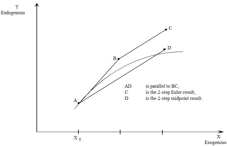
Gragg's method and the midpoint method are the same except that Gragg does one more pass. If you select N steps, midpoint does N passes while Gragg does N+1 passes. In the final (N+1)st pass, the Gragg calculation actually starts near the final point and takes the exogenous variable past its end point. This is done to obtain a correction to the result after N passes; the corrected result is usually more accurate than the one after N passes. More details about the theory behind these methods can be found in Pearson (1991) and the references therein. (Gragg's method is sometimes called the modified midpoint method7.)
Note the distinction between steps and passes for Gragg and midpoint. A Gragg 6-step calculation does 7 passes. The LOG file will refer to pass 3 of a 7-pass calculation.
Our experience is that, provided your simulation is not too nonlinear,
- Gragg or midpoint will converge significantly faster than Euler (that is, they produce more accurate results for the same number of steps), and
- the extra accuracy Gragg usually gets from the extra pass it does compared to the midpoint method is usually well worth the extra time taken.
However, we have found that in some highly nonlinear simulations, Gragg and midpoint diverge rapidly (see section 61.2.7 for an example). If this happens, the Extrapolation Accuracy Summary will tell you clearly, and you should then try Euler's method (though that may not converge either in these cases). More information about this issue is given in section 30.6.3 below.
Note that, if you are using Gragg's method or the midpoint method and are extrapolating from two or three separate calculations, all step numbers must be even or all must be odd.
(Thus extrapolating from 2,3,4-step Gragg is not allowed.) We recommend 2,4,6-step as the simplest Gragg or midpoint. (A 1-step Gragg or midpoint is really Euler, so doesn't make much sense.)
Because Gragg's method takes the exogenous variables past their simulation end-point on the final pass, it may not be suitable for some simulations of models in which it is not sensible to increase the exogenous variables in this manner. In such a case we recommend the midpoint or Euler method.
Using any of the three methods, if a percentage change variable is shocked by more than -100 per cent, this may leave its levels value dangerously close to zero after some step in the simulation. In this case GEMSIM or the TABLO-generated program will tell you that you must change the shock or the number of steps.
If you need to give a percentage change shock of exactly -100 percent (which is necessary if you want to reduce a positive value to zero in the levels), you will not be able to use Gragg's method since the levels value of this variable would be zero at the start of the final (N+1)th pass (see above). However you can use the midpoint or Euler method in this case. [This is why we have provided the midpoint method.]
30.2.0.1 Linearization method may affect results! [gpd3.12.2.2.2]
Euler's method is often described as following tangents along the function we integrate. This is true if we are dealing with a quadrature problem, i.e. the gradient is only a function of the exogenous variables (left half of 30.2).
The more general case as encountered in CGE models is, that we are dealing with ordinary differential equations(ODE). In this case the gradient is a function of both exogenous (x) and endogenous variables(y) and the gradient direction is different at every point in space (right half of 30.2).
Consider the levels equation Y = e-X. We could write the change form either as
- dY = -e-X or as
- dY = -Y
Figure 30.2 Illustration of Euler's method

It is important to notice that both sides in Figure 30.2 are showing the integration of the same levels equation written in different change forms. Comparing the two integration results shows a large difference. This illustrates the fact, that the quality of the integration result depends on the mathematical representation of the gradient.
30.3 Reusing pivots [gpd3.12.3]
For large models, the time taken for the LU decomposition (see section 30.1) of the matrix8 A(K) may be significant. (Indeed, the time taken for it may exceed the time taken for all other parts of the current step.) In this connection you should be aware that, in steps 2,3 and so on of a multi-step simulation, the Harwell sparse matrix routines can calculate the LU decomposition significantly quicker if they can make use of the position of the so-called pivots calculated when LU decomposing the corresponding matrix A(1) in step 1. This is called reusing pivots. If successful, the time taken for the LU decomposition in steps 2,3 etc is often less than half that for step 19. See Table 30.2 below for an example of the potential time saving.
Occasionally reusing pivots can reduce the numerical accuracy of solutions slightly (though this should not happen if iterative refinement is used). If you are in doubt about this, you can prohibit reuse of pivots by including the statement.
NRP = yes ; ! No Reuse of Pivots
in your Command file. The default is "NRP=no;" which means "reuse pivots".
You may also prefer to prohibit the reuse of pivots if experience shows that reuse of pivots is failing with a particular model or closure; then including "nrp = yes ;" in your Command file will save the time spent attempting unsuccessfully to reuse pivots.
Much more information about reusing pivots with Harwell routine MA48 is given in section 61.1 below.
30.4 Ignoring/keeping zero coefficients [gpd3.12.5]
Executive summary: You can include in your CMF file the line
IZ1 = no ; ! Default is YES: means ignore zero coefficients at step 1
Sometimes this can speed up multi-step calculations, since it maximizes the chances of re-using pivots. However, more (sometimes a lot more) memory may be needed. Since Release 10, GEMPACK has become much better at re-using pivots even in the default "IZ1=yes" case (see section 61.1.1). Hence, if an old CMF contains an "IZ1=no" line, it may be worth while to experiment by removing it. However, we still describe what "keeping zero coefficients" means since option IZ1 may be useful when you have a singular LHS Matrix (see section 34.1).
The following table was produced by running a 30-sector, 30-region GTAP 2-4-6 Gragg simulation with all 4 combinations of NRP and IZ1 settings. The first column (nrp=no iz1=yes) shows the default settings:
Table 30.2 Experimenting with the IZ1 and NRP options
| nrp=no iz1=yes | nrp=no iz1=no | nrp=yes iz1=yes | nrp=yes iz1=no | |
| total time (seconds) | 123 | 103 | 202 | 190 |
| Minimum MMNZ | 15,446,879 | 13,969,925 | 10,430,399 | 13,975,314 |
| MA48A time | 7 | 11 | 13*9 | 13*9 |
The conclusions are interesting (but specific to this particular simulation):
- re-using pivots (the first two columns) can halve the total time — because the costly MA48A phase (taking around 10 seconds) is done once rather than 13 times.
- the "iz1=no" option (column 2) is quicker. That is because exactly the same pivots can be reused at each step.
- The "Minimum MMNZ" row is an approximate indication of memory needed for the Harwell routines. Contrary to expectation, it seems that column 2 actually requires less memory than the default option (column 1). On closer examination it turns out that, in this case, specifying "iz1=no" makes little difference to the memory needed. It seems that the default strategy, of re-using and modifying pivots even while the sparsity pattern changes (see section 61.1), in this (JOB=1) case uses some extra memory which is about the same as that needed to store zero coefficients in the "iz1=no" case where the sparsity pattern is fixed (so that the pivots can be re-used without any modification).
You could experiment with the "iz1=no" option with your own model and simulations. However, if potential savings are only marginal, stick with the default settings.
30.4.1 More details about the "iz1=no" option [gpd3.12.5a]
GEMPACK is able to solve large systems of linear equations efficiently by exploiting the sparsity of the LHS matrices of coefficients. The Harwell sparse matrix routines (see section 30.1.2) used by GEMPACK usually only need to be told about the nonzero entries in these matrices.
Consider, for example, the "Com_clear" equations for Stylized Johansen as shown in section 4.3.3. The linearized version of these are
(all,i,SECT) XCOM(i)/100.0*p_XCOM(i) - {XH(i)/100.0*p_XH(i)
+ SUM(j,SECT, XC(i,j)/100.0*p_XC(i,j) ) } = 0
In the tableau for the Equations Matrix C (as set out in Table 3.4), notice that these two equations occupy rows 11 and 12 (see the SUMEQ map in section 79.0.1). Since only variables p_XCOM, p_XH and p_XC occur in these equations, all entries in the other columns of these rows in the tableau are necessarily zero (irrespective of the data base values). The first of these two equations (the one referring to sector "s1") can only have nonzero entries in the columns corresponding to variable components
| p_XCOM("s1") | p_XH("s1") | p_XC("s1","s1") | p_XC("s1","s2") |
(These are columns 6, 10, 12 and 14 respectively, as shown in the SUMEQ map in section 79.0.1.) The entry in the column corresponding to p_XH("s1") is -XH("s1")/100.0 which is -2/100.0 for the usual data base (as shown in Table 3.1). If however households consume none of commodity 1 (so that DVHOUS("s1"), and hence XH("s1)", are zero in the data base), this entry would be zero. This is what we mean by a zero coefficient - namely one that is zero because of the data base currently being used but might possibly be nonzero given another data base. (Contrast this to the coefficient of variable 'p_Y' in these equations which will always be zero, irrespective of the data base, since variable 'p_Y' does not appear in these equations.)
If you keep zero coefficients (in the sense just defined) during step 1 of a multi-step simulation, this maximises the chance that reusing pivots (see section 30.3 above) will succeed in steps 2,3 etc. (Since the data base changes at these steps because of updating, a zero coefficient at step 1 may possibly become nonzero in later steps.) Reuse of pivots fails (or becomes more difficult and costly) if the LHS Matrix at step 2 has an entry in a position for which no entry was recorded at step 1.) However keeping zero coefficients calculated at step 1 may increase significantly the time taken for step 1.
For many models, reusing pivots will succeed at all subsequent steps even if zero coefficients are not kept during step 1, partly because of the advanced reuse of pivots strategy described in section 61.1.1.
For some models and some simulations, reusing pivots fails unless zero coefficients are kept during step 1. In such cases, in a multi-step simulation with several steps, the extra time taken during step 1 may be more than offset by the speedup in later steps achieved by reusing pivots. (Though this would not be a consideration for a 1-step simulation and may not be for simulations with a small number of steps.)
To give you control over this, we have provided the Command file statement
IZ1 = YES|no ; ! Default YES means ignore zero coefficients at step 1
which tells GEMSIM and TABLO-generated programs whether or not to ignore zero coefficients at step 1 ["yes" says to ignore them, so "no" means to keep them]. Because we have found that keeping zero coefficients in step 1 only speeds up simulations with many steps and only for some models, "IZ1 = yes ;" is the default. If you wish to keep zero coefficients at step 1, you can include statement "IZ1 = no ;" in your Command file.
At steps 2,3 etc, recording (or keeping) all zero coefficients is usually counter-productive since it may require unnecessary amounts of memory. So the default is not to record zero coefficients at steps 2,3 etc. However, in a few cases we have found that the LU decomposition proceeds faster if all zero coefficients are kept. Hence we have provided Command file statement
KZ2 = yes|NO ; ! default is NO. "yes" means keep zero coefficients at steps 2,3 etc
which tells GEMSIM and TABLO-generated programs whether or not to keep zero coefficients at steps 2,3 etc["yes" says to keep them and "no" says to ignore them]. If reuse of pivots is failing, you may like to experiment with including the statement "KZ2 = yes ;". in your Command file to see if it speeds up calculations; however it will usually slow things down, and will almost certainly not be an improvement if reusing pivots is succeeding.
These options about IZ1 and KZ2 may be useful if you have a singular LHS Matrix — see section 34.1 for details.
30.5 LU decomposition [gpd5.5]
The CPU time taken for the LU decomposition often dominates the CPU time taken for the rest of the simulation, especially for large models10.
There are various ways in which you can experiment and possibly reduce considerably the CPU time taken for your model. Options you can try if your model is slow to LU decompose are:
- setting the starting values of MMNZ, MMNZ1 and MMNZ2 — see section 30.5.1.
- whether the memory is reallocated inside the MA48 routines or not — see section 61.2.3.
- whether to use compressions in MA48 — see section 61.2.3.1.
- whether to LU decompose the original matrix or its transpose in MA48 — see section 61.2.4.
- whether to use Markowitz pivot strategy in MA48 — see section 61.2.5.
Some other choices are mentioned at the start of this chapter. Condensation can often reduce the time to solve a model. You should check whether MA28 is faster than MA48 (and now MA48 transpose). You can adjust the level of accuracy for the your simulation. For example, it is much slower to use 10 subintervals if you find you get quite acceptable accuracy using 2 subintervals. However you would need to look at the accuracy summaries in the log file and the extrapolation accuracy file to check that the accuracy is still sufficiently good.
30.5.1 Memory for LU decomposition in simulations [gpd5.5.1]
This relates to the memory required by GEMSIM, TABLO-generated programs and SAGEM for the LU decomposition. The amount of memory allocated is controlled by the "MMNZ" number. You can specify this, or GEMPACK will guess. However, it is difficult or impossible to guess just how much memory will be needed. If (after some time) GEMPACK discovers that MMNZ is too small, MMNZ will be increased and several steps repeated — wasting some time. In practice, you need to run a simulation with the relevant model, data and closure once. The minimum suitable value for MMNZ is shown in near the end of the LOG file. Then you can insert appropriate "start with MMNZ" statements in this and other Command files with the same model, data and closure.
For example, add to CMF a line like:
start with MMNZ = 50000 ;
We suggest that you set MMNZ 10 or 20 percent higher than the minimum value otherwise the solution may take longer than necessary.
There are 3 arrays in these programs which hold entries in the LU decomposition with sizes determined by numbers MMNZ, MMNZ1 and MMNZ2.
If you use the MA48 routines (see section 30.1.2), MMNZ and MMNZ1 will be the same but MMNZ2 may be smaller.
If you use the MA28 routines (see section 30.1.2), MMNZ1 and MMNZ2 will be the same but MMNZ may be smaller.
For Release 9.0 and later, there is the Command file statement
start with MMNZ2 = <integer value> ;
This statement is available in Command files for GEMSIM, TABLO-generated programs and SAGEM.
This complements the Release 8.0 statements
start with MMNZ|MMNZ1 = <integer value> ;
(see section 32.3). You can set separate starting values for MMNZ, MMNZ1 and MMNZ2 using these three statements. In particular, it now makes sense to set separate starting values for MMNZ and MMNZ2 in some models when you use MA48.
Example: The GC10E1.CMF simulation with GTAP61 (see section 25.4.3) requires MMNZ and MMNZ1 to be at least about 202,000 and MMNZ2 to be at least about 126,000. For this simulation it would be appropriate to include the statements
start with MMNZ = 210000 ; start with MMNZ2 = 130000 ;
[Provided you have sufficient memory, it is usually a good idea to set these values slightly more than the minimum.]
In general, a statement of the form
start with MMNZ = <integer value> ;
sets all three values MMNZ,MMNZ1 and MMNZ2 to the specified value. You can set different values for MMNZ1 and MMNZ2 (if you wish) using the other two statements. [In the example above, we want MMNZ1 to have the same value as MMNZ so do not need a "start with MMNZ1" statement. But we include a "start with MMNZ2" statement since we want MMNZ2 to have a different value from MMNZ.]
30.5.1.1 Alerting about MMNZ, MMNZ1, MMNZ2 re-allocations [gpd5.5.1.1]
If MMNZ, MMNZ1, MMNZ2 need to be increased in order to finish the LU decomposition (see section 61.2.3),
- the simulation may take considerably longer than if suitable initial values for MMNZ, MMNZ1, MMNZ2 had been set via "start with MMNZ|MMNZ1|MMNZ2 = <value> ;" statements in the Command file.
- GEMSIM and TABLO-generated programs put a strong ADVICE message near the end of the run about this. [This message appears just after the minimum values for MMNZ, MMNZ1 and MMNZ2 are displayed.] Also, each time the program is doing the LU decomposition (when the message "(Calculating the LU decomposition.)" stays on the screen for a long time with a large model), the same advice is shown on the screen.
Whenever one or more of MMNZ, MMNZ1 and MMNZ2 need to be increased, you will see a report in your LOG file. [If you are using memory sharing — see section 61.3 - you will also see reports when the values of MMNZ etc are reduced.]11.
30.6 Equation solving problems [gpd3.12.6]
30.6.1 Warnings about equations not being satisfied very accurately [gpd3.12.6.1]
After solving a system of equations
A y = b
(as in equation (3) of section 3.12.2), GEMSIM or the TABLO-generated program (or SAGEM) usually calculates the product Ay (using the solution values for y) and compares it entry by entry with the RHS vector b. If these two appear to differ significantly, the program reports the equation numbers where these differences occur. The report will look something like the following12.
%%WARNING. Equation MarketClear("food","USA") is not satisfied very accurately.
(Sum of its terms is 0.2340 while sum of their absolute values is 2.230000.)
This may be because the LHS matrix is not really invertible.
If GEMSIM or your TABLO-generated program (or SAGEM) gives one or more of these warnings about equations not being satisfied very accurately, you should check the equation or equations indicated in the messages13.
You should also be suspicious of your simulation results since these messages often indicate some serious problem with the equations of your model or the closure you are using. Accordingly you should check the alleged solution carefully since it may be unreliable (or even meaningless).
Indeed, as the message says, such warnings often mean that the LHS matrix is not really invertible14. You should be aware that, in general, it is impossible to accurately distinguish numerically between a singular LHS Matrix (that is, one that is not invertible) and one that is nearly singular. (This is because of the limited precision of computers and the rounding errors that necessarily occur when doing large numerical computations.) In modelling, singular matrices are usually an indication that an invalid closure is being used, though occasionally they can be a consequence of zeros in the data base.
See section 34.1 for details about singular matrices.
Experienced GEMPACK users tend to ignore warnings since a large number are produced in many cases. However, we urge all users to take very seriously these warnings about equations not being satisfied very accurately. Indeed, if you receive more than 100 of these messages, the program runs to completion, saves all files, but then ends with a fatal error to alert you to the seriousness of the warnings
If any of these warnings is given during a simulation, a message such as the following will be given near the end of your LOG file.
%%Warning. There have been 175 warnings about equations not being satisfied very accurately. The more of these there have been, the more likely it is that the solution is not valid, indeed that one or more of the matrices is not really invertible.
The other way of checking if you have received any of these warnings is to search for
not satisfied very accurately
in your LOG file.
If, despite the above, you wish to suppress these warnings, you can do so by adding the statement.
NWE = yes ; ! No Warnings about Equations not being satisfied
in your Command file. [The default is "NWE = no ;" which means "give warnings".]
30.6.2 Warnings about variation between passes in endogenous results [gpd3.12.6.2]
If your simulation is a highly nonlinear one, you may see warnings of the following kind:
%%WARNING. Variation in endogenous values between this and the previous pass may indicate nonconvergence of the solutions. Sum of absolute values of the endogenous variables on pass 2 is 23456.0, while this sum was 78432.1 on the previous pass.
This message indicates a significant difference in the size of the endogenous results from one pass to the next one. However, by itself, this does not mean that your simulation is not converging satisfactorily.
Convergence
- is indicated best by the Extrapolation Accuracy Summaries (see section 26.2) or,
- if in doubt, by the results on the Extrapolation Accuracy file (section 26.2.3).
When you receive messages about variation between passes, you should check this Extrapolation Accuracy information carefully. If in doubt, perhaps increase the number of steps and/or subintervals used in solving the model (or use automatic accuracy). See sections 26.1 and 26.1.1 for advice about increasing accuracy.
30.6.3 Gragg and midpoint are not suitable in some cases [gpd3.12.6.3]
Gragg's method or the midpoint method converge much more quickly than Euler's method for many simulations. (That is, they produce much more accurate results for the same number of steps.)
However these methods are known to be unsuitable for some simulations because the different multi-step simulations (for example, 6-step, 8-step and 10-step) may oscillate rather than converging monotonically as we would like. In such cases, it is known that these oscillations may become worse when the number of steps in increased. You can obtain information about oscillations from the Extrapolation Accuracy file and Summary (see section 26.2).
It is virtually impossible to tell in advance which simulations will not converge with Gragg or the midpoint methods. Changing closure and especially shocks can and will change the behaviour. The practical moral seems to be the following.
If you see increasingly large oscillations in your results when using Gragg or the midpoint method, switch to Euler's method.
Euler's method does not suffer from the problem of increasingly large oscillations15.
A specific example in which there are increasingly large oscillations is given in section 61.2.7 below.
30.7 Work files [gpd3.12.7]
GEMSIM and TABLO-generated programs often produce large, temporary work files when they are carrying out a simulation. These files are usually deleted when the run is finished. However, if the program crashes, sometimes these work files are left on your hard disk.
Several of these work files have suffixes ending in WK, including .CWK, .DWK, .PWK and .SWK. Other work file suffixes are .E2K, .EXS and .EL2. It is always safe to delete such work files if you see them lying around.
Sometimes a simulation will crash with an error message suggesting that your disk is full. Usually the program cleans up the work files after such a message. This explains why you may be puzzled to find 100Mb or more free after such a message. Even if you find such a large amount of free disk space, you should try to free up more after such an error message.
The work files produced by GEMSIM or a TABLO-generated program may take up several hundred megabytes of disk space. In general, the larger your model, the larger these work files will be.
31 Solving a model in parallel on a machine with two or more processors [gpd9.2]
Click here for detailed chapter contents
Most modern PCs have dual-core or quad-core processors which incorporate several processing units in a single package. One reason for this trend is that traditional single-core CPUs have reached a performance plateau (or at least improve more slowly than before). Multi-processing offers the prospect of continued performance increases - if software can take advantage of it.
GEMPACK allows you to divide a single simulation between processors1. If you wish to solve a model by extrapolating from 2 or 3 multi-step calculations, you can ask the software to carry out one or two of these multi-step calculations in parallel with the main program. In this way you may be able to solve the model significantly more quickly than normal, as the example below shows.
The separate multi-step calculations are independent of each other. For example, if you are doing Gragg 2,4,6-step calculations, the 6-step calculation can be done independently of the 4-step calculation.
Example 1 : Gragg 2,4,6-step. Reducing time by 40-50%
Suppose you are solving using Gragg 2,4,6-step calculations. If you have two processors, you can ask the main program to carry out the 2-step and 4-step calculations. And you can ask the main program to run (on the other processor) a separate job which carries out the 6-step calculation. When that is finished, the main program will read the results from the 6-step calculation and then combine these results with the results of the 2-step and 4-step calculations to do the extrapolation and produce the usual results.
Since the 6-step calculation probably only takes as long as the 2-step followed by the 4-step, this will approximately halve the total elapsed time required to solve the model.
When you do this, we call the program you start running the master and we call the jobs it starts (the 6-step calculation in the example above) the servants.
Example 2 : Replacing Euler 4-step by more accurate Euler 2,3,4-step in same time
Suppose that you normally solve your large model using only a single Euler 4-step calculation. [This is often done with larger recursive-dynamic models.]
If you have two processors, you may now be able to carry out the more accurate Euler 2,3,4-step calculation (more accurate because of extrapolation) in about the same elapsed time as it takes to do the single Euler 4-step calculation. The master program carries out the 2-step and 3-step calculations while the servant program carries out the 4-step calculation2.
31.1 You need plenty of memory [gpd9.2.1]
When you run two or three programs in parallel (one master and one or two servants), each program requires about the same amount of memory. If your model takes about 500MB of memory to solve normally, you will need about 1000MB to run one servant or about 1500MB to run two servants. If you don't have this much memory, the servants and/or the master will be running in virtual memory (when the hard disk emulates RAM), which will make them run very slowly. Good performance requires that each running task has ample access to RAM.
However, 32-bit CPUs and 32-bit Windows can only manage 4GB of RAM.
This limits the possibility of running several memory-intensive tasks simultaneously. 64-bit CPUs and Windows versions are now available which can manage much more memory. Indeed, nearly all the dual-core or quad-core CPUs purchased now are 64-bit capable - if used in conjunction with 64-bit Windows. Hence, there is a connection between the transition to multicore PCs and the transition to 64-bit computing. That connection is explored in section 49.3.1.
31.2 Telling the program to run in parallel [gpd9.2.2]
You can do this by including the following statement in your Command file.
servants = NO|1|2 ; ! NO is the default
- "servants = 1 ;" tells the program to use one servant. The servant will do the longest multi-step calculation.
- "servants = 2 ;" tells the program to use two servants to do the longer two multi-step calculations. This only makes sense if (a) you are extrapolating from three (not two) multi-step calculations, and (b) you have three or more processors on your machine (the main program will use one processor and each of the servants ideally has its own processor).
- "servants = no ;" tells the program not to use servants. That may be appropriate even if you have two processors because you want to do serious word-processing while the simulation is running and you want the second processor to concentrate on the word processing.
31.2.1 Problems with the program deciding how many servants [gpd9.2.2.1]
It is not easy for the program to reliably discover how many processors are available on your PC. On most PCs using an Intel CPU, "hyperthreading" is enabled, which causes Windows to think that the number of processors is twice the actual value.
Although the program could find out how much memory is available on your PC, it is hard to know early on how much memory will be required to solve your model. Accordingly, the program cannot sensibly decide whether you have sufficient memory for one or more servants.
That is why, at least for the present, we require you to tell the program whether or not to use servants and, if so, how many servants to use.
31.3 Restrictions [gpd9.2.3]
-
You can only run in parallel if you are carrying out a simulation in which you are extrapolating
from two or three separate multi-step calculations. You cannot run in parallel if you are carrying
out a simulation using a single multi-step calculation or if you are running a data-manipulation
TAB file.
If you put "servants = 1 ;" or "servants = 2 ;" in a Command file which does not carry out a simulation or which carries out a single multi-step calculation, that statement will be ignored (as a note in the LOG file will indicate). [That means it is safe to put "servants = xx ;" in CMFSTART files under RunDynam and RunGTAP (see section 31.10). Such a statement will not cause an error when the software runs the model program in order to set up closures etc.] - You cannot run in parallel if you are using the memory sharing features described in section 61.3. Running in parallel is only sensible if you have plenty of memory — see section 31.1.
- You cannot run in parallel if you are starting from old Equations and SLC files — see section 59.2.
- If there are complementarity statements in your model, parallelization can only help you on the accurate run, and then only if the accurate run does not include subtotals. You should include subtotal commands on the approximate run (see section 31.6.2 for more about this).
31.4 Servants work in their own directories [gpd9.2.4]
Servant programs always work in a subdirectory of the directory in which the master program is running.
That is, servant programs produce most of their output files (and their temporary files) in a subdirectory3.
The name of the subdirectory depends on the name of the Solution file being produced by the master program and the number of the multi-step calculation the servant is doing.
Example: Suppose that the master program is running in directory c:\mymodel\32sector and that it is producing Solution file thissol.sl4 in that directory. Then, if a servant is doing multi-step calculation number 3 (the last one), it will work in the subdirectory thissol-ms3 of c:\mymodel\32sector.
The main two outputs from the servant are
- the results file which is called servant-output.sl4 and which is produced in the subdirectory in which the servant is working. [Although this file has suffix .sl4, it is not a true Solution file. For example, you cannot open it with ViewSOL. It only contains the numerical results (cumulative solution and any subtotals solutions) for one multi-step calculation. It does not contain the other information (for example, details of closure and shocks) usually contained in a Solution file.]
- the relevant updated data files, which are produced where the master would produce them if it was running normally, not as a master. These have suffixes .ud6 (for the second multi-step calculation) or .ud7 (for the third multi-step calculation). These do not go in the subdirectory in which the servant is working but in the same directory as where the master will produce the final updated file.
When the servant program finishes its run, the master program reads the results and then (normally) deletes the subdirectory in which the servant was working.
31.5 Master log file is complete [gpd9.2.5]
If you ask for a LOG file, the log file produced by the master normally includes a complete log file for each of the servants. These begin with a heading of the form
&&& SERVANT LOG &&
However:
- If there is a fatal error (see section 31.7), the master log file may not contain the log from each of the servants.
- If you are doing automatic accuracy, the master log file for each subinterval normally contains the log file from one of the servants. But if the master finds a Coefficient out of range, the master may not wait until the servants have finished before redoing the subinterval, so the log file for that subinterval may not include details from the servants.
31.6 When the servants start and finish [gpd9.2.6]
The master program carries out all of the first pass up to the point where it has solved the equations for all multi-step calculations. [The LHS is the same for each different multi-step calculation. The master calculates the two or three different right-hand sides and solves them all.]
Then it starts the servants running (and it keeps going on the first multi-step calculation).
Each servant stops when it has solved all steps relevant to its own multi-step calculation.
When the master has completed the separate multi-step calculations it is responsible for (that may be one or two multi-step calculations), it waits until the servants have all finished. Then it reads the results from the servants and continues to do the extrapolation and any post-simulation processing required.
31.6.1 If there are several subintervals [gpd9.2.6.1]
The procedure in section 31.6 above is repeated for each subinterval. The servants carry out the different steps of one multi-step calculation for a single subinterval and then stop. Then they are called into action again to do the same multi-step calculation in the next subinterval, and so on.
31.6.2 If there are complementarity statements [gpd9.2.6.2]
The approximate calculation (in each subinterval) is a single multi-step Euler calculation. The master must do this (since there is nothing for the servants to do). Only the accurate calculation can use servants to do two or three multi-step calculations.
This means that the time saving is not as great when there are Complementarity statements in the model, since there is only a time saving on the accurate run, not on the approximate run.
31.6.3 If using automatic accuracy [gpd9.2.6.3]
This is much the same as several subintervals (see section 31.6.1). The servants are called on each subinterval.
The complication (it is a considerable one) is that, if the value of a Coefficient goes out of range (see sections 6.4 and 26.4) in one of the multi-step calculations, all the others must stop and the subinterval must be done again (with a shorter length). This requires good communication between the master and the servant.
For example, if a servant detects a Coefficient out of range, it must tell the master to stop and redo the subinterval. And the master must tell the other servant (if there is one) to stop.
The other criterion used in automatic accuracy simulations is the accuracy — see section 26.4. The master is the one which does the extrapolation so it does not need to communicate with the servants when deciding whether or not to redo a subinterval because of insufficient accuracy. [This can only be decided after the extrapolation, when no servants are running.]
31.7 If a fatal error occurs [gpd9.2.7]
If one of the servants encounters a fatal error, it must stop and tell the master which must also stop. The master may not be able to immediately stop any other servants which are running. The master will give the servant instructions to stop. However the servant only checks this one or two times during each step of its multi-step calculation.
If the master encounters a fatal error, it must tell the servants to stop and then stop itself. Again the master will instruct each servant to stop - but again the instructions may not be obeyed immediately.
31.8 Fine print [gpd9.2.8]
31.8.1 Displays and writes to terminal at all steps [gpd9.2.8.1]
This relates to option DWS or Command file statement "dws = yes ;" — see section 25.1.10.
A master program will do as requested. But any servant programs it runs will not do any Displays. However servant programs will do writes to the terminal for all steps that they carry out (as will the master program).
31.8.2 Multi-step calculations may not be independent of each other [gpd9.2.8.2]
With the new (Release 10) re-use of pivots strategy (see chapter 61.1), the separate multi-step calculations are not completely independent of each other — see the first footnote to point number 2 in section 61.1.1.
31.9 Some elapsed times [gpd9.2.9]
In this section we report some elapsed times with and without servants for various models with different compilers.
All times reported here were obtained on a Windows XP PC with two dual-core AMD64 Opteron 270 2.01GHz chips (that is, 4 processors) with 8GB of physical memory.
The times for the LF90, LF95 and Intel-32 compilers were obtained running under the Windows XP Professional (32-bit) operating system. The times for the Intel-64 compiler were obtained running under the Windows XP Professional x64 Edition (64-bit) operating system.
In each case, the default compiler options as supplied with Release 9.0 of GEMPACK were used. For LF90 and LF95 this is basically O1 optimisation options (the same as for Release 9.0 of GEMPACK with these compilers). For the Intel compilers, this was /O2 optimisation option (which is also the default recommended by Intel)4.
The times reported are elapsed times. Even for the same compiler and Command file, the elapsed time varies from run to run5. The times reported are the average of 3 runs in each case.
The version of GTAP is one with 38 regions and 39 tradeable commodities. The simulation in SIM1.CMF is a Gragg 2,4,6-step simulation.
The version of GTEM used for the report below has 23 regions and 29 tradeable commodities. [This is the same version of GTEM we reported about in chapter 30.5.] GTEMSIM3.CMF is an Euler 3,5,7-step simulation.
The TERM-WATER version is a version of TERM with 48 commodities and 20 regions aimed at water-related applications. This is the TERM model reported in the tables in section 61.2.4. This model contains Complementarity statements. TERMSIM1.CMF does 3-step Euler approximate run followed by Euler 2,3,4-step accurate run. There are no Complementarity state changes in this simulation.
31.9.1 Comments on the elapsed times reported [gpd9.2.9.1]
The best you can hope for is that, by using 2 servants, the elapsed time will be the same as the elapsed time for the longest of the 3 separate calculations. As you can see from the last two columns in Table 31.9, that pretty much happens (except for the LF90 GTAP simulation).
With one servant, the master does the shorter two multi-step calculations while the servant does the longest multi-step calculation.
Gragg 2,4,6 Example
In the case of the Gragg 2,4,6 GTAP simulation, this means that the master does something like 2+4=6 passes while the servant does 6 passes. [A Gragg 4-step has 5 passes. The first pass of all multi-step calculations is done by the master before the servant starts. So the servant does the last 6 passes of the 7-pass Gragg 6-step while, starting at the same time, the master does the last 2 passes of the Gragg 2-step and then the last 4 passes of the Gragg 4-step.] On the basis of this (crude) analysis, you might expect that the master would finish its two tasks (Gragg 2 and 4) at about the same time as the servant finished its one task (Gragg 6). In fact, in this simulation, the master takes longer than the servant because of variations between the times taken for the different steps6.
The TERM-WATER simulation has a 3-step Euler approximate run followed by an Euler 2,3,4-step accurate run. The master does all of the approximate run (the servants are not able to help with that). Hence the overall time saving is not as great as for the other simulations reported.
Table 31.1 Elapsed times for typical simulations with and without servants
| Simulation and Compiler | Simulation(no servants) | 1 Servant | 2 Servants | Longest multi-step calculation |
| GTAP38X39 SIM1.CMF | Gragg 2,4,6 | Gragg 6 | ||
| LF90 | 48m 35s | 32m 18s | 26m 39s | 20m 57s |
| LF95 | 66m 24s | 35m 19s | 34m 58s | 33m 58s |
| Intel 32 | 48m 10s | 26m 28s | 23m 49s | 23m 40s |
| Intel 64 | 41m 23s | 24m 55s | 21m 32s | 20m 48s |
| GTEM GTEMSIM3.CMF | Euler 3,5,7 | Euler 7 | ||
| LF90 | 17m 31s | 10m 51s | 10m 21s | 10m 14s |
| LF95 | 46m 8s | 25m 32s | 24m 57s | 24m 19s |
| Intel 32 | 19m 43s | 11m 3s | 10m 57s | 10m 45s |
| Intel 64 | 18m 20s | 10m 39s | 10m 38s | 9m 54s |
| TERM-WATER TERMSIM1.CMF | Euler 2,3,4 (+3-step approx run) | Euler 4 (+ 3-step approx run) | ||
| LF90 | 6m 33s | 4m 38s | 4 m 32s | 4 m 33s |
| LF95 | 7m 34s | 5m 28s | 5m 32s | 5m 15s |
| Intel 32 | 5m 23s | 3m 38s | 3m 27s | 3m 37s |
| Intel 64 | 3m 58s | 2m 50s | 2m 50s | 2m 45s |
Summary
- If you have 3 or more processors and run with 2 servants, you can expect that the elapsed time will be roughly that for the longest multi-step calculation.
- If you have only 2 processors (or run with only one servant), you still can expect to make considerable time savings. And you can estimate how much by considering how many total passes the master and servant must each make (once the servant is started).
Fine Print
The times reported in Table 31.9 were obtained before the new re-use of pivots strategy (see chapter 61.1) was introduced.
31.10 Using master/servant under RunDynam [gpd9.2.10]
You can instruct RunDynam etc to use a master and one or two servants for each solve. To do so, include the relevant statement
servants = x ; ! x is 1 or 2
in your CMFSTART file(s).
Your PC will need more memory to use servants, since the master and each servant need the same memory as a single run of the model (see section 31.1). So if you want to run efficiently with one servant, you need to have available on your computer at least twice the memory necessary for one solve of the model. [Otherwise the 2 programs will be fighting each other for memory and the master plus servant may end up taking longer than if you ran without a servant.]
RunDynam etc can now run up to 3 jobs concurrently. Each job requires its own memory. So if you wish to run 3 concurrent jobs efficiently, you need to have available on your computer at least 3 times memory necessary for one solve of the model. [Otherwise the 3 programs will be fighting each other for memory and the 3 jobs concurrently may end up taking longer than if you ran them one after the other.]
If you want to combine concurrent solves and master/servant under RunDynam, you have to be even more aware of the memory requirements.
Example
Suppose, for example, you click on the Run All button of RunDynam and that you are allowing 3 concurrent solves (under the RunDynam Options menu) and have specified each simulation to use a master and one servant. Then for efficient running you need to have available on your computer at least 6 times the memory necessary for one solve of the model.
32 Memory management [gpd3.13]
Click here for detailed chapter contents
In this chapter we describe aspects of memory allocation and management for GEMSIM, TABLO-generated programs and SAGEM which you may need to understand in order to ensure that these programs carry out simulations as quickly as possible.
32.1 Automatic memory allocation [gpd3.13.1]
GEMPACK programs allocate just enough memory to complete each task. If there is not sufficient memory available on your computer, the programs will stop with a message that it is unable to allocate sufficient memory.
This memory allocation is done when the sizes of the relevant arrays are known.
32.2 Preliminary pass [gpd3.13.2]
When GEMSIM or a TABLO-generated program run, they perform what they refer to as a "preliminary pass" in which they calculate the sizes of all sets and compute all subset mappings. On this pass they only do whatever is required to get this information. For example, they only do FORMULAs if some set is dependent on the values of a particular COEFFICIENT (see section 11.7.6).
32.3 MMNZ: Allocating memory for the LU decomposition [gpd3.13.3]
Memory is allocated for the LU decomposition. The amount of memory allocated is controlled by the MMNZ number. You can specify a starting value for MMNZ in a command file, or GEMPACK will guess. However, it is difficult or impossible to guess just how much memory will be needed. If (after some time) GEMPACK discovers that MMNZ is too small, MMNZ will be increased and several steps repeated -- wasting some time. To determine a useful value for MMNZ, you should run a simulation with the relevant model, data and closure, then look for the minimum suitable value for MMNZ shown near the end of the LOG file. Then you can insert appropriate "start with MMNZ" statements in this and other Command files with the same model, data and closure. See section 30.5.1 for more details.
32.4 Reporting memory used by TABLO-generated programs and GEMSIM [gpd3.13.4]
GEMSIM and TABLO-generated programs produce a fairly accurate estimate of the total memory needed. If this amount is more than (or, even close to) the total amount of physical memory on your computer, you should consider using the memory sharing option described in section 61.3 below.
These programs allocate all the memory they think they will need early in the run (after the preliminary pass). As the number of nonzeros in the system becomes known, more memory may be allocated by increasing values of MMNZ, MMNZ1 and MMNZ2 — see sections 32.3 and 30.5.
Each time MMNZ, MMNZ1 or MMNZ2 is increased, a report is given showing the total memory required so far. A final report showing the total memory required is given near the end of the run1.
These reports are as follows:
Total memory currently used for all arrays is approximately 316.13 megabytes.
[This includes memory relating to current values:
MMNZ=11929376, MMNZ1=11929376 and MMNZ2=11929376.]
[Add about 5-10 megabytes for the memory used by the code.]
[This is probably the most memory that will be used in this run.]
32.4.1 RunDynam manages MMNZ start values [rundynam.mmnz]
From RunDynam version 3.57 (December 2010), by default RunDynam attempts to manage the "start with MMNZ" values. [This can be switched off with the "Manage MMNZ" item in the RunDynam "Run Preferences" menu.] RunDynam gets information about the values needed in each simulation period and uses that information for subsequent simulation periods. RunDynam does this by adding its own "start with MMNZ" statements to the Command file it creates and comments out any "start with MMNZ" statements in the files you supply.
32.4.2 TGMEM1 and TGMEM2 parts of memory [gpd3.13.4.1]
GEMSIM and TABLO-generated programs also report the size of so-called TGMEM1 and TGMEM2 parts of memory used. These reports indicate what is included in these parts of total memory. For large models, the TGMEM1 part is usually the larger of these.
Note that these reports do not include memory required for the nonzeros generated doing the LU decomposition (where memory is allocated according to the size of the parameters MMNZ and MMNZ1).
33 Options for GEMSIM and TABLO-generated programs [gpd3.14]
Click here for detailed chapter contents
GEMSIM and TABLO-generated programs offer several different options, which can affect the way they run (for example, how they carry out a simulation).
The options screen for TABLO-generated programs is shown below1.
TABLO-GENERATED PROGRAM OPTIONS
( --> indicates those in effect )
BAT Run in batch STI Take inputs from a Stored-input file
BPR Brief prompts SIF Store inputs on a file
LOG Output to log file ASI Add to incomplete Stored-input file
CMF Take inputs from a Command file
EAA Echo all activity SVX Select variables on XAC file (later)
CPU Report CPU times RQF Required figures agreement (extrap)
NRP Don't reuse pivots NIR Don't do solution iterative refinement
-->IZ1 Ignore zero coefficients in step 1
KZ2 Keep zero coefficients in steps 2,3 etc
NEQ Do no equations NWE Don't warn how well equations solved
NDS Do no displays SSI Several subintervals; extrap after each
NWR Do no writes M28 Use MA28 routines (rather than MA48)
NAS Do no assertions SUI Save updated formula(initial) data
NUD Do no final updates Extra Options Screen
NSM Don't do simulation --------------------
NWT Use Newton's method DTO Display, Terminal/Text write Options
CR Check-on-read options
Select an option : <opt> Deselect an option : -<opt>
Help for an option : ?<opt> Help on all options : ??
Redisplay options : / Finish option selection : Carriage return
Your selection >
The options screen for GEMSIM is the same.
Note that, in both cases, option IZ1 is selected by default2 (though you can, of course, turn it off).
As indicated in section 48.4.2, Help screens can be displayed while running these programs by typing '?' followed by the abbreviation to the option on which help is needed. For example, to obtain help on Log files, type ?LOG. To obtain help on all options, type ?? and scroll through the screens using a carriage-return. However, unless you are doing something special, you should probably use the default options plus the option CMF.
For this reason, you may prefer to skip chapter 33 initially and only return to it later if and when you feel you need the more specialised information and advice given below.
Most of the options described below can be activated by appropriate statements in GEMPACK Command files; we mention the related Command file statements when discussing the options below.
33.1 Options affecting simulations [gpd3.14.1]
Several of the options available with GEMSIM and TABLO-generated programs affect the way simulation results are calculated. Some of these are aimed at possibly speeding up the calculations.
The relevant options (with their Command file equivalents also shown) are:
| IZ1 | Ignore zero coefficients in step 1 | ("IZ1 = yes ;" in Command files) |
| KZ2 | Keep zero coefficients in steps 2,3 etc | ("KZ2 = yes ;" in Command files) |
| NRP | Don't reuse pivots | ("NRP = yes ;" in Command files) |
| NIR | Don't do solution iterative refinement | ("NIR = yes ;" in Command files) |
| NWE | Don't warn how well equations solved | ("NWE = yes ;" in Command files) |
| NWT | Use Newton's method | ("NWT = yes ;" in Command files) |
| SSI | Several subintervals: extrap after each | ("subintervals = <number> ;" in Command files) |
The effects of IZ1 and KZ2 are described in section 30.4. The effects of NRP, NIR and NWE are described in sections 30.3, 30.1 and 30.6.1 respectively. The effect of NWT is described in section 26.6. The effect of SSI (several subintervals) is described in section 26.3.
33.2 Options affecting extrapolation accuracy summaries and files [gpd3.14.2]
The relevant options (with their Command file equivalents also shown) are:
| RQF | Required figures agreement (extrap) | ("RQF = <integer> ;" in Command files) |
| SVX | Select variables on XAC file (later) | ("xac-retained endogenous = <list> ;" in Command files) |
These are described in section 26.2.6.
33.3 Saving updated values from all FORMULA(INITIAL)s [gpd3.14.3]
The option
| SUI | Save Updated values from formula Initials | ("sui = yes ;" in Command files) |
in GEMSIM and TABLO-generated programs allows you to save updated values of all coefficients whose initial values are set via FORMULA(INITIAL)s. See section 26.8.2 for details.
33.4 Options affecting the actions carried out [gpd3.14.4]
These can be used to suppress actions that GEMSIM or the TABLO-generated program is capable of carrying out. The relevant options are shown below. Each has a Command file equivalent (which you should prefer to use as a general principle) which is also shown.
| NEQ | Do no equations | ("NEQ = yes ;" in Command files) |
| NDS | Do no displays | ("NDS = yes ;" in Command files) |
| NWR | Do no writes | ("NWR = yes ;" in Command files) |
| NUD | Do no final updates | ("NUD = yes ;" in Command files) |
| NAS | Do no assertions | ("assertions = no ;" in Command files) |
| NSM | Don't do simulation | ("simulation = no ;" in Command files) |
The effects of NDS, NWR, NAS, NUD, NEQ and NSM are described in section 25.1.8 above.
33.5 Options affecting how writes and displays are carried out [gpd3.14.5]
There are several options affecting how writes to text files and displays are carried out.
If you are running interactively or via a Stored-input file, you can see these options by first selecting option
| DTO | Display, Terminal/Text write Options |
This reveals the following menu.
DISPLAY/TERMINAL/TEXT FILE OPTIONS
( --> indicates those in effect )
DWS Displays, terminal writes at all steps of a multi-step sim
TWC Terminal writes in column order
DPW Change page width of display file
DPL Change page length of display file
DDC Change number of figures after decimal point in displays
--> DPN New page in display files only if needed
D1C In display files, show 1-dimensional array as a column
DOI In display files, omit "identical" row messages
NEL No element labels on ROW_ORDER or COL_ORDER text files
Select an option : <opt> Deselect an option : -<opt>
Help for an option : ?<opt> Help on all options : ??
Redisplay options : / Return to other Options : Carriage return
Your selection >
Once you have selected any options desired from this, you return to the main options menu by entering a carriage-return.
Alternatively, if you are using a GEMPACK Command file, you can select these options directly - option DTO is not relevant. For example, "display width = 70 ;" sets the width of pages in the display file to 70.
Options DWS and TWC are equivalent to the Command file statements "dws = yes ;" (see section 25.1.10) and "twc = yes ;" (see section 25.1.12).
Display files are introduced in section 22.3. Options DPW, DPL, DDC, DPN, D1C and DOI are the analogues of the respective Command file statements described in section 22.3.
Normally element name or number labels are shown (as comments) in row_order or col_order text data files (see section 38.2.14). If you select the option
| NEL | No element labels on ROW_ORDER or COL_ORDER text files |
or put the statement "NEL = yes ;" in your Command file, such labels will be suppressed. (See chapter 38 for more information about these GEMPACK text data files.)
33.6 Options affecting CPU and activity reporting [gpd3.14.6]
The relevant options (with their Command file equivalents also shown) are:
| CPU | Report CPU times | ("CPU = yes ;" in Command files) |
| EAA | Echo All Activity | ("EAA = yes ;" in Command files) |
These options are described in sections 20.6 and 25.1.11 respectively.
33.7 Special options for SAGEM [gpd3.14.7]
Several options are available for SAGEM apart from the basic options BAT, LOG etc (which are described in chapter 48). For SAGEM, these are CPU, CMF, NSM, NIR, NWE and KZC. These extra options are described below. However you will find that the default options (that is the program settings you get if you do not choose any options) are suitable in most standard cases.
Note that, as for any other GEMPACK program (see section 48.4.2), Help is available. For example, to find information about the SAGEM option NIR, just respond '?NIR' when prompted for your choice of options. Responding '??' will give Help for all options.
33.7.1 SAGEM options [gpd3.14.7.1]
SAGEM can be run using a Command file. To do this, select option
| CMF | Input from a GEMPACK Command file |
and give the name of the Command file. Further details are given in section 35.4 about preparing Command files for SAGEM and their syntax. We recommend that you always run SAGEM from a Command file.
Usually SAGEM carries out iterative refinement of the solutions to improve their accuracy. However you can turn iterative refinement off using option
| NIR | Don't do solution iterative refinement | ("NIR = yes ;" in Command files) |
See section 30.1 for more details.
If you only wish to set up the closure for a simulation and then save it on an Environment file (see section 23.2), select
| NSM | No simulation (closure only) | ("simulation = no ;" in Command files) |
The Environment file created can then be used in later simulations to specify the closure.
Select option
| CPU | Report CPU times | ("CPU = yes ;" in Command files) |
to obtain processing times for the five stages of a simulation:
- User specification of the simulation,
- Creation of the right-hand side matrix, that is, the matrix B in equation (3) of section 58.1,
- Creation of the Left Hand Side Matrix, that is, the matrix A in equation (3) in section 58.1,
- LU decomposition of the Left Hand Side Matrix, and
- Calculation and writing of solutions.
Alternatively, deselect the CPU option ("CPU = no ;" in Command files) to omit CPU time reporting.
Normally warnings are given to indicate how well the equations have been satisfied — see section 30.6.1 for details. Option
| NWE Don't warn how well equations solved | ("NWE = yes ;" in Command files) |
will suppress these warnings. However, you should take these warnings very seriously (see section 30.6.1) so we advise you not to suppress them.
KZC Keep zero coefficients ("KZC = yes ;" in Command files)
Zero coefficients are entries in the Equations Matrix which are calculated to be zero from the current data base but may be non-zero for some other data base. Normally zero coefficients are not saved for SAGEM simulations. However it may help the LU decomposition in some models to save them. See also section 30.4 for a further discussion of zero coefficients and similar options in GEMSIM and TABLO-generated programs.
34 Run-time errors [gpd3.15]
Click here for detailed chapter contents
Most of the error messages reported by GEMSIM or TABLO-generated programs will be self-explanatory. Below we give information about situations in which you may need more details in order to rectify the problem.
These are when the simulation fails
- because of a singular matrix,
- because of a divide-by-zero error, or
- because of invalid values in powers or in functions such as LOG, or
- because of some other arithmetic problem such as overflow.
These are discussed in sections 34.3.
There are other reasons why a simulation may not run to completion.
- See section 21.4 for checks that the Auxiliary files match the TABLO-generated program.
- See section 22.4 for checks on the set and element data when reading data.
- For details on equations-solving problems see section 30.6.
See also the Frequently Asked Questions section of the GEMPACK Web site at address:
http://www.copsmodels.com/gp-faq.htm
34.1 Simulation fails because of a singular LHS matrix [gpd3.15.1]
Your simulation may fail because the Left Hand Side Matrix (that is, the matrix A in the equation1 A y = b) is singular (that is, not invertible) at some step. A singular matrix is either an indication
- that the closure you are using is not valid (even though it has the required number of exogenous and endogenous variables — see section 23.2.7), or
- of zeros in your data base, or
- that at least one linearized equation is a linear combination of other equations present in your model.
The Harwell sparse matrix routines (see section 30.1) distinguish between structurally singular and numerically singular matrices, and an understanding of the difference may help you sort out the problem.
To see the difference between these, consider the (extremely uninteresting) model with just one linearized equation
EQUATION (all,i,COM) D(i)*s(i) = t(i) ;
where COM is the set (c1, c2) and the two values of coefficient D are read from the data base. Consider the closure in which both components of variable t are exogenous and both components of variable s are endogenous. In this case the Left Hand Side Matrix A (see section 3.12.2) will be
( D("c1") 0 )
( 0 D("c2") ).
Clearly A is invertible if and only if D("c1") and D("c2") are both nonzero.
Suppose now that D("c1") is zero and D("c2") is nonzero. Then the matrix A will be singular. Whether it is reported to be structurally or numerically singular depends on whether you are "keeping zero coefficients" in the Equations file, in the sense explained in section 30.4 above. If you are keeping zero coefficients, A will have two entries (that is, possibly nonzero entries), so that A has the shape
( * 0 ) ( 0 * )
and A will be reported as being numerically singular. This means it is singular but might be nonsingular for different values of the entries (those marked * above). If, on the other hand, you are not keeping zero coefficients so that A has the shape
( 0 0 ) ( 0 * ).
then A will be reported to be structurally singular. This means that there are no values of the entries (marked * above) which could make the matrix invertible. See also section 34.2 for another definition of structurally singular.
Thus, if you find that the LHS Matrix is structurally singular, and if you are keeping zero coefficients in the current step, this means that the matrix will never be invertible, whatever values you have on the data base, which suggests that your closure is invalid. If, on the other hand, it is numerically singular and you are keeping zero coefficients in the current step, this means that it might become invertible if you changed your data.
This is another reason for us providing options IZ1 and KZ2 (see section 30.4 above). If the LHS Matrix is reported as being structurally singular at step 1 and you are using the default option IZ1, you may want to run the program again, this time deselecting option IZ1 (that is, putting "IZ1 = no ;" in your Command file). If the matrix is then reported as being numerically singular, this indicates that the closure might be valid and may be failing because of the particular values in your data base. Similarly, it may occasionally help to select option KZ2 (that is, put "KZ2 = yes ;" in your Command file) if the singular matrix is at step 2 or more.
34.1.1 Trying to fix a singular matrix problem [gpd3.15.1.1]
The problem of a singular matrix, either structurally singular or numerically singular, can be tricky to analyse and fix. There is no fool-proof general-purpose method for tracking down and eliminating these problems.
However there are several thing you can try.
- If you are working with a model which has a standard closure or some closure that is non-singular, start from that closure and use swaps to move towards the troublesome closure. Make one swap at a time. The first time you get a singular matrix, examine carefully the last swap to try to identify the problem.
- Examine the rank of the matrix if this is printed out as part of the error message. The rank for a non-singular matrix should be equal to the number of endogenous variables you are solving for. For a singular matrix, the rank is less than the number of endogenous variables (and the difference is called the rank deficiency). This gives you some indication of the number of equations which are not independent. Suppose you are dealing with a model containing sets COM and IND of sizes 40 and 38 respectively. If the rank deficiency is 40, then you can try making swaps of vector variables defined over the set COM to try to remedy the problem. On the other hand, if the rank deficiency is 38, maybe a swap of vector variables defined over IND is required. If the rank is only one or two short, you can try swapping macro variables.
-
If the rank is just a few less than the number of endogenous variables, the problem may be caused
by just one or two zeros in your data. For example, if you are using the equation
(all,k,COM) P(k) * y(k) = Q(k)*z(k)
to solve for the variable y(k), this is only valid if the coefficient P(k) is non-zero for all values of k in the set COM. There may be just the occasional value of k where P(k) is zero and this may be causing the singularity of the matrix. You may be able to overcome the problem by changing the value of a data item P(k) from zero to a small nonzero value. - Consider switching the values of options IZ1 and KZ2, as discussed in section 34.1 above.
-
If your matrix is numerically singular, you may gain more information by switching to the
alternative sparse-solving routines.
If you are using MA48, try using MA28 by putting the statement "m28=yes ;" in your Command file.
If you are using MA28, try using MA48 by putting the statement "m28=no ;" in your Command file.
However if the model is singular with one of these but not with the other, you should be highly sceptical about the validity of the results. You may find that the results are nonsense. - If you have different data sets for the same model it may help to try the same closure with a different aggregation. If the model solves with slightly different data, zeros in the data may be the cause of your numerical singularity.
- If you are building a new model, it may be easier to build it in modules and obtain a closure step by step in the course of development.
- Equation-solving problems as described in section 30.6 may be caused by a matrix which is very nearly singular.
- Look at the following section 34.2 for more details on structural singularities.
34.2 Structurally singular matrices [gpd3.15.2]
In this section we give information which may be relevant if the LHS Matrix is structurally singular.
Recall that the determinant of an NxN matrix is the sum of N! (that is, factorial N) terms, each term being plus or minus a product of N entries from the matrix, one entry from each row and one from each column.
For example, the determinant of the 3x3 matrix A with entry aij in row i and column j is equal to the sum of the 6 terms
a11 a22 a33 - a11 a23 a32 - a12 a21 a33 + a12 a23 a31 + a13 a21 a32 - a13 a22 a31
The structural rank R is defined as the maximum number of nonzero entries aij where at most one entry is counted from each row and at most one entry is counted from each column. The structural rank of the matrix tells you how far the matrix is from being invertible. Any invertible NxN matrix has nonzero determinant and so has structural rank equal to N.
For example, the 3x3 matrix whose nonzero entries are shown by * below has structural rank 2.
| [ * | 0 | 0 ] |
| [ * | * | * ] |
| [ * | 0 | 0 ] |
There are several ways of taking 2 nonzero entries from different rows and columns from this matrix. For example, a11 a22 or a11 a23 or a31 a22 or a31 a23 but it is not possible to find 3 such nonzero entries.
When the LHS Matrix is structurally singular, it is not possible to solve the model (with the given closure and data).
The difference between N (the number of endogenous variables) and R (the structural rank) tells how far the LHS Matrix is from being invertible. This difference is sometimes called the rank deficiency.
Suppose that the LHS Matrix is structurally singular and that the rank deficiency is equal to D. Then it is possible to identify D variables and D equations with the following properties2 :
(1) If you use the N equations to solve for the remaining N-D variables, it is not possible to solve for any of the identified D variables.
(2) The D identified equations add no information to the remaining N-D equations in the sense that, if you used the remaining N-D equations to solve for the remaining N-D variables, the D equations cannot be used to solve for any of the identified D variables3.
For example, consider the structurally singular 3x3 matrix above with structural rank 2. Suppose that the equation names are eq1, eq2 and eq3 associated with the 3 rows (in order) and that the variable names are x1, x2 and x3 associated with the 3 columns (in order)4.
- If you used the first 2 equations to solve for x1 and x2, it is not possible to use the third equation eq3 to solve for the remaining variable x3. Hence variable x3 and equation eq3 are one variable/equation pair which might be identified.
- Equally well, if you used the last 2 equations to solve for x1 and x3, it is not possible to use the first equation eq1 to solve for the remaining variable x2. Hence variable x2 and equation eq1 are another variable/equation pair which might be identified.
Thus, although D variables and equations can be so identified, there is nothing unique or special about the variables and equations so identified. So, although GEMPACK identifies D such variables and equations when the LHS Matrix is structurally singular, we suggest that you do not place too much emphasis on the exact variables and equations.
34.2.1 Solving modified equations when LHS matrix is structurally singular [gpd3.15.2.1]
When GEMSIM or a TABLO-generated program finds a structurally singular LHS Matrix on the first step of a simulation, it reports the structural rank R and the rank deficiency D and identifies (one) set of D variables and equations as described above.
You can ask the software to try to solve a modified system of equations (as described below). We offer this possibility since, once you have a solution, you may be able to use the relevant tools (for example, ViewSOL and/or AnalyseGE) to assist you to find the cause of the singularity. If you request the software to solve the modified equations, you should be aware that the solution produced is NOT the solution to your original model and so should be treated with appropriate caution.
To request the software to solve a modified system, you need to add the statement
structurally singular solve modified equations = yes ;
to your Command file. The default is "no".
The modified system of equations is produced as follows. The D variables identified (see above) are given the value zero. The D equations identified (see above) are modified to ensure that the D identified variables are given the value zero. The software attempts to solve the modified system which consists of the remaining N-D equations plus the D modified equations.
For example suppose that the D variables identified are the last D variables and that the D equations identified are the last D equations. Then the original LHS Matrix will be of the form
| [ | M1 | M2 | ] |
| [ | M3 | 0 | ] |
where M1 is RxR, M2 is RxD and M3 is DxR. The 0 block is of size DxD. The entries must be all zero here or else the structural rank would be more than R.
In this case, the modified system of equations solved has LHS Matrix equal to
| [ | M1 | M2 | ] |
| [ | 0 | I | ] |
where I denotes the DxD identity matrix (all diagonal entries are 1, all off-diagonal entries are zero).
If the original RHS vector is equal to
| [ | B1 | ] |
| [ | B2 | ] |
where B1 is of size Rx1 and B2 is of size Dx1, then the modified RHS vector is set equal to
| [ | B1 | ] |
| [ | 0 | ] |
The lower 0 block of size Rx1 ensures that the identified D variables have value zero when the modified system is solved.
The resulting modified system may still be numerically singular (but should not be structurally singular).
A case where the solution to the modified equations may be helpful is where you are checking the homogeneity of a model (see section 79.1). If the rank deficiency is small (it may be just 1), the identified D variables will only occur in a small number of the equations. Hence the solutions for the other variables in the modified system may be very similar to what you would have obtained if you had been able to solve the original equations. Accordingly you may still gain useful information from the solution to the modified equations.
We have had only limited experience with solving a modified system, and welcome correspondence from users who try it. We will be interested to hear if the modified solution was helpful or a hindrance.
34.3 Reporting arithmetic errors [gpd9.7.4]
This relates to the reporting of overflow5 or other arithmetic errors which occur while doing a Formula, Submatrix, Backsolve or Update. GEMSIM and TABLO-generated programs report all instances of the following types of errors.
- division by zero when this is not allowed.
- using invalid powers (for example, a negative value raised to a non-integer power).
- evaluating functions at invalid values (for example, the LOG of a negative number).
- arithmetic overflow (either real or integer overflow).
GEMSIM and TABLO-generated programs write a detailed arithmetic error report in the Log file from the run6. The arithmetic error report contains
- the type of error.
- the type of statement (Formula, Update etc) and the line number in the TAB file on which the statement which produced the error can be found.
- the name of an automatically generated HAR file from which the values of the Coefficients and Variables in the expression containing the error may be read. The values shown in that HAR file are those for the Coefficients/Variables involved in the relevant step of the multi-step calculation.
Variables can only occur if the error occurs in a Backsolve, Update or (see chapter 12) in a postsim Formula7.
For the first 3 types of errors listed above (but not type 4- arithmetic overflow), the arithmetic error report also contains
- the values of the active indices (if any) for the first occurrence of the error.
- the full expression being evaluated when the error occurred.
- the values directly involved when the error first occurred (for example, the value of the numerator in the case of a division by zero error, or the value of the argument in the case of an invalid function argument).
- the expression(s) directly involved in the error (for example, the expressions for the numerator and the denominator in the case of a division by zero error). However, these expressions are not shown when the error occurs doing a submatrix because, at present, we are unable to accurately report these expressions in that case. See Example 3 below.
Of course it is possible for several errors of type 1-4 above to occur in a statement. If so, the report only gives details (values of indices) for the first case. For example, if a formula ranges over set COM and erorrs occur doing the 4th and 8th elements of COM, details will only be given for the 4th one since that is done first.
We give several examples below.
If the arithmetic error report indicates that the error occurred
while completing update of Coefficient "<name>"
please also see section 34.3.1 below.
Fixing an arithmetic error problem may involve changing the formula or equation in question to allow for zeros in the data, or involve adding appropriate ZERODIVIDE statements (see section 10.11) to the TABLO Input file, or it may involve changing the base data and/or closure.
Example 1 — Divison by zero in a Formula
You can engineer a simple division by zero error by modifying the Stylized Johansen model (see 4.3.3) by inserting the line "FORMULA PC("s2") = 0 ;" immediately after line 116 so that lines 116 and 117 now read
FORMULA (all,i,SECT) PC(i) = 1.0 ;
FORMULA PC("s2") = 0 ;
The FORMULA & EQUATION beginning on line 131, repeated below, contains a division by PC(i) which will be division by zero when i="s2":
FORMULA & EQUATION Comin # Intermediate input of commodity i to industry j # (all,i,SECT)(all,j,SECT) XC(i,j) = DVCOMIN(i,j) / PC(i) ;
Running the model with the command file sjlb.cmf results in an error. The Log file sjlb.log from the run contains the arithmetic error report shown overleaf.
The report tells you the relevant line number in the TAB file, the arithmetic error type (division of nonzero by zero), the value of the numerator, the values of the indices involved, the numerator and denominator expressions (since the operation is division) and the complete expression. The automatically generated HAR file sjlb-assert-arith-fail.har contains the values of the two Coefficients DVCOMIN and PC which appear in the expression that produced the error.
Arithmetic error report
-----------------------
%% Error doing formula for coefficient "XC",
at line 131 in the TAB file.
Division of a nonzero by zero when this is not allowed.
This occurred first when:
nonzero numerator=2.0000000
(There are 2 active indices)
index "i" from set "SECT", value "s2" (element 2)
index "j" from set "SECT", value "s1" (element 1)
Expression for numerator is:
DVCOMIN(i,j)
Expression for the denominator is:
PC(i)
Expression being evaluated is:
(ALL,i,SECT) (ALL,j,SECT) XC(i,j) = DVCOMIN(i,j) / PC(i)
(Written real array, size 2, header '0001'.)
(Written real array, size 2x2, header '0002'.)
[Have written Coefficient values to headers "0001" to "0002"
of file "sjlb-assert-arith-fail.har".]
This occurred doing formula for coefficient "XC",
at line 131 in the TAB file.
[See Section 34.3 of the GEMPACK Manual, "Reporting arithmetic errors".]
[TopicID:gpd9.7.4]
If you have a log file search for "Arithmetic error report" to locate the
start of the report.
End of arithmetic error report
------------------------------
Example 2 — SQRT in a Formula
Consider the Formula
Formula (all,c,COM) COEF1(c) = SUM(i, IND, C2(c,i) + SQRT[C3(c,i)+C4(c)]) ;
Suppose that, on step 3 of a multi-step calculation, the values are such that the expression inside the SQRT is negative (which is not allowed). Then the program will report an error. Amongst other things it will tell you that the expression involved as the function argument is
C3(c,i) + C4(c)
The values of the indices for which that expression is negative (and the negative value) will be indicated. The values of all RHS Coefficients C2, C3 and C4 during step 3 (all of these values, not just those for the indices for which the error occurred) will be shown in the relevant assert-arith-fail HAR file.
If you use BADSQRT.TAB and BADSQRT.CMF supplied with GEMPACK, you will be able to see the arithmetic error report.
Example 3 — Division by zero in a Submatrix
We now consider a more realistic and slightly more complex example based on an extract from ORANIG03.TAB (ORANIG03.TAB is the 2003 version of the ORANI-G model, see section 1.5). Consider the following modified code extract from ORANIG03.TAB. This TAB file, called OG03EXT2.TAB, is in the standard examples supplied with GEMPACK.
Coefficient (all,i,IND) V1LAB_O(i) # Total labour bill in industry i #;
Formula (all,i,IND) V1LAB_O(i) = sum{o,OCC, V1LAB(i,o)};
Equation E_x1lab # Demand for labour by industry and skill group #
(all,i,IND)(all,o,OCC)
x1lab(i,o) = x1lab_o(i) - 0.3*[p1lab(i,o) - p1lab_o(i)];
E_p1lab_o # Price to each industry of labour composite # (all,i,IND)
p1lab_o(i) = sum{o,OCC, (V1LAB(i,o)/V1LAB_O(i))*p1lab(i,o)};
Backsolve p1lab_o using E_p1lab_o ;
Here OCC has just two elements, "skilled" and "unskilled". The "Dwellings" industry does not use any labour, in particular V1LAB("Dwellings","skilled")=0, V1LAB("Dwellings","unskilled")=0 and so in aggregate V1LAB_O("Dwellings")=0. In fact, our example is artificial since the data (ozdat867.har) supplied with the ORANIG03.TAB example uses a "TINY" number instead of exactly 0 for the value of V1LAB("Dwellings","skilled") and V1LAB("Dwellings","unskilled"). For the purposes of this example we suppose that these data are true zeros. Given this is the case, clearly this will give rise to a division by zero arithmetic error when Equation E_p1lab_o is evalutated. However, the backsolve statement in the extract specifies that p1lab_o will be substituted out using Equation E_p1lab_o. Thus we might expect a division by zero arithmetic error to arise (post substitution) from Equation E_x1lab. This is indeed the case; the resulting arithmetic error report is shown in the log file below8.
Notice that the reported active indices are "o", "i", and "XXO1". XX01 is a system generated index variable, automatically generated as a result of substituting the SUM using index "o" from Equation E_p1lab_o into Equation E_x1lab which already involved an occurrence of an "o" index. Moreover, the arithmetic error report tells you that the expression being evaluated (when division by zero occurred) is
(ALL,o,OCC) (ALL,i,IND) 0.3 * p1lab(i,o) + SUM(XX01,OCC,-0.3 * V1LAB(i,XX01) / V1LAB_O(i) * p1lab(i,XX01))
which clearly does not occur in the original ORANIG03.TAB code extract in Equation E_x1lab. However it can easily be verified that this expression arises as a result of the backsolve. Examination of the associated Information (*.inf) file reveals that a substitution was made in Equation E_x1lab. The lesson here is to take care when reading an arithmetic error report arising from a condensed system.
%% Error doing submatrix for variable "p1lab",
in equation "E_x1lab".
Division by zero when this is not allowed.
This occurred first when:
numerator=0.0000000
(There are 3 active indices)
index "o" from set "OCC", value "skilled" (element 1)
index "i" from set "IND", value "Dwellings" (element 20)
index "XX01" from set "OCC", value "skilled" (element 1)
Expression being evaluated is:
(ALL,o,OCC) (ALL,i,IND) 0.3 * p1lab(i,o) +
SUM(XX01,OCC,-0.3 *
V1LAB(i,XX01) / V1LAB_O(i) * p1lab(i,XX01))
[Have written Coefficient values to headers "0001" to "0002"
of file "og03ext2-assert-arith-fail.har".]
This occurred doing submatrix for variable "p1lab",
in equation "E_x1lab".
In the above error report:
- the expressions for the numerator and denominator are not shown. [At present we are unable to show them when the error occurs in a Submatrix.] But the value of the numerator when the error occurred is shown (and, of course, the denominator was zero then).
- although the Variable p1lab occurs in the expression, its values are not written to the assert-arith-fail.har file. That is because, when calculating the entries of a Submatrix, the Variables have no values — rather their indices indicate what column in the Equations or LHS matrix the entries go in — see section 3.12.
Example 4 — Integer overflow in a Formula
Consider the following Formula9 :
Formula INVTOT = 131749*122101;
This leads to integer overflow since the product 131749*122101 is equal to 16,086,684,649. This is larger than the largest 4-byte integer 2,147,483,647 (a little more than 2000 million) which can be represented via the Fortran compilers used with GEMPACK. GEMPACK traps for integer overflow (see section 63.1). The arithmetic error report for this Formula is shown below.
%% Have encountered the following arithmetic problem(s)
integer overflow
This occurred doing formula for coefficient "INVTOT",
at line 6 in the TAB file.
Expression being evaluated is:
INVTOT = 131749 * 122101
This occurred doing formula for coefficient "INVTOT",
at line 6 in the TAB file.
Note that there are no Coefficients (or Variables) in the relevant Formula so no arith-fail.har file is written.
Example 5 — Real overflow in a Formula
Consider the following TAB file, which is ROFLO.TAB in the standard examples supplied with GEMPACK.
Set COM (c1-c30) ; Coefficient (all,c,COM) Coef1(c) ; Coefficient (all,c,COM) Coef2(c) ; Coefficient (all,c,COM) Coef3(c) ; Formula (all,c,COM) Coef1(c)=$POS(c) ; Formula (all,c,COM) Coef2(c)=$POS(c) + 4 ; Formula (All,c,COM) Coef3(c)=[10.0^Coef1(c)]*[10.0^Coef2(c)]; Write Coef3 to terminal ;
When index c is about 20, Coef3(c) will be larger than 10^38 so real overflow occurs. The arithmetic error report (which you can see if you run TABLO on ROFLO.TAB and then use ROFLO.CMF) is shown below.
%% Have encountered the following arithmetic problem(s)
arithmetic overflow
This occurred doing formula for coefficient "Coef3",
at line 7 in the TAB file.
Expression being evaluated is:
(ALL,c,COM) Coef3(c) =
{[10.0 ]^[Coef1(c)]} * {[10.0 ]^[Coef2(c)]}
(Written real array, size 30, header '0001'.)
(Written real array, size 30, header '0002'.)
[Have written Coefficient values to headers "0001" to "0002"
of file "roflo-assert-arith-fail.har".]
This occurred doing formula for coefficient "Coef3",
at line 7 in the TAB file.
Because this is arithmetic overflow, the report does not indicate the value of the index when the error first occurred, nor does it give details or values of the sub-expressions directly involved in causing the error. But the values of all Coefficients on the RHS are in the arith-fail.har file produced and you can use these values to track down the details of the error.
34.3.1 Updates — fine print [gpd9.7.4.1]
When a Coefficient is updated, the update occurs in two parts.
- Firstly any Update statements for this Coefficient are processed. These calculate the change in the Coefficient due to changes in the Variables during the current step.
- Secondly the new updated values for the Coefficient are calculated by adding the changes to the old value (that is, to the value before the current step). This is done automatically by the software and does not correspond to a line or statement in the TAB file.
Arithmetic errors of all 4 types (division by zero, invalid powers, invalid argument for a function, overflow) can occur during the first part. But only overflow can happen during the second part.
- If an arithmetic error occurs during the first part, the arithmetic error report will say that the error occurred while updating Coefficient "<name>". The formula on the RHS of the relevant Update statement and its line number in the TAB file will be indicated in the report. If the error is one of the first 3 types, index values will be shown. The arith-fail Header Array file produced will contain the values of all Coefficients and Variables occurring on the RHS of the relevant Update statement.
- If an arithmetic error occurs during the second part, the arithmetic error report will say that the error occurred while completing the update of Coefficient "<name>". No expression will be shown, nor any line on the TAB file indicated (since there is none relevant). The arith-fail Header Array file produced will contain the values of all Coefficients and Variables occurring on the RHS of ALL Update statements for the Coefficient.
Example
Suppose set COM has just 2 elements, c1 and c2. The following (rather unlikely) statements illustrate the points above.
Update (Change) COEF1("c1") = SQRT[COEF2("c1")]*v1("c1") ;.
Update (Change) COEF1("c2") = v2("c2") ;
If an error occurs evaluating the RHS of either of these, the RHS expression will be shown and the relevant line number in the TAB file indicated. If the error is on the first statement, the arith-fail HA file will include the values of COEF2 and v1.
If an error occurs completing the update for COEF1, no RHS expression will be shown and the arith-fail HA file will include the values of COEF1 as well as Variables v1 and v2.
34.3.2 Other arithmetic errors [gpd9.7.4.2]
In the section above, we described reports of arithmetic errors which occur while doing a Formula, Submatrix, Backsolve or Update.
It is possible that arithmetic errors such as overflow or division by zero could occur in other places in a simulation. For example, overflow can occur while extrapolating the results or when combining the results from the current step with those from the previous steps. In such cases, you will not see a detailed error report like the ones in the previous section. However, in many cases the LOG file will contain details (such as, in the case of extrapolation, the component of the variable where the error occurred).
34.4 Suppressing arithmetic errors in GEMSIM and TABLO-generated programs [gpd5.9.15]
Normally if GEMSIM or a TABLO-generated program encounters an arithmetic problem (overflow etc), the program stops with a fatal error — see section 34.3.
However, if you include the statement
arithmetic problems = warn ; ! default is "fatal"
in your Command file, the program will just give a warning if an arithmetic error occurs and continue running. It will not set a fatal error at the end of the run, but will report how many arithmetic problems have occurred during the run.
Of course, if the program encounters arithmetic errors, at least some of the results are likely to be non-sensible. It is your responsibility to check this. And some other programs (for example, ViewHAR and ViewSOL) may crash when you try to view the results since some numbers may not be legal values.
35 Summary of command file statements [gpd3.18]
Click here for detailed chapter contents
This contains a complete list of all Command [CMF] file statements. References are made to sections with more detail.
Command files were introduced in chapter 20 and also in sections 3.8, and 3.8.1. Command files are used to run simulations with GEMSIM, TABLO-generated programs or SAGEM. In this chapter we give a complete list of the commands which can be used in GEMPACK Command files for running GEMSIM or TABLO-generated programs (see section 35.1 below) and SAGEM (see section 35.4 below). In this chapter, the actual commands are shown in bold; the surrounding text is commentary.
35.1 Command files for GEMSIM and TABLO-generated programs [gpd3.18.1]
The detailed rules for preparing Command files for running GEMSIM and TABLO-generated programs are set out below. In the commands listed below we use the following notation.
1. "|" indicates alternatives. For example,
method = johansen | euler | midpoint | GRAGG | rungekutta ;
means that any of 'method = johansen ;', 'method = euler ;', 'method = midpoint ;' or 'method = gragg;' , 'method = RungeKutta;' is accepted.
2. < > shows user-selected text.
3. [ ] indicates optional user-selected text.
4. all other text is required (but may be abbreviated as explained under "General Points", see 35.2.23, below).
5. If a default is specified, indicated by ALL UPPERCASE, then this is the value assumed if no such command is given. For example, GRAGG is the default for the 'method' statement in point 1 above.
6. The special string <cmf> is used to construct filenames; it is replaced by the Command file name (excluding suffix) provided that the Command file has suffix .CMF (any case). See section 20.5 for more details.
7. The special strings <p1>, <p2>, etc are replaced by command-line parameters as explained in section 20.9.
35.2 Command file statements [gpd3.18.2]
35.2.1 Method and steps [gpd3.18.2.1]
Method
See section 26.1.2
method = johansen|euler|midpoint|GRAGG|RungeKutta; ! gragg is the default
method = euler ; ! example
For RungeKutta (see section 26.5), you must as well choose the 'flavour':
RK flavor = RK4; ! Choose from RK2, RK4 (the default), BoSha32 or DoPri54
Steps
If you specify just one step number, a single multi-step simulation is done.
If you specify two
or three, extrapolation is done also. Extrapolation is not allowed for RungeKutta.
steps = <list_of_step_numbers> ;
steps = 2 4 6 ; ! example
For 'steps' there is no default unless you are using automatic accuracy when the default is 2,4,6 - see section 26.4.
For more about subintervals see section 26.3
subintervals = <number_of_subintervals> ; ! Default is 1.
subintervals = 10 ; ! example
If you are doing two or three multi-step simulations, you may be able to save time by using parallel processing.
servants = NO|1|2 ;
See section 31.2
35.2.2 Checking set and element labelling when reading data from HAR files [gpd3.18.2.2]
See section 22.4 for details about these check on read statements.
check-on-read coefficients = yes|warn|NO ; check-on-read sets = yes|WARN|no ; check-on-read elements = YES|warn|no ; check-on-read all = yes|warn|no ; ! no default check-on-read exact = yes|NO ;
35.2.3 Checking element names when reading sets from HAR files [gpd3.18.2.3]
set elements read style = TABLO|flexible ;
Default is "TABLO" see section 22.4.2
35.2.4 Automatic accuracy [gpd3.18.2.4]
See section 26.4 for details.
automatic accuracy = yes|NO ; accuracy figures = <d> ; ! 4 is the default accuracy figures = 5; ! example accuracy percent = <pp> ; ! 80 percent is the default accuracy percent = 90 ; ! example accuracy criterion = DATA|solution|both ; accuracy criterion = both ; ! example
Specify the minimum subinterval length allowed, see section 26.4.4
minimum subinterval length = * ; ! default is 0.000001 (1.0e-6) minimum subinterval length = 0.000000001 ; ! example
Control which updated value range restrictions, if any, are tested
range test updated values = updated|extrapolated|BOTH|no|warn ;
- "updated" only tests values when they have been updated (but not after extrapolation)
- "extrapolated" only tests values immediately after extrapolation (but not after updating)
- "both" tests values at both times (updated and extrapolated)
- "no" turns off both sorts of tests.
See section 26.4.4.
Control whether initial value range restrictions, if any, are tested. "yes" means they are tested,
"no" means they are not tested. See section 26.4.5
range test initial values = YES|no|warn ;
RungeKutta adaptive stepsize options
RungeKutta offers its own adaptive stepsize options (see section 26.5.1), as follows:
adaptive step size = yes; ! no is the default
epsTolerance = 0.1; ! 0.1 is recommended, lower for higher accuracy
retryAdjustmentFactor = 0.7 ! range 0-1, default 0.5
maxConsecutiveRetries = 5; ! default 3
35.2.5 Data files [gpd3.18.2.5]
File statements are needed for both old (input) and new (output) data files, see section 22.1.
file <logical_name> = <actual_name> ; file iodata = SJ.HAR ; ! example: note suffix is needed
Updated file statements are needed for input files that contain data that is updated; see section 22.2.
Always use a 3-letter suffix, such as '.upd'.
updated file <logical_name> = <actual_name> ; ! for final updated data updated file iodata = sjlb.upd ; ! example: note suffix is needed
The statements below are very rarely needed.
Next is for updated version of data read initially from the terminal (see section 22.2.2).
updated terminal data = <file_name> ; updated terminal data = sjlb_term.upd ; ! example
Next is for intermediate updated versions (UD3, UD4 files). See section 22.5. If you used a suffix of length 3 (such as '.UPD') for the updated version, no 'intermediate file' commands are needed. See section 22.5.1.
intermediate file <logical_name> = <actual_name> ; intermediate file iodata = sjlb ; ! example: note NO suffix should be given
Next are used for intermediate updated versions of data read initially from the terminal or from text files, or data whose initial values are assigned via FORMULA(INITIAL) statements. See section 22.5.1. These will not usually be needed if you used a suffix of length 3 (such as '.UPD') for the updated version.
intermediate extra data = <actual_name> ; intermediate extra data = sjlb_term ; ! example: note NO suffix should be given
35.2.6 Equations files and BCV files [gpd3.18.2.6]
Most of these statements are never needed, and only exist for compatibility with earlier GEMPACK releases.
The exception is the "Equations file" statement, which is needed when GEMSIM or a TABLO-generated program must create an Equations (.eq4) file for later use. See section 59.1 for details.
Equations file = <file_name> ; Equations file = sj ; ! example: note NO suffix should be given
For a new Equations file, the model, version and identifier statements are
no longer needed. See section 59.1.3.
model = <name> ; ! to specify the model name in a new Equations file version = <integer> ; ! to specify the version number on a new Equations file identifier = <identifier> ; ! to specify the model identifier on a new Equations file
You should use SAGEM (see below) if you want to perform a Johansen simulation which starts from
an existing Equations (.eq4) file, see section 59.1.1. However GEMSIM and
TABLO-generated programs can be used in the same way, see section 59.2. Use the
statement:
use Equations file <file-name> ;
The program will expect to find an SLC file of the same name, unless you specify a different name, via:
use SLC file <file-name2> ;
BCV files are no longer supported. Statements like:
BCV file = <file-name> ; ! no longer allowed use BCV file <file-name> ; ! no longer allowed
should be removed from old command files.
35.2.7 Other files [gpd3.18.2.7]
To be used with GEMSIM, your command file must contain an 'auxiliary files' statement (see section 21.1):
Auxiliary files = <file_name> ; Auxiliary files = sj ; ! example: note NO suffix should be given
For TABLO-generated programs (see section 21.2) the statement is rarely needed.
It's best to omit the 'Solution file' statement; the solution (.SL4) file will then be named
after the CMF (see section 20.5.3). However, if you want the solution to have a
different name, use:
Solution file = <file_name> ; Solution file = sjlb ; ! example: note NO suffix should be given
An XAC file (see section 26.2.3) is not created unless (a) you are extrapolating from
two or three multi-step solutions, and (b) you explicitly ask for it, via:
Extrapolation Accuracy file = yes|NO ; extrap acc file = yes ; ! example
Get runtime information about the condensation by writing out a condensation information file.
condensation information file = <file-name> ;
See section 14.1.16.
35.2.8 TABLO-like statements in command files [gpd3.18.2.8]
These statements are described in section 25.6
xset... xsubset... xfile... xwrite... xdisplay... xtransfer <header> from file xtransfer unread from file
You can put these TABLO-like statements in command files and they will be carried out as if they were appended to the end of the original TABLO Input file.
The syntax and semantics are similar to SET, SUBSET, FILE, WRITE, DISPLAY, TRANSFER statements in TABLO.
Examples:
xfile(new,text) sjout ; file sjout = SJLBOUT.DAT ; xwrite alphafac to file sjout ;
Postsim extra statements can be used between XPostsim begin and end commands (see section 12.3):
XPostsim (Begin) ; XPostsim (End) ;
35.2.9 Closure related [gpd3.18.2.9]
The use of these commands is discussed in section 23.2
You can set up the closure with (see section 23.2.1):
exogenous|endogenous <v1 [component_list]> <v2 [component_list]> ... ; rest exogenous|endogenous ;
The usual approach is to list the exogenous variables, then set the remainder endogenous:
exogenous xfac p_XF("labor",SECT) facind 3-15 phi ; ! example
rest endogenous ; ! example
Use the 'swap' command (see section 23.2) to modify a closure:
swap <v1 [component_list]> = <v2 [component_list]> ; ! v1 v2 are variables
swap p_XF("labor","s1") = cR ; ! example
swap v1 1-3 = v2 6-8 ; ! example
Sometimes it is useful to set variables exogenous or endogenous according to values on a text
file (see section 23.2.4):
exogenous | endogenous <variable> = zero | nonzero | positive | negative value on file <file>; exogenous x1 = nonzero value on file DAT1.DAT ; ! example endogenous x1 = zero value on file DAT1.DAT ; ! example
You can save a closure for later re-use (see section 23.2.5):
save Environment file <file_name> ; save Environment file sjxfac ; ! example; note no suffix '.en4'
To read in a saved closure (see section 23.2.5), you can use any of three forms:
use Environment file <file_name> ; take closure from Environment file <file_name> ; modify closure from Environment file <file_name> ; modify closure from Environment file sjxfac ; ! example; note no suffix
but only modify lets you read, then modify a closure.
A closure can be read from a solution file, see section 23.2.5, using either
take closure from Solution file <file_name> ; modify closure from Solution file <file_name> ;
Again, only modify allows you to read and modify the closure.
You can save a closure and LU decomposition information for later re-use, although we do not
recommend this except for specialised circumstances, see section 59.3:
save LU file <file_name> ; ! specialised use only use LU file <file_name> ; ! specialised use only
You can use just the closure information from an LU file with
take closure from LU file <file_name> ; modify closure from LU file <file_name> ;
so the LU decomposition information on the LU file is not used.
35.2.10 Harwell parameter [gpd3.18.2.10]
As explained in section 30.1 the default value nearly always works well,
so you should rarely need to specify another value. The syntax is:
Harwell parameter = <u_value> ; ! default is 0.1 Harwell parameter = 0.4 ; ! example
35.2.11 Verbal description [gpd3.18.2.11]
As explained in section 27.1 every simulation needs:
verbal description = <line 1>
<line 2>
...
<last line> ; ! last line ENDS with semicolon ';'
verbal description = Stylized Johansen, standard data; standard closure, ! example
Labor shock. ; ! example
There can be other ';' earlier, as long as they are not at the end of their line.
Each line must contain no more than 79 characters.
The method, steps and the Command file name are automatically added to the Verbal description which is shown to you by ViewSOL and other programs.
35.2.12 Shock related [gpd3.18.2.12]
As explained in section 24.1 every simulation needs at least one shock statement (a zero shock is OK). Furthermore, at least one 'shock' command is required for each shocked variable, where each such variable may have all or only some components shocked.
For historical reasons there are many ways to specify shocks, but you should try to use forms like:
shock phi = 1.0 ;
shock p_XF("labor",SECT) = uniform 3.0;
shock v1(IND) = select from file shocks.HAR header "V1";
Avoid listing component numbers, and read shocks from HAR not text files.
To read shocks from a file:
shock <v1 [component_list]> = file <file_name> header "<head>"; ! read shocks
! from HAR file
shock <v1 [component_list]> = file <file_name> ; ! read shocks from text file
shock v1 = file shocks.HAR header "V1"; ! example
shock v1 = file v1.shk ; ! example
To shock using a slice from a header array file, see section 68.2.
shock <v1 [component_list]> = file <file_name> header "<head>"
slice "<element>" ;
shock <v1 [component_list]> = select from file <file_name>
header "<head>" slice "<element>" ;
To read shocks from a coefficient (see section 24.8):
shock <var-name>[(<var-args)] = coefficient <coeff-name>[(coeff-args)] ;
shock <var-name>[(<var-args)] = select from coefficient
<coeff-name>[(coeff-args)] ;
shock v1 = coefficient Coef1 ; ! example
You can give all or part of a variable the same shock:
shock <v1 [component_list]> = uniform <value> ; ! all components (in list)
! given the same shock
shock v1 = uniform 0.3 ; ! example
shock v1(ENERGY_IND) = uniform 0.3 ; ! example
If you list component numbers, the numbers must be in increasing order. Lists of values must be ordered the same as components.
shock <v1 [component_list]> = <list_of_values> ; !
shock v1 2 4 6 = 0.2 0.4 -0.1 ; ! example not to follow
shock p_XF("labor",SECT) = 0.2 0.4 ; ! example not to follow
It is often easiest to prepare an array of shocks for ALL components of a variable, but then to
apply those shocks to only SOME components by using the select from syntax. When reading
from a HAR file use:
shock <v1 [component_list]> = select from file <file_name> header "<head>"; shock v1(ENERGY_IND) = select from file shocks.HAR header "ENRG"; ! example
Above, header "ENRG" contains a full-size (length IND) vector of shocks, but only the energy industries are shocked. When reading from a text file use:
shock <v1 [component_list]> = select from file <file_name> ; ! read from text file shock v1(ENERGY_IND) = select from file shocks.txt; ! example
You can even have:
shock <v1 [component_list]> = select from <list_of_values> ; shock v1 2 4 = select from 0.1 0.2 0.4 -0.1 ; ! example not to follow
Above example shocks components 2 and 4 by 0.2 and -0.1 respectively.
For some special cases we have (See section 24.6.3):
statements to shock variable with none exogenous are ok = yes|NO ;
The default is "no" which means that a statement
shock <variable> = ... ;
is only allowed if <variable> has at least one exogenous component.
For variables where levels value is known (see sections 24.7 and 24.9)
you can use forms like:
final_level <variable> = ... ;
change <variable> = ... ;
percent_change <variable> = ... ;
Variants of these are (see section 68.3):
achange <variable> = ... ;
tchange <variable> = ... ;
APercent_change <variable> = ... ;
TPercent_Change <variable> = ... ;
TFinal_Level <variable> = ... ;
RunDynam can use the ashock and tshock statements for extra shocks (see section
68.1.1):
ashock ... ; ! Additional shock statement tshock ... ; ! Target shock statement ashock xtax = uniform 10 ; ! example tshock xtax = uniform 10 ; ! example
35.2.13 Cumulatively-retained rows [gpd3.18.2.13]
The use of this command is discussed in section 27.1. Syntax is:
cumulatively-retained endogenous <list> ;
where the things in <list> can be any of
| %all | ie, all endogenous |
| %macro | ie, endogenous macros [variables with 1 component] |
| %scalar | this means the same as '%macro' |
| <v1 [component_list]> <v2 [component_list]> | list of variables |
| <list_of_set_types> | such as (COM) (COM,IND) ... |
For example:
cumulatively-retained endogenous
p_XFAC p_XF("labor",SECT) %macro (SECT,FACT) pcom 1-2 ;
If you omit this statement (which is normal) results for ALL endogenous variables (including any variables backsolved for) will be stored.
35.2.14 Variables on extrapolation accuracy file [gpd3.18.2.14]
See section 26.2.6. Syntax is:
XAC-retained <list> ;
The possible contents of <list> are as for 'cumulatively-retained endogenous' above.
By default, all endogenous variables (including any variables backsolved for) appear in the XAC file (which could therefore be very large!).
35.2.15 Subtotals [gpd3.18.2.15]
The shocks to sum over to produce the subtotal are those given to all the variables and components listed before the '=' sign. The <description> is limited to 77 characters. See section 29.1.
subtotal <v1 [component_list]> <v2 [component_list]> ... = <description> ;
subtotal p_xfac("labor") = Effect of labor supply change ; ! example
35.2.16 Complementarity [gpd3.18.2.16]
Control the way complementarity statements are implemented (see section 51.6):
complementarity do_approx_run = YES|no ; complementarity steps_approx_run = <number of Euler steps> ; complementarity redo_steps = YES|no ; complementarity redo_step_min_fraction = <number> ; complementarity state/bound_error = FATAL|warn ;
Complementarity simulations and subtotals (see section 52.1):
complementarity approx_as_subtot = first|last|yes|no ; complementarity subtotals = approximate|accurate;
For 'auto_shocks' see footnote to discussion of $del_comp in section 51.7.2.
auto_shocks = YES|no ;
35.2.17 LU decomposition and advanced use of pivots [cmfsum.pivots]
See option NRP in the options list (35.2.20) below, to switch off re-use of pivots.
LU decompose transpose = yes|NO ; ! see section 61.2.4 Markowitz pivots in MA48 = yes|NO ; ! see section 61.2.5 MA48 compress = yes|NO|few ; ! see section 61.2.3.1 MA48 increase_MMNZ = slow|medium|FAST|veryfast ; ! see section 61.2.3.2 ma48 use_original = yes|NO ; ! see section 61.2.3 pivots keep adding MA48 = yes|no ; ! see section 61.1.3 pivots modify MA48 = no|above|yes ; ! see section 61.1.3
35.2.18 Newton's Method [cmfsum.newton]
Command file statements relating to Newton's method (see section 26.6.5.1):
method = newton ; newton shock = YES | no ; ! optional, default = yes newton steps-per-euler = <integer> ; ! optional, default <integer> = 2 newton extra-steps-at-end = <integer> ; ! optional, default <integer> = 4
Reporting Newton errors see section 9.3 and 9.3.2:
report newton errors = INITIAL | final | subinterval | all | none ; !default is "initial" report newton min_error = <real> ; ! optional, default <real> = 0
35.2.19 Memory management [cmfsum.sharemem]
share_memory = yes|NO ; ! see section 61.3
35.2.20 GEMSIM and TABLO-generated program options [gpd3.18.2.17]
To create a log file use
log file|only = <file_name> ; ! default is no log file log file = sjlb.log ; ! example, include suffix
See section 48.3.3. Alternative 'log file = ... ;' is used to direct output to both the terminal and a Log file, whereas 'log only = ... ;' is used to direct output to just the Log file (not to the terminal).
log file|only = yes ;
See section 20.5.2. Same as previous but log file is named using <CMF>.log. For example, if your Command file is sjlb.cmf then log file is sjlb.log.
Control whether or not to do a simulation. The alternative 'simulation = no ;' will not produce a
solution but will create other output. Corresponds to option NSM. See section 25.1.8.
simulation = YES|no ;
By default, if levels results are available they will be written on the Solution file. Use 'levels
results = no ;' if you do not want these solution results. See section 27.1.
levels results = YES|no ;
Store pre-simulation Coefficient values (see section 28.1):
SLC file = YES|no ;
Store Updated Coefficient values (see section 28.2):
UDC file = yes|NO ;
Store Average Coefficient values (see section 28.2):
AVC file = yes|NO ;
Store Coefficient Values (for data programs) as <cmf>.cvl (see section 28.3):
CVL file = <file name> ;
See section 28.3.1.
CVL system_coefficients = yes ;
See section 28.1.4.
SLC system_coefficients = yes ;
See section 25.7.
initialise|initialize coefficients = YES|no|<value> ;
Use to help in debugging singular matrix problem. See section 34.2.1.
Structurally singular solve modified equations = yes ;
Control whether sparse arrays are written in sparse file format on HAR files.
See section 75.1.1.1.
WHS = YES|no ;
The commands below correspond to some of the options offered at the start of TABLO-generated
programs or the "Further Options" screen for GEMSIM. Unless stated otherwise, these options are
documented in chapter 33.
To switch off reporting of CPU times use 'no' (see section 33.6).
CPU = YES|no ;
Echo All Activity.
The default behaviour depends on the actions performed: (a) If you are carrying out a simulation the
default is NO, which means activity is only echoed during the first step. In this case, use "EAA =
yes ;" to have activity echoed during all steps of a multi-step calculation. (b) If you are not
carrying out a simulation, the default is YES which means all activity is echoed. In this case, use
"EAA = no;" to have no activity echoing. See section 33.6.
EAA = yes|no ;
Control reuse of pivots. Use 'NRP = yes ;' to not reuse pivots. See section 30.3.
NRP = yes|NO ;
Do no equations. Use 'NEQ = yes ;' to do no equations, only formulas etc (hence no simulation).
NEQ = yes|NO ;
Do no displays. Use 'NDS = yes ;' to do no displays.
NDS = yes|NO ;
Do no writes. Use 'NWR = yes ;' to do no writes.
NWR = yes|NO ;
Use 'NUD = yes ;' to do no FINAL updates, Intermediate ones will still be done.
NUD = yes|NO ;
Use 'NAS = yes ;' to suppress checking of assertions or better, use the "assertions = ... ;"
statement below (see section 25.3).
NAS = yes|NO ;
So assertion checks can be warnings (see 34.4):
Assertions = YES|no|warn ;
So arithmetic problems can be warnings (see section 34.4):
arithmetic problems = warn|FATAL ;
Use 'NIR = yes ;' to turn off iterative refinement of solutions (see section 30.1).
NIR = yes|NO ;
Suppress post-simulation processing (see section 12.3.1).
Postsim = YES|no ;
Use 'IZ1 = no ;' to keep coefficients which are zero at step 1. See section 30.4.
IZ1 = YES|no ;
Use 'KZ2 = yes ;' to keep coefficients which are zero at from step 2 and onwards.
KZ2 = yes|NO ;
Use 'NWE = yes ;' to suppress any warnings about equations not being solved accurately.
NWE = yes|NO ;
To change the default number of figures agreement required for "machine accuracy" on Extrapolation
Accuracy files.
RQF = <integer> ;
Default is NO which means use the new MA48 Subroutines. Use 'M28=yes ;' to use the MA28 Harwell
subroutines for solving sparse linear equations (see section 30.1).
M28 = yes|NO ;
Use 'SUI=yes ;' to save the updated values of coefficients
whose initial values are set via FORMULA(INITIAL). Updated values are written to the file
<filename>. See section 33.3.
SUI = yes|NO ; Updated formula initial data = <filename> ; Sui=yes ; ! example Updated formula initial data = sjlbfi.upd ; ! example
Use 'NWT=yes ;' to use the Newton method to solve the equations (see section 26.6):
NWT = yes|NO ;
Use 'SSL = all ;' is used to save files from all separate multi-step solutions as well as the
extrapolated solution. 'SSL= last ;' saves just the last of the multistep solutions. See section
26.8.1.
SSL= all | last | NONE ;
Use 'SUP = all ;' to save updated data files from all multisteps. Use 'SUP = last ;' to save
updated data files from the last multistep. See section 26.8.1.
SUP = all | last | NONE ;
See section 61.2.8.
scale equations = yes|NO ;
Set initial memory allocation for nonzeros in GEMSIM, TABLO-generated programs or SAGEM, see
section 32.3. For MMNZ2 see sections 30.5.1 and 61.3.6.
start with MMNZ|MMNZ1|MMNZ2 = <integer value> ;
For use with the RANDOM function. See section 11.5.
randomize = YES|no ;
For the Display options below, see section 22.3 and 33.5.
Use 'DWS = yes ;' to do terminal writes and displays at all steps.
DWS = yes|NO ;
Default is NO which means writes to the terminal will be done in row order. Use 'TWC = yes ;' to do
such writes in column order.
TWC = yes|NO ;
Change page width or length, or number of figures after decimal point, in display files. Width
must be between 70 and 200, Length at least 20 and Decimals between 0 and 10. (These correspond
to options DPW,DPL,DDC — see section 33.5.)
display width|length|decimals = <integer> ;
Use 'DPN = no ;' to ensure that each new coefficient displayed starts on a new page.
DPN = YES|no ;
Default is NO, which means that a 1-dimensional array is displayed as a row (across the page). Use
'D1C = yes;' to have each such array displayed as a column (down the page).
D1C = yes|NO ;
Use 'DOI = yes ;' to suppress "identical row" messages on display files.
DOI = yes|NO ;
Use 'NEL = yes ;' to suppress element name/number labels on row_order or col_order text files. See
section 33.5.
NEL = yes|NO ;
35.2.21 Automatic Homogeneity Testing [cmfautohomog]
To activate real or nominal automatic homogeneity checking include one of these statements in your command file
homogeneity check = real ; ! for real homogeneity check homogeneity check = nominal ; ! for nominal homogeneity check
To activate real or nominal automatic homogeneity simulations include one of these statemetns in your command file
homogeneity simulation = real ; ! for real homogeneity simulation homogeneity simulation = nominal ; ! for nominal homogeneity simulation
See chapter 57 for more details.
35.2.22 For debugging [gpd3.18.2.18]
You will not need to use these unless the GEMPACK developers ask you to include them to give more information about a problem you are encountering.
Use debug options as requested by GEMPACK developers:
debug options = <number1> <number2> ... ; ! list of debug options
Make duplicate headers non-fatal:
duplicate headers = DELETE|keep|warn|ignore ;
Delete and keep mean that duplicate headers found anywhere is a fatal error; warn means only warn about such; ignore means ignore them entirely. If duplicate headers are found on new file, delete means delete this file, keep means keep it. (At present, ignore is not implemented — it has the same effect as warn.)
35.2.23 General points [gpd3.18.2.19]
See section 20.7.
35.3 Complete command file example for GEMSIM and TABLO-generated programs [gpd3.18.3]
The following GEMPACK Command file will run GEMSIM or the TABLO-generated program for the Stylized Johansen model to carry out a multi-step simulation.
! Auxiliary files, needed for GEMSIM (usually tells which TAB file) auxiliary files = sj ; ! Solution method information method = gragg ; ! could be omitted as this is the default steps = 2 4 6 ; ! Data files file iodata = SJ.HAR ; updated file iodata = <cmf>.upd ; ! Simulation part solution file = sjlbg ; ! Usually omitted - see section 20.5.1 use Environment file sjxfac ; ! using previously stored closure shock p_xfac 1 = 10 ; verbal description = Increase labor by 10 per cent..Standard closure. ; ! If want Equations file (not necessary or the default) equat file = sj ; ! creates a new Equations file ! Options (just examples) log file = yes ; ! preferred method: Log file name taken from Command file ! output goes to log file and also to terminal extrapolation accuracy file = yes ;
35.4 Command files for SAGEM [gpd3.18.4]
The commands allowed in Command files for running SAGEM are similar to the relevant ones (dealing with closure, shocks etc) for GEMSIM and TABLO-generated programs. The details are given below. The notational convention introduced above, see 35.1, for command file statements is used here.
35.5 Command file statements for SAGEM [sagem.cmfs]
35.5.1 Equations file, Solution file and Harwell Parameter [gpd3.18.4.1]
The "use Equations file ... ; " command is MANDATORY.
use Equations file <file_name> ; use Equations file sj ; ! example, omit suffix '.eq4'
See section 59.1.1.
Solution file = <file_name> ;
See section 20.5. Usually omitted, so that SL4 will be named after CMF.
Harwell parameter = <u_value> ; ! default is 0.1 Harwell parameter = 0.4 ; ! example
35.5.2 Verbal description (mandatory) [gpd3.18.4.2]
This works with SAGEM in the same way as for GEMSIM and TABLO-generated programs (see above or section 27.1).
verbal description = <line 1>
<line 2>
...
<last line> ; ! last line ENDS with semicolon ';'
verbal description = Stylized Johansen, standard data; standard closure, ! example
Labor shock. ; ! example
35.5.3 Closure related [gpd3.18.4.3]
The following commands work with SAGEM in the same way as for GEMSIM and TABLO-generated programs (see 35.2.9 above or section 23.2).
use Environment|LU file <file_name> ;
save Environment|LU file <file_name> ;
take closure from Environment|LU|Solution file <file_name> ;
modify closure from Environment|LU|Solution file <file_name> ;
exogenous | endogenous <v1 [component_list]> <v2 [component_list]> ... ;
rest exogenous | endogenous ;
swap <v1 [component_list]> = <v2 [component_list]> ;
35.5.4 Shock related [gpd3.18.4.4]
The following commands work with SAGEM in the same way as for GEMSIM and TABLO-generated programs (see 35.2.12 above or section 24).
shock <v1 [component_list]> = file <file_name> header "<head>"; ! HAR case
shock <v1 [component_list]> = file <file_name> ; ! text file case
shock <v1 [component_list]> = uniform <value> ;
shock <v1 [component_list]> = <list_of_values> ;
shock <v1 [component_list]> = select from file <file_name> header "<head>"; ! HAR case
shock <v1 [component_list]> = select from file <file_name> ; ! text file case
shock <v1 [component_list]> = select from <list_of_values> ;
35.5.5 Individually-retained and cumulatively-retained rows/columns [gpd3.18.4.5]
The following commands work with SAGEM in the same way as for GEMSIM and TABLO-generated programs (see 35.2.12 above or sections 58.1.1 and 58.1.2).
individually-retained exogenous|endogenous <list> ;
cumulatively-retained endogenous <list> ;
35.5.6 Subtotals [gpd3.18.4.6]
The following command works with SAGEM in the same way as for GEMSIM and TABLO-generated programs (see 35.2.15 above).
subtotal <v1 [component_list]> <v2 [component_list]> ... = <description> ;
35.5.7 SAGEM options [gpd3.18.4.7]
The following options work with SAGEM in the same way as they do for GEMSIM and TABLO-generated programs (see 35.2.20 above).
log file|only = <file_name> ;
simulation = YES|no ;
start with MMNZ|MMNZ1|MMNZ2 = <integer value> ;
CPU = YES|no ;
NIR = yes|NO ;
KZC = yes|NO ;
M28 = yes|NO ;
NWE = yes|NO ;
scale equations = yes|NO ;
35.5.8 General points [gpd3.18.4.8]
See section 20.7. [These are just as for Command files for GEMSIM and TABLO-generated programs.]
35.6 Complete command file example for SAGEM [gpd3.18.5]
The following Command file MOSAGEM.CMF will run SAGEM to carry out a simulation with the Miniature ORANI model. The file MOSAGEM.CMF can be found in the GEMPACK examples folder.
!___________Start of file MOSAGEM.CMF_____________ ! ! Command file for running SAGEM for the Miniature ORANI model. ! It relies on an Equations file MO.EQ4 and an ! Environment file MO.EN4. [Both of these are produced ! when a simulation is run with MOTAR.CMF] ! use equations file mo ; use environment file mo ; ! Name of Solution file is inferred from name of Command file. ! (See section 20.5.) ! Choosing sets of variables individually-retained exogenous %all ; individually-retained endogenous p_Z p_YCOMIND(COM,"i2") p_XINTFAC 1-3 %macro ; cumulatively-retained endogenous p_Z p_YCOMIND (COM) (FAC,IND) ; ! Shocks shock p_T 2 = 1 ; shock p_PHI = 1 ; shock p_FWAGE = -2.38 ; shock p_CR = 2.76 ; ! Subtotals results subtotal p_T = tariff shock ; subtotal p_PHI = exchange rate shock ; subtotal p_FWAGE p_CR = wage and real consumption shocks ; verbal description = MO standard closure ; !___________End of file______________________________
36 GEMPACK Windows programs [gpd4.2]
Click here for detailed chapter contents
This chapter is a brief introduction to the GEMPACK Windows programs. Each program has its own Help which you can consult for more details (to see recent new features, look at the "What's New" section).
36.1 WinGEM — the Windows interface to GEMPACK [gpd4.2.1]
WinGEM, the Windows interface to GEMPACK, is aimed at improving the efficiency and productivity of modellers (those who build new models or modify existing models) by providing tools in the familiar Windows environment. Most of the common modelling tasks can be carried out more easily in WinGEM. There are many hands-on examples with WinGEM in chapters 3, 4 and 6, and a thorough tutorial style introduction in chapter 43.
When you use WinGEM, help is available from the Help menu in the usual manner. Note that WinGEM runs the usual GEMPACK DOS programs in the background and provides a transparent interface to the results of these modelling tasks. It allows you to take advantage of standard Windows features such as choosing files to open or run from a standard Windows open box.
WinGEM also provides an easy transition from one task to another (for example, implementation using TABLO — > carrying out a simulation — > running ViewSOL to see results).
WinGEM also carries out checks whenever it can and warns you if these are not satisfied.
You can use WinGEM to start one task (for example running a simulation) and then carry out other tasks (in different Windows) while you are waiting for that task to finish. WinGEM notifies you when each task has completed.
36.2 ViewHAR for looking at or modifying data on a header array file [gpd4.2.2]
You can find hands-on examples with ViewHAR in sections 3.4.3, 3.9, 6.1 and 6.2, and in section 43.5.1.
ViewHAR allows you to examine the data on a Header Array file. You can also use ViewHAR to print selected data and to look at data summed across various dimensions. When you use ViewHAR you are always looking at a matrix or vector (2 or 1 dimensions) formed from the possibly 3-dimensional (or higher) array on the file.
Data on the screen can be exported to the Clipboard; then you can paste it directly into a spreadsheet program such as Microsoft Excel, or into a wordprocessor such as Microsoft Word.
ViewHAR can be used to modify the data on a Header Array file using the Advanced Editing Menu.
The ViewHAR Help includes the following topics:
- Looking at files
- Modifying files
- Guide to the simplified ViewHAR Menu
- Guide to the full ViewHAR Menu
You need a GEMPACK licence to use some of the more advanced features of ViewHAR such as file editing or charting.
There are two other ways to look at real matrices — see Special Views in the ViewHAR Help:
- Sparse Sorted View: which sorts each row in ascending order, and
- Levels with Shares, which puts 2 numbers (share and level) in each cell.
Note that ViewHAR can also read and write GEMPACK text data files (see chapter 38), as well as Header Array files. Given a Header Array file containing Set and Element labelling and also Coefficient Names, ViewHAR can also write a simple TABLO Input file: see section 8.4.5 for an example of this feature.
ViewHAR can read both types of Header Array files (Lahey or Fujitsu — see chapter 76).
36.2.1 The Charter [gpd4.2.2.1]
ViewHAR will work with the Charter, a companion program which turns numbers from ViewHAR and ViewSOL into graphs. See Charting in the Help.
36.3 ViewSOL for looking at simulation results on a solution file [gpd4.2.3]
A hands-on introduction to ViewSOL is given in the Step 3 parts of sections 3.5.1 and 3.5.2.
ViewSOL is for looking at results on GEMPACK Solution files. You can view and compare several solutions at once.
ViewSOL can show subtotals results (see chapter 29) and levels results (see section 27.3). You can ask ViewSOL to ignore these via the File | Options menu.
ViewSOL provides various ways of grouping variables, for example, by name or set size or all results related to a particular element name, for example all the "food" results.
Results on the screen can be exported to the Clipboard from where it is possible to paste the table of results directly into a spreadsheet program such as Microsoft Excel, or into a wordprocessor such as Microsoft Word.
ViewSOL will work with the Charter (see section 36.2.1), a companion program which turns numbers from ViewHAR and ViewSOL into graphs. See Charting in the Help.
Occasionally it may seem that ViewSOL is not showing up-to-date results. If this seems to be the case, select File | Options and make sure that "Keep SOL and SLI files" is not checked. Then open the Solution file again.
Some users have been puzzled because ViewSOL does not always show the results for all variables on the Solution file. This is controlled by "Max size variables to show" under the File | Options menu. Set this value to 0 if you want all variables shown (even ones with large numbers of components).
ViewSOL has an extensive Help file.
36.4 TABmate for working on TABLO input files or command files [gpd4.2.4]
TABmate is used to edit text files, especially TABLO Input files and Command files. TABmate has its own Help file.
You can find hands-on examples with TABmate in section 4.3.2 (the Gloss feature) and in section 4.7.1 (correcting errors in TABLO Input files).
In the GEMPACK modelling system, text files suffixed .TAB are used to specify economic models. TABmate is designed to be used for modifying and debugging these TAB files. It is aimed at the intermediate or advanced GEMPACK user, and is particularly useful for large or complex TAB files. The special features of TABmate are:
- Colours, bolding and italics are used to highlight the syntactical structure of the TAB file. This makes it easier to understand the TAB file, and to spot errors within it. For example, keywords are rendered in bold; a misspelt keyword will not show bold and so attracts attention. Comments appear in blue — so it easy to see which sections of the TAB file have been commented out.
- Without leaving TABmate, you can quickly locate any syntax or semantic errors in a TAB file. TABmate uses the GEMPACK program TABLO to scan the TAB file. It marks any errors and displays TABLO error messages.
- After running TABLO, you can click on any variable, coefficient or set and press the Gloss button to display a list of every statement in the file which mentions that variable, coefficient or set. For a coefficient, say, the first few of these statements will usually furnish a definition. The remainder show how the coefficient is used. Line numbers accompany each statement; you can click on these to go straight to that location in the TAB file.
- Tables of Coefficients, Variables and Equations can be generated which may be used to document your model.
Section 4.7.1 contains a hands-on example which illustrates the use of TABmate in correcting errors in TABLO Input files.
WinGEM loads TABmate when the TABLO Input file being checked has syntax or semantic errors; you work in TABmate to correct the errors and then return to WinGEM.
Recent versions of TABmate make it easy for you to convert your TAB file into a TABLO-generated program, by using the Code button, and to compile and link it.
TABmate can also be used with Command files. TABmate uses colours, bolding and italics to highlight the syntactical structure (including keywords and comments) of these files. Section 4.7.2 contains a hands-on example which illustrates the use of TABmate in correcting errors in Command files.
We think that TABmate plus RunGEM provide a good environment for model developers — an alternative to WinGEM. See section 45.4.
36.5 RunGEM for model users [gpd4.2.5]
RunGEM is for model users, that is, those who carry out simulations with existing models. RunGEM users do not require a GEMPACK licence to solve medium-sized models, see 1.6.5.
RunGEM makes it easy for you to conduct a variety of model simulations with any model which has been implemented using GEMPACK. RunGEM provides an easy-to-use Windows environment in which you can
- choose the model you are working with, eg GTAP or ORANIG.
- choose input data files for the model; these are the starting points for your simulation.
- work with a standard closure, or modify this closure.
- set values for the exogenous variables interactively, or read them from prepared files.
- choose names for simulation output files (eg, the Solution file and updated data files).
- choose among several methods to solve the model.
- view simulation results on-screen, print them, or export them to other programs.
- view, copy or print either the initial or the post-simulation model database.
- carry out systematic sensitivity analysis of your results with respect to variations in parameter or shock values (see section 36.5.3 below).
We expect that most users of RunGEM will work with just one model and often with just one set of pre-simulation data files. Then, in order to carry out a new simulation, you just need to specify the closure and shocks and then press the Solve button. RunGEM provides an interface for all these tasks. For example, when specifying shocks, you can use the mouse to
- select from a list of variables those you wish to shock,
- specify specific components to shock. In this case RunGEM tells you the sets over which the arguments of the variable range and provides lists of the elements of these sets. You can click on the relevant element names.
- specify the numerical value of the shock,
Users of RunGEM need have no prior knowledge of GEMPACK or the syntax of Command files. You select all the ingredients for a simulation using the Windows interface and then click on the Solve button. RunGEM does the rest.
When a simulation has been carried out by RunGEM, the simulation results are displayed on the screen in a format similar to that used by ViewSOL. RunGEM also automatically makes the original and post-simulation data files available via menu options — you do not have to know or remember the names of the actual files.
If the model in question produces a Display file or WRITEs to another output file, RunGEM not only makes these files available but also automatically produces the versions of these files based on the updated data. Thus, if the model in question produces a Display or WRITE file showing GDP, RunGEM automatically makes available the pre-simulation and post-simulation values. We expect that this feature will make RunGEM an attractive way of carrying out simulations even for experienced GEMPACK and WinGEM users.
Whenever RunGEM carries out a simulation, it produces a Command file which can be reused outside of RunGEM. Experienced users of RunGEM can easily specify the names of the output files, and place them anywhere on their hard disk. However, inexperienced users do not need to be concerned with file names at all.
A hands-on introduction to RunGEM can be found in chapter 45.
RunGEM is based on RunGTAP which is a similar interface to the GTAP model.
36.5.1 TABmate and RunGEM for model developers? [gpd4.2.5.1]
We think that TABmate plus RunGEM provide a good working environment for model developers (see section 45.4). Some model developers may prefer this to the environment provided by WinGEM. Use TABmate to debug your TAB file, then to write code and compile and link it. Use RunGEM for simulations.
36.5.2 Preparing a model for use with RunGEM [gpd4.2.5.2]
Basically, RunGEM requires
- the TABLO-generated program and associated Auxiliary files for the model,
- one or more sets of pre-simulation data files for the model.
- one or more closure files. (A closure file is that part of a Command file specifying the closure.)
Details can be found in the RunGEM Help file.1
36.5.3 Systematic sensitivity analysis via RunGEM [gpd4.2.5.3]
RunGEM makes it very easy for users to carry out systematic sensitivity analysis with any model implemented and solved using GEMPACK. You can compute how sensitive your simulation results are to changes in the underlying parameters (for example, Armington parameters) of your model, or to changes in the shocks.
To obtain documentation and help for this facility, click on
in RunGEM's main menu.
36.5.4 Systematic sensitivity analysis [gpd4.2.5.4]
Results of simulations often hinge critically on values of key exogenous inputs (the values of the parameters of the model and/or the shocks applied). Computational burden has, in the past, hindered systematic investigation of the impacts of variations in these inputs. Arndt and Pearson (1998) describe practical methods for conducting systematic sensitivity analysis [SSA] for any model solved using GEMPACK2.
In many cases of interest, the model only needs to be solved 2N times if N inputs (parameter values or shocks) are varying. Procedures for working out how to vary these inputs and for carrying out the associated solves of the model are described in Arndt and Pearson (1998). The procedure reports estimates of the mean and standard deviation for any endogenous variable in the model.
These methods are automated in RunGEM (see chapter 45) via its Tools menu.
The practicality of the methods described is due partly to discoveries in the area of numerical quadrature made by Paul Preckel (Purdue University) and his graduate students — see, for example, DeVuyst and Preckel (1997) and Liu (1996). An application of these methods can be found in Arndt and Hertel (1997).
36.6 AnalyseGE — assisting in the analysis of simulation results [gpd4.2.6]
AnalyseGE is designed to assist modellers in the analysis of their simulation results.
When you carry out an application with a general equilibrium model, you are faced with the task of explaining the results. You need to identify and quantify the main mechanisms of the model which are producing the results. To do this, details of the equations of the model, the base data, consequences of that data (totals etc) and the simulation results (percentage changes etc) are all needed. Often these are found in different places on the computer (different files etc), and a time-consuming part of the task is moving between the different sources of information.
AnalyseGE is a software tool which is aimed at assisting modellers to move quickly between these different information sources. It can be used to analyse the results of any simulation carried out using Release 7.0 (or later) of GEMPACK. The AnalyseGE interface gives you "point and click" access to the equations of the model, the data and consequences, and to the simulation results3. In particular a modeller can click on any equation and ask the software to group the terms into different natural parts, and give the numerical values of each term.
There are three separate Windows open when AnalyseGE is running:
- the AnalyseGE window
- the TABmate window
- the ViewHAR window
Usually you operate in the TABmate window where the TABLO Input file of your model is displayed. When you point and click in this special TABmate window, the results appear in the ViewHAR window. You can bring any of these three Windows to the front.
A hands-on introduction to AnalyseGE in the context of models usually distributed with GEMPACK can be found in chapter 46. If you are new to AnalyseGE, we strongly encourage you to work through the hands-on example in section 46.1.
A hands-on introduction to AnalyseGE in the context of a well-known simulation with GTAP can be found in Pearson et al. (2002).
36.6.1 Using AnalyseGE with data manipulation TAB files [gpd4.2.6.1]
If you have a TABLO Input file which just does data manipulation (see section 25.1.4), you may wish to use AnalyseGE to look at the values of various Coefficients and expressions. You can do so provided you produce a CVL file (see section 28.3) when you run GEMSIM or the TABLO-generated program.
You can then load this CVL file into AnalyseGE. Inside AnalyseGE you can do the same things as when you load a Solution file except that, in the case of a CVL file, there are no Variables or Equations, just Coefficients and Formulas.
A hands-on example is given in section 25.8.2.
When you look at the values of Coefficients in a CVL file via AnalyseGE, the values you see are those at the end of the TAB file. Thus, if a Coefficient is used to hold different values at different stages in the TAB file, you may not be seeing the values it held at early stages in the TAB file. For example,
Coefficient (All,c,COM) TempCoeff(c) ; Read TempCoeff from file BaseData Header "ABCD" ; Write TempCoeff to file Output Header "CDCD" ; Formula (All,c,COM) TempCoeff(c) = ABS(TempCoeff(c)) + 1 ;
If you click on the Write statement above, you may not see the values written but rather will see the values in TempCoeff at the end of the TAB file. For example, if some of the values read into TempCoeff were negative, they have been made positive by the Formula above.
If you click on TempCoeff on either side of the Formula and ask to Evaluate it, you will see the final values in either case. If you select the whole expression on the right-hand side of the formula and ask to evaluate it, the values you will see will have 1 added to the final TempCoeff values. This could be very confusing.
You can avoid this sort of problem by never reusing a Coefficient to hold different values. [In the example above, use TempCoeff2 for the left-hand side of the Formula above.]
36.6.2 Using AnalyseGE when a simulation crashes [gpd4.2.6.2]
A simulation may crash because of a singular matrix or because of arithmetic problems including division by zero, or because of a range-check error. In such cases, you may want to load the values of all Coefficients into AnalyseGE to try to understand what is going wrong. If so, create a CVL file as explained in section 28.3.1.
36.6.3 Subtotals in AnalyseGE [gpd5.6.1]
You may wish to analyse subtotals results (see chapter 29) in order to better understand the whole simulation.
It is possible to load a subtotals result into AnalyseGE (instead of the usual cumulative solution). Use the File | Load Subtotal... menu item on the AnalyseGE form to do this. After you select the Solution file, AnalyseGE shows you the subtotals descriptions (in a box near the top right-hand side of the AnalyseGE form). You select the one you want and then click on the Subtotal Selected button. AnalyseGE loads the results from this subtotal. The results for all variables are those from this subtotal.
36.6.4 Decomposing selected expression [gpd5.6.2]
You can select an expression in a linearised equation or on the RHS of a Formula and ask AnalyseGE to decompose that expression. You do this via the "Decompose Selected Expression" popup menu item which shows when you right-click.
For an equation, you can ask for an intelligent decomposition or a complete decomposition of the expression. For a Formula, the decomposition is always the intelligent one.
If the expression you have selected contains multiplication or division, the intelligent decomposition shows the values of the separate terms when you decompose the selected expression.
Consider this example:
Formula A = (B + C) * D - E - (F * G / H) ;
Suppose that you select (B+C)*D - E. Then you will see in the decomposition separate parts showing the values of
| B + C | |
| D | |
| -E | (Note that this is not +E), |
| (B+C)*D - E | (the whole expression). |
Go to the AnalysGE Help article
for more details and further examples.
36.6.5 Analysing closure problems with AnalyseGE [anal-clos]
If you have a bad closure (wrong number of exogenous variables) or a singular LHS matrix (either numerically singular or structurally singular), you may find it useful to be able to load the closure into AnalyseGE. The colouring of variables there may help you find and fix the problem. We are grateful to James Giesecke who suggested that we add this feature. He has often fixed closure problems by colouring variables in equations (even doing that by hand before AnalyseGE came along). In section 36.6.5.1 below, James describes some of the ways he uses the colouring in AnalyseGE to find and fix closure problems. Suppose that you have a simulation which ends with a bad exogenous/endogenous count or with a singular matrix. If you want to load the closure into AnalyseGE, you can add the statement
simulation = analyse-closure ;
to your Command file and run the simulation again. In fact no simulation will be run but you will produce a Solution file and an SLC file. You can load these into AnalyseGE and you will see the normal colouring of exogenous, endogenous and shocked variables. Then you can follow the suggestions in section 36.6.5.1 below to try to find and fix your closure problem. Once fixed, change the closure in your Command file, remove the "simulation = analyse-closure ;" statement and run the simulation again.
You should be aware of some things about the Solution and SLC file produced when you have the above "simulation = analyse-closure ;" statement in your Command file.
- The Solution file is rather odd because the values of all endogenous variables are zero. [A simulation is not really done. Pretending that all endogenous variables are zero is just our way of fooling AnalyseGE and ViewSOL that this is a genuine Solution file.]
- The values on the SLC file are the pre-simulation values for all Coefficients as usual. You may find that these values help you to identify why the LHS matrix is singular.
- Most importantly, the closure on the Solution file and reflected in the colouring of variables in AnalyseGE is correct.
36.6.5.1 Using AnalyseGE colouring to find and fix closure problems [anal-clos2]
Here are suggestions from James Giesecke for using the colouring in AnalyseGE to find and fix closure problems - either bad count (wrong number of exogenous variables) or singular LHS Matrix (numerically singular or structurally singular).
Problems finding an appropriate model closure sometimes occur when building a new model from scratch, or when adding lengthy and detailed new theory to an existing model. It is a less common problem when doing routine simulations with an existing model, such as, for example, ORANI-G. Nevertheless, since ORANI-G is familiar to many GEMPACK users, and since it is among the example models packaged with the standard GEMPACK installation, we shall use it below to illustrate the types of closure issue that may arise during model development.
Under the default options of AnalyseGE, exogenous variables are italic red, and endogenous variables green. In the examples that follow, exogenous variables are displayed as italic.
Excerpt 31 (see below) is the ORANI-G investment theory. ORANI-G provides
several options for determining industry-specific investment. A common
choice is to relate industry-specific investment to industry-specific rates
of return, while holding national investment exogenous. To implement this
choice, we must impose the following closure on this excerpt:
Endogenous: ggro, gret, x2tot, p1cap, p2tot, finv2, finv3, invslack, f2tot.
Exogenous: x1cap, finv1, x2tot_i, x3tot.
When presented as a simple list of endogenous and exogenous variables, the economic meaning of this closure is somewhat opaque. But when viewed in AnalyseGE, the economic sense is clear. Example 1 illustrates the closure as it appears in AnalyseGE. The exogenous variables are shown as bold in Example 1 below (they would be red in AnalyseGE). p1cap and p2tot are determined elsewhere in the model, hence E_gret must determine gret. With gret thus explained, with finv1 exogenous, Equation E_finv1 must be determining ggro(i). Hence, with x1cap exogenous, Equation E_ggro determines industry investment, x2tot. The endogenous status of invslack in equation E_finv1 makes sense when we see that aggregate investment (x2tot_i) is exogenous. With aggregate investment exogenous, it is obvious from E_f2tot that f2tot must be endogenous. With investment determined by rates of return, it is clear that equations E_finv2 and E_finv3 must be rendered inoperative via endogenous determination of finv2 and finv3. Interpreting a valid closure is easy with AnalysGE. In the same way, so too is interpreting an invalid closure.
EXAMPLE 1: A valid closure
! Excerpt 31 of TABLO input file: ! ! Investment equations ! Variable (all,i,IND) ggro(i) # Gross growth rate of capital = Investment/capital #; (all,i,IND) gret(i) # Gross rate of return = Rental/[Price of new capital] #; (all,i,IND) finv1(i) # Shifter to enforce DPSV investment rule #; (all,i,IND) finv2(i)# Shifter for "exogenous" investment rule #; (all,i,IND) finv3(i)# Shifter for longrun investment rule #; invslack # Investment slack variable for exogenizing aggregate investment #; f2tot # Ratio, investment/consumption #; Equation E_ggro (all,i,IND) ggro(i) = x2tot(i) - x1cap(i); E_gret (all,i,IND) gret(i) = p1cap(i) - p2tot(i); Equation E_finv1 # DPSV investment rule # (all,i,IND) ggro(i) = finv1(i) + 0.33*[2.0*gret(i) - invslack]; Equation E_finv2 # Alternative rule for "exogenous" investment industries # (all,i,IND) x2tot(i) = x2tot_i + finv2(i); Equation E_finv3 # Alternative long-run investment rule # (all,i,IND) ggro(i) = finv3(i) + invslack; Equation E_f2tot x2tot_i = x3tot + f2tot;
Example 2 presents an invalid closure. The full exogenous/endogenous
variable count is correct, but the LHS matrix is structurally singular.
Our list of endogenous and exogenous variables is now:
Endogenous: ggro, gret, x2tot, p1cap, p2tot, finv3, invslack, f2tot.
Exogenous: finv1, finv2, x2tot_i, x3tot, x1cap.
Patient inspection of the simulation's full endogenous/exogenous variable list will reveal the error in time. However, finding the error is often faster via inspection of the invalid closure within AnalyseGE. Example 2 illustrates the invalid closure. The simultaneous exogeneity of finv1 and finv2 is immediately clear. If we understand the theory of our model, we will quickly conclude that we have activated two competing theories for the determination of x2tot. If we are less sure of the model's theory, we can track down the problem by tracing economic causation, given the incorrect closure. The AnalyseGE display immediately suggests that equation E_finv2 is a good place to start: with x2tot_i and finv2 exogenous, E_finv2 must be determining x2tot.4 We see that x2tot also appears in E_ggro. With x1cap exogenous, it seems that E_ggro must be determining ggro. Since ggro appears on the LHS of E_finv1, it appears that E_finv1 must be determining gret. But this cannot be correct, since gret is determined by E_gret (and we understand that p1cap and p2tot are tied-down elsewhere in the model). We conclude that either of finv1 or finv2 can be exogenous, but not both.5
EXAMPLE 2: an invalid closure: structurally singular LHS matrix
! Excerpt 31 of TABLO input file: ! ! Investment equations ! Variable (all,i,IND) ggro(i) # Gross growth rate of capital = Investment/capital #; (all,i,IND) gret(i) # Gross rate of return = Rental/[Price of new capital] #; (all,i,IND) finv1(i) # Shifter to enforce DPSV investment rule #; (all,i,IND) finv2(i) # Shifter for "exogenous" investment rule #; (all,i,IND) finv3(i)# Shifter for longrun investment rule #; invslack # Investment slack variable for exogenizing aggregate investment #; f2tot # Ratio, investment/consumption #; Equation E_ggro (all,i,IND) ggro(i) = x2tot(i) - x1cap(i); E_gret (all,i,IND) gret(i) = p1cap(i) - p2tot(i); Equation E_finv1 # DPSV investment rule # (all,i,IND) ggro(i) = finv1(i) + 0.33*[2.0*gret(i) - invslack]; Equation E_finv2 # Alternative rule for "exogenous" investment industries # (all,i,IND) x2tot(i) = x2tot_i + finv2(i); Equation E_finv3 # Alternative long-run investment rule # (all,i,IND) ggro(i) = finv3(i) + invslack; Equation E_f2tot x2tot_i = x3tot + f2tot;
Example 3 is a closure with an insufficient number of exogenous variables.
Our list of endogenous and exogenous variables is:
Endogenous: ggro, gret, x2tot, p1cap, p2tot, finv1, finv2, finv3, invslack, f2tot.
Exogenous: x2tot_i, x3tot, x1cap.
Again, careful inspection of the simulation's full list of endogenous and exogenous variables will uncover the error in time. However, inspection of the closure via AnalyseGE quickly shows that nothing is determining x2tot: we have failed to choose an investment theory. That is, all elements of finv1, finv2 and finv3 are endogenous.
EXAMPLE 3: insufficient number of exogenous variables
! Excerpt 31 of TABLO input file: ! ! Investment equations ! Variable (all,i,IND) ggro(i) # Gross growth rate of capital = Investment/capital #; (all,i,IND) gret(i) # Gross rate of return = Rental/[Price of new capital] #; (all,i,IND) finv1(i)# Shifter to enforce DPSV investment rule #; (all,i,IND) finv2(i)# Shifter for "exogenous" investment rule #; (all,i,IND) finv3(i)# Shifter for longrun investment rule #; invslack # Investment slack variable for exogenizing aggregate investment #; f2tot # Ratio, investment/consumption #; Equation E_ggro (all,i,IND) ggro(i) = x2tot(i) - x1cap(i); E_gret (all,i,IND) gret(i) = p1cap(i) - p2tot(i); Equation E_finv1 # DPSV investment rule # (all,i,IND) ggro(i) = finv1(i) + 0.33*[2.0*gret(i) - invslack]; Equation E_finv2 # Alternative rule for "exogenous" investment industries # (all,i,IND) x2tot(i) = x2tot_i + finv2(i); Equation E_finv3 # Alternative long-run investment rule # (all,i,IND) ggro(i) = finv3(i) + invslack; Equation E_f2tot x2tot_i = x3tot + f2tot;
36.7 RunDynam for recursive dynamic models [gpd4.2.7]
RunDynam is a Windows interface which is designed to automate the use of recursive dynamic models, such as the GTAP-Dyn model. There are model-specific versions of RunDynam, including RunGDyn and RunGTEM.
RunDynam is not included in GEMPACK, or distributed freely — you have to buy it separately. For
further information, please see
http://www.copsmodels.com/gprdyn.htm
That page
links to a free demonstration versions of RunDynam. Two example modelling applications that work
with the demonstration version of RunDynam are available by download:
- The ORANIG-RD model (a recursive, dynamic version of ORANI-G — see section 60.14)
- The Motor Vehicle Tariff Application of the MONASH model (Dixon and Rimmer (2001), Dixon and Rimmer (2002)).
Both applications are available from http://www.copsmodels.com/gprdyn1.htm.
RunDynam allows to you to construct a base case (which may be a forecast) and policy deviations from the base case with a model which has been implemented using GEMPACK. The model is solved on a year-to-year basis (that is, recursively) over a number of years, starting from initial data. For each subsequent year, the starting data is the updated data produced by the previous simulation.
You first solve the base case, then carry out the policy deviation. With some models it is customary to rerun the base case before carrying out the policy deviation.
You can choose any group of input data files for the model; these are the starting points for your base case. You specify closures and shocks on text files, using the syntax required in GEMPACK Command files. You can choose names for the output files from the base case and policy runs. You can choose among several methods to solve the model. You can view the results of the base case or policy deviation on the screen, or export them to other programs. You can view or copy either the initial model data base or any of the updated data files produced during the base case or policy deviation.
See also section 41.1 about recursive dynamic models. The MONASH model is described in detail in Dixon and Rimmer (2002). ORANIG-RD, a recursive dynamic version of ORANI-G is supplied with the GEMPACK examples (see section 60.14). The dynamic GTAP model GTAP-Dyn is documented in Ianchovichina and McDougall (2000).
37 Command-line programs for working with header array files [gpd4.4]
Click here for detailed chapter contents
Header Array files (described in section 5.0.1 above) are often briefly referred to as HAR files. Although ViewHAR (see section 36.2) offers many facilities to interactively view or modify data on HAR files, there may be situations where a command-line program is needed — if, for example, you wish to automate a series of operations via a BAT file. This chapter describes several command-line programs for working with HAR files.
These two programs get information about the data on a HAR file:
| SEEHAR | command-line program to list the data on a HAR file, see section 37.1 |
| CMPHAR | command-line program to compare the data on two HAR files, see section 37.2 |
Both may be run "interactively" from the command line.
Some other programs which operate on Header Array files are:
| CMBHAR | Combining similar HAR files, see section 37.3 |
| SUMHAR | Summarizes items on a HAR file, see section 37.4 |
| MergeHAR | Combines headers from two HAR files into one, see section 37.5 |
| MODHAR | Modify the data on a HAR file, documented in chapter 54 |
37.1 SEEHAR: prepare a print file or CSV spreadsheet file [gpd4.4.1]
SEEHAR can be run using WinGEM by selecting HA Files | See SEEHAR, or can be run interactively at the Command prompt (see section 3.3). To select options in WinGEM, in the SEEHAR window, select
and then click Ok to return to the SEEHAR window.
Select the Header Array file you wish to look at, and then Run SEEHAR.
Alternatively you can run SEEHAR interactively from the command line.
You can run SEEHAR to send to a Print file the actual data associated with some or all of the headers on a Header Array file. (Then you can print the Print file or view it in a text editor if you wish.) You can choose one of 3 forms of output.
(1) If no special options are chosen, the default is to have row and column labels which indicate the position of each piece of data in the whole array. We refer to this as labelled output from SEEHAR.
Labelled output of real arrays has exactly the same form as the output produced by DISPLAY statements as written by GEMSIM and TABLO-generated programs (see section 22.3).
(2) An alternative is to have the output in a form which allows you to import the arrays into a spreadsheet easily.
The separator between the data entries can be chosen to be a comma (the default) or a TAB character (or any other desired character). To obtain this type of output, select one of the SEEHAR options:
| SS | Spreadsheet output, no element labels |
| SSE | Spreadsheet with element labels |
at the start of the program, after which you will be asked which separator you want. Most spreadsheet programs (on PCs, for example) will accept as input the kind of file produced. If you choose a comma as the separator, the output will be in what these spreadsheet programs call comma-separated values or CSV format. Option SSE puts element labels on the output (see section 75.0.1.2 for an example of SSE output), whereas option SS does not. Option SSE is aimed at the production of reports whereas option SS can be used when you want to read data into a spreadsheet, modify it there and then read it back into a Header Array file. There are two "short" version of these options in SEEHAR:
| SSS | Short SS output |
| SES | Short SSE output |
These options are similar to SS and SSE but most of the comment and blank lines have been omitted.
(3) Another alternative is for the output to be a GEMPACK text data file, from which the data can be read easily into other GEMPACK programs. Specifically, each array is output in the form required for text input to MODHAR, GEMSIM or to TABLO-generated programs (as documented in chapter 38). To obtain this type of output, select one of the SEEHAR options:
| ROW | Unlabelled output (row order) |
| COL | Unlabelled output (column order) |
at the start of the program. Arrays containing real or integer data will be output in row or column order respectively, at most 4 or 5 entries per line of the file. Arrays with character data will be output with each character string on a new line. With real or integer output, element name or number labels will make it clear where each number is placed in the array (though you can select option 'NEL' to suppress this labelling if you wish).
In all cases above, a three or higher dimensional array is output as several matrices.
For example, a 3 x 10 x 6 x 4 array is output as 24 (=6x4) matrices each of size 3 x 10. In case (1) above, the labels specify clearly the position of each piece of data in the whole array. In case (2) above, the entries in each constituent matrix are in row order. In case (3) above, each matrix is output in row or column order and each new row or column starts on a new line. (For row order, each matrix will be output as 3 rows each containing 10 numbers, while for column order, each matrix will be output as 10 columns each containing 3 numbers.)
In cases (2) and (3) above, if several arrays of data are on the output file, the header and long name associated with each array are shown at the start of each array. The header and long name are written using the syntax described in section 38.1.4. In some cases you may need to split the output file into separate arrays (using a text editor) before using it as input into a spreadsheet or another GEMPACK program.
37.1.1 SEEHAR - options [gpd4.4.1.1]
SEEHAR has several options including
| CPW | Change page width |
| CPL | Change the page length |
| DEC | Number of decimals. This is only relevant for labelled output. The default is to show 6 figures after the decimal place for real numbers. Use this option if you want fewer. |
| FNP | Few new pages which instructs SEEHAR to start a new page only when required for labelled output (the default output from SEEHAR). |
Option FNP is set true by default. [You can turn it off in the usual way by responding "-fnp" when you see the options menu.]
37.1.2 Displays and labelled output from SEEHAR into spreadsheets [gpd4.4.1.2]
The output from DISPLAYs in your TABLO Input file and labelled output from SEEHAR (this is the default output from SEEHAR) can be easily transferred into a spreadsheet using the "space delimited" option available in Excel (version 5.0 or later) and other spreadsheet software. To import these text files into a spreadsheet, select "space" as the delimiter and tell the spreadsheet to treat multiple spaces as a single separator.
Note that in Display files and labelled output from SEEHAR, unlike spreadsheet output, matrices with many columns may not fit across the page but be split into two or more parts. To minimise this effect, you can increase the page width using a statement
display page width = ... ;
in your Command file (for DISPLAYs — see section 22.3.1) or via SEEHAR's option CPW (Change Page Width — see section 37.1.1).
See also chapter 40 for several ways of making tables in spreadsheets using SLTOHT.
37.1.3 GAMS output from SEEHAR, TABLO-generated programs and GEMSIM [gpd4.4.1.3]
SEEHAR can also be used to translate a Header Array file to a GAMS text format (see chapter 77) by selecting option GMS.
The output contains GAMS-type lines at the start and end of the files.
(i) The lines at the start is to make sure that GAMS treats the GEMPACK-style comment lines as comments. This saves users the trouble of removing these lines.
(ii) The lines at the end attempt to return the status at the end of the file to something close to what it was (as far as GAMS is concerned) at the start of the file.
These are designed to make it easier for these files to be joined together with other GAMS files.
37.1.4 Converting header array files to data bases - SEEHAR option SQL [gpd4.4.1.4]
Some database programs or other programs (eg, Stata) can store or read multidimensional data in a "flat file" text format as follows. A 3-dimensional matrix dimensioned COM*SRC*IND might be stored as:
COM, SRC, IND, Value AgricMining, dom, AgricMining, 200.07162476 Manufactures, dom, AgricMining, 1362.1809082 UtilsCnstruc, dom, AgricMining, 3256.8295898 TradeTranspt, dom, AgricMining, 18.750864029 Other, dom, AgricMining, 313.5632019 .......... and so on
Usually only nonzero values are stored. This format is sometimes called "SQL text file" or, within ViewHAR, a "database text" file. Excel can very easily turn such a file into a "pivot table". The File..Save As command in ViewHAR allows you to save one or all headers in the above text format; there is a command-line program HAR2CSV which does the same thing.
SEEHAR offers a more elaborate solution: its SQL option produces text output which makes it relatively easy to add the data in the file to various databases.
If option SQL is chosen, the Header Array file data is converted into SQL statements. These SQL statements can be implemented on a database system to create tables in a database and load the CGE model data into the tables. Currently the only type of arrays which SEEHAR converts to SQL statements are RE arrays (that is, arrays of real numbers with associated set and element labelling - see section 5.0.3). The other types of arrays are ignored.
The database created has 3 tables:
- The values in real arrays on the Header array file are stored in the table RARRAY.
- The table SETLIST is a list of sets and their elements for each Header Array.
- The table HEADLIST is a table of the headers on the file with various properties related to that particular Header.
The database tables are initially created by a CREATE TABLE statement, then this is followed by a large number of INSERT statements, one for every real value in every array.
The SQL statements are written in a text file (separated by semi-colons).
To see an example of the output, run SEEHAR and choose the option SQL. Either select the Headers one by one 'o', or output all Headers on the file 'r'. You can choose a different table name for each Header if you output the tables one at a time using the 'o' option. If you use the 'r' option all real values are inserted into the table RARRAY.
In order to use this SQL text file on a database system, the first step is to create a database, a process which varies according to the database system. Once you have a database, you can connect to it and run the SQL text file as a script to insert all the values on the Header Array file into the database.
For example, in Oracle, you can use the SQLPlus program to carry out the loading. In the Windows version of Oracle, at the command prompt, to run the SQL file TEST.SQL for example, enter
> plus80 user/password@databasename @TEST.SQL
This process can be fairly slow if dealing with a long file. However once completed you have an Oracle database, to query in whatever way you like.
Delphi can also be used to run the SQL text file to insert the values into a database, for example, a database for MS Access.
37.1.5 SEEHAR command-line options [seehar12]
SEEHAR has command-line options as described below.
-
seehar <infile>
will run SEEHAR on input file <infile> and produce the default type (labelled) output. The output file has name with root name the same as <infile> except that the last "." is replaced by "-" and with suffix ".see". For example
seehar sj.dat
will produce output file sj-dat.see. -
seehar <infile> <outfile>
will run SEEHAR on input file <infile> and produce the default type (labelled) output. The output file is called <outfile>. For example
seehar sj.dat sj-dat.outfile
will produce output file sj-dat.outfile -
seehar <infile> -row=<outfile>
will run SEEHAR on input file <infile> and produce row_order output file <outfile> (as if SEEHAR option "ROW" has been selected). For example
seehar sj.dat -row-sj-dat-row.txt
will produce output file sj-dat-row.txt -
seehar <infile> -col=<outfile>
will run SEEHAR on input file <infile> and produce col_order output file <outfile> (as if SEEHAR option "COL" has been selected). For example
seehar sj.dat -col=sj-dat-col.txt
will produce output file sj-dat-col.txt -
seehar <infile> -dumpsets=<outfile>
will run SEEHAR on input file <infile> and produce an output Header Array file <outfile> which will contain (as character arrays) all the sets in the set/element labelling of any array in file <infile>. For example,
seehar sj.dat -dumpsets=sj-dat-dumpsets.har
will produce output file sj-dat-dumpsets.har which will contain (at headers "0001" and "0002") the elements of the sets SECT and FAC. These headers will be "1C" headers. -
seehar <infile> -rwhar=<outfile>
will run SEEHAR on input file <infile> and produce an output row_order file <outfile> which will contain all the arrays from <infile> as well as (in GEMPACK text data form) all the elements of the sets in the set/element labelling of any array in file <infile>. For example,
seehar sj.dat -rwhar=sj-dat-rwhar.txt
will produce output file sj-dat-rwhar.txt This output file can be used to run MODHAR to convert back to the original Header Array file <infile>.
In the -row, -col, -dumpsets and -rwhar cases above, if you want
to have one or more spaces in <outfile>, you should put quotes around the option and
the file name. For example
seehar sj.dat "-rwhar=sj dat.rwhar"
will produce output file "sj dat.rwhar"
Do not put the quote after = as in
seehar sj.dat -rwhar="sj dat.rwhar" (which wil not work).
In the -row, -col, -dumpsets and -rwhar cases above, if you omit =<outfile>
the program will make up a sensible name for the output file.
For example,
seehar sj.dat -rwhar
will produce output file sj-dat.rwhar
37.2 CMPHAR: comparing data on header array files [gpd4.4.2]
Run the program CMPHAR to compare the data at the same headers on 2 different Header Array files. The output is sent to a text file. An example of the use of CMPHAR can be found in the MOTQ1DR.CMF part of section 51.8.2.
For each header which is on both files, CMPHAR compares the data entry by entry if the arrays are of the same size (but ignores these arrays if they are of different size). Arrays associated with a header which is only on one of the files are ignored by CMPHAR.
When two arrays are compared, they are compared entry by entry. For two entries a1 (on file 1) and a2 (on file 2) in the same position in the array, CMPHAR calculates and reports
(1) the absolute difference |a1-a2|,
(2) (provided a1 and a2 are both different from zero), the difference ratio defined by
|a1-a2| / MIN(|a1|,|a2|).
When the two entries are close together, the absolute difference and difference ratio will be close to zero. Two very large numbers (say in the hundreds or thousands of millions) may be relatively close together but still have a "large" absolute difference. For example, consider the values 210123456.6 and 210122456.6. Their absolute difference is 1000 but the associated difference ratio is only about 0.000005 which is quite small. In such cases, difference ratios may be more meaningful measures as to how "close" the two lots of data are than absolute differences. (On the other hand, two small numbers can be very close but have a large difference ratio, such as the numbers 0.000001 and 0.000002 whose difference ratio is 1.)
37.2.1 CMPHAR report [gpd4.4.2.1]
For each pair of arrays compared, if their data is not identical, CMPHAR reports
- the total of all absolute differences, the average of these, the largest one and the position in the array and the respective values where this maximum occurs, and
- the total of all difference ratios, the average of these, the largest one and the position in the array and the respective values where this maximum occurs.
It also gives the same information totalled and averaged across all arrays compared on the two files.
37.2.2 Significant differences [gpd4.4.2.2]
Note that very small differences in the way two lots of data are calculated can make small differences in the numerical results obtained (even if the two different ways of doing the calculation should theoretically give the same answers). This is because of rounding errors which are inevitable on computers. For example, small changes such as different condensations of the model (or even condensation actions carried out in a different order) can make small changes in simulation results and in the updated data files1. On many machines, difference ratios less than 0.000001 or even 0.00001 can be thought of as insignificant because of these considerations, since GEMPACK programs calculate accurately to only 6 or 7 figures (see section 25.8).
CMPHAR normally reports all differences. However, via option 's' in the main menu, you can tell it to report only "significant" differences, that is, places where the absolute difference exceeds a number you nominate (for example, 0.00001) and the difference ratio exceeds a second number you nominate (for example, 0.00005).
37.2.3 Comparing solution files [gpd4.4.2.3]
CMPHAR can also be used to compare the values on two Solution files from the same model. To do this, you must first convert the Solution files to Header Array files using the program SLTOHT (see chapter 39). Then select CMPHAR option
| SOL | Compare solution files |
when starting the run. You will need to give CMPHAR the names of the original Solution files as well as of the Header Array versions produced by SLTOHT. When used in this way, CMPHAR reports summaries of the differences in the numerical results for each variable in turn.
37.2.4 CMPHAR files on the command line [gpd5.10.1.4]
With the program CMPHAR, you can use
cmphar <infile1> <infile2> <outfile>
Here <infile1> and <infile2> are the names of the two Header Array files you wish to compare. Outfile is the name of the output print file which contains information about the differences between the two Header Array files. You can also omit <outfile> as in
cmphar <infile1> <infile2>
in which case the output file has the same name as infile1 with the last dot in the name replaced by a hyphen "-" and with the suffix .CMH. For example, if you type in
cmphar sj1.dat sj2.dat
then the output file is called SJ1-DAT.CMH.
As usual, if a file name contains spaces, enclose it in quotes. For example,
cmphar "my sj\sj1.dat" sj2.dat
37.2.5 CMPHAR reports difference metric values [gpd5.10.5]
Prior to GEMPACK Release 9, it was difficult to decide whether the values on two Header Array files were "nearly" the same, just by looking at the summary statistics shown at the end of the CMPHAR LOG or output file. The problem was that:
- for large values, small differences are not important and so the difference ratio is a better measure. For example if the two values are 1000000 and 1000002, the difference is 2 which does not seem small but the difference ratio is about 0.000002 which does seem small.
- for small values, the difference ratio can be large even when the difference is small. For example, if the two values are 0.000001 and 0.000003 then the difference is only 0.000002 but the difference ratio is 0.666667 which does not seem small.
So for large numbers the difference ratio is the better measure, while for small values the difference is better.
This is why CMPHAR now reports what we call the difference metric — a measure of the difference between two different numbers say V1 and V2:
- If either V1 or V2 is less than 1 in absolute value, the difference metric is just the absolute difference.
- Otherwise (that is, if both V1 and V2 are both at least 1 in absolute value), the difference metric is the difference ratio which, as before, is equal to ABS(V1-V2) / MIN[ABS(V1), ABS(V2)].
Then, if you expect the values on the two files to be close, you will expect the total of all the difference metrics to be small and similarly for the average of the difference metrics. Both of these numbers are shown at the end of a CMPHAR run. You can use just these to decide if the values on the two files are essentially the same.
Examples
If V1=2 and V2=3, the difference metric is the difference ratio, namely (3-2)/2=0.5.
If V1=0.9 and V2=3, the difference metric is the absolute difference, namely 3-0.9=2.1.
If V1=0.6 and V2=0, the difference metric is the absolute difference, namely 0.6-0=0.6.
Some properties of the difference metric D are:
- D is symmetric: D(V1,V2) = D(V2,V1)
- D ≥ 0
- D is continuous
- If ABS(V1) ≠ ABS(V2), D is smooth (differentiable)
- A one-line formula is: D = Abs(V1-V2) / Max{ 1, Min[ Abs(V1), Abs(V2) ] }
Some values are shown in the table below:
Table 37.1 Values for difference metric D(v1,v2)
| ↓ v1 v2→ | 0.00 | 0.50 | 0.90 | 0.99 | 1.00 | 1.01 | 1.10 | 2.00 | 5.00 |
| 0.00 | 0 | 0.50 | 0.90 | 0.99 | 1.00 | 1.01 | 1.10 | 2.00 | 5.00 |
| 0.50 | 0.50 | 0 | 0.40 | 0.49 | 0.50 | 0.51 | 0.60 | 1.50 | 4.50 |
| 0.90 | 0.90 | 0.40 | 0 | 0.09 | 0.10 | 0.11 | 0.20 | 1.10 | 4.10 |
| 0.99 | 0.99 | 0.49 | 0.09 | 0 | 0.01 | 0.02 | 0.11 | 1.01 | 4.01 |
| 1.00 | 1.00 | 0.50 | 0.10 | 0.01 | 0 | 0.01 | 0.10 | 1.00 | 4.00 |
| 1.01 | 1.01 | 0.51 | 0.11 | 0.02 | 0.01 | 0 | 0.09 | 0.98 | 3.95 |
| 1.10 | 1.10 | 0.60 | 0.20 | 0.11 | 0.10 | 0.09 | 0 | 0.82 | 3.55 |
| 2.00 | 2.00 | 1.50 | 1.10 | 1.01 | 1.00 | 0.98 | 0.82 | 0 | 1.50 |
| 5.00 | 5.00 | 4.50 | 4.10 | 4.01 | 4.00 | 3.95 | 3.55 | 1.50 | 0 |
From GEMPACK Release 11.2, the difference metric is among the comparison options offered by the ViewHAR and DiffHAR (see section 37.6) programs.
37.3 CMBHAR: combining similar header array files [gpd4.4.4]
Multi-period, recursive-dynamic CGE models (such as Dynamic-GTAP) are solved for a number of years in sequence. A solution file (of year-to-year % changes) and updated data files are produced for each year. ViewSOL and other programs built into the RunDynam interface automatically combine solution files from different years so that time trends for variables can be displayed.
Use CMBHAR to see time trends in the updated data files2. Briefly, CMBHAR reads a sequence of header array (HAR) files, usually produced as updates by a sequence of model simulations. The assumption is that all input files contain same-sized arrays at the same headers -- only the numerical values are different. CMBHAR outputs a single header array file with the same headers as the input files. Each output array has an additional "time" dimension, corresponding to the sequence of input files. Hence the output file includes all the information from the input files.
For example, suppose each input file had a header "EMIT" containing a matrix dimensioned GAS*IND that showed how much of several gases are emitted by each industry. Header "EMIT" in the output file produced by CMBHAR would contain an array dimensioned GAS*IND*COMBINED. Each element of the new set COMBINED corresponds to one of the input files, and, very often, to a particular year.
When you run CMBHAR, it will ask you for the number of Header Array files and their names, and the name of the output file.
What happens if some headers are missing from some files?
CMBHAR hopes that all input files contain same-sized arrays at the same headers. Sometimes, however, not all headers are present on all files.
In such cases, CMBHAR by default includes on the output file all real headers on all input files. Headers which are not found on all files are combined with the dummy real value -99,999.0 filling the dimensions which correspond to the missing headers [The default option is AHO: All Headers on Output file].
If you choose the CHO option (Common Headers on Output file), only those real headers which are common to all input files are combined and put on the output file. Headers which are missing from one or more of the input files are skipped.
Name of the new set
By default the new "time" dimension is given the set name "COMBINED". Option SCN (Specify Combined set Name) allows the user to specify another set name.
Forming elements of the new set COMBINED.
CMBHAR tries to form the COMBINED set element names by taking the names of the input header array files (truncated to 12 characters if necessary), and replacing illegal element name characters with the '@' character. For example the input file basb-2001.sl4 will result in the set element basb@2001 being formed. Note that set elements must not be longer than 12 characters and consist of letters (A to Z, a to z), digits (0 to 9), underscores '_' and the character '@', and must commence with a letter (see section 11.2.1). If truncation and character replacement leads to duplicate element names being formed then the elements of COMBINED are taken as t1, t2, t3 etc.
Alternative methods of forming the elements of the COMBINED set are provided by the SNE and NEP options.
If you select option SNE (Specify New set Elements), you will be prompted for the associated element name after you specify each input header array file name.
If you select option NEP (New set Elements from common Prefix) the new set elements will be formed from a common prefix and an automatically incremented integer suffix. For example the set elements
year_2001, year_2002, ... ,year_2010
are formed from the common prefix string "year_" with an integer suffix starting with "2001". Consecutive elements are formed by incrementing the previous integer suffix by 1. You will be prompted for a common prefix string, a starting integer suffix, and a common increment for the suffix.
Suppressing arithmetic errors
Option ANF suppresses arithmetic errors — see section 41.4 for details.
37.3.1 CMBHAR for accumulating or differencing timeseries of solutions [cmbharaccum]
CMBHAR is also used by RunDynam (see 36.7) to accumulate or difference timeseries of solutions. If you type
CMBHAR
from the command line a number of relevant options are offered. Search for "CMBHAR" in the RunDynam help file to find out how these are used by RunDynam to produce the RSL files which can be loaded into AnalyseGE.
37.3.2 SplitHAR to reverse the action of CMBHAR [splithar]
A Windows command-line program, SplitHAR, does the opposite of CMBHAR: it reads in a HAR file containing arrays which have a final time dimension, and outputs a number of HAR files each containing data for one year. Type
SplitHAR
from the command line for further details.
37.4 SUMHAR: summarising a header array file [gpd4.4.3]
SUMHAR summarizes the items on a Header Array file. For each array of data on the file, this tells you the associated header, the size of the array and whether the data is real, integer or character. Since the ViewHAR contents page tells you all this (and more), SumHAR is really only useful on Linux or other non-Windows computers, where ViewHAR may not run. The output from SUMHAR can be sent to the terminal or to a Print file or to both. You can run SUMHAR from WinGEM, or just type
sumhar
at the command line and follow the prompts.
37.4.1 SUMHAR command-line options [sumhar12]
SUMHAR supports the command
sumhar <InputFile> [<OutputFile>]
where <OutputFile> is optional.
<InputFile> is the Header Array file you wish to summarise.
If <OutputFile> is specified on the command line, that is the name of the output Print file containing the summary.
If <OutputFile> is not specified on the command line, SUMHAR sets the output print file from <InputFile>. If <InputFile> is of the form abcd.xyz then the output file is abcd-xyz.sum. For example, the command
sumhar sj.har
will produce output print file sj-har.sum
In either case, the output is sent to the terminal as well as to the print file.
37.5 MergeHAR: combining headers from two HAR files into one [mergehar]
The MergeHAR command-line program is designed to read all the headers in two input HAR files and write them into one combined output HAR file.3 But flexible options extend its scope.
You might run MergeHAR by typing:
MERGEHAR OLD1.HAR OLD2.HAR NEW.HAR YY2
Above:
- OLD1.HAR and OLD2.HAR are the 2 existing input files.
- NEW.HAR is the new output file.
What happens if the same header (say "BAS1") exists on both files?
That is controlled by the last, options, parameter. It must consist of 3 characters as follows:
Char 1 for headers unique to OLD1: Y - copy, N - ignore.
Char 2 for headers unique to OLD2: Y - copy, N - ignore.
Char 3 for headers common to both: 1 - use OLD1, 2 - use OLD2, N - ignore
So, in the example above, "YY2" means:
Take all headers from both files,
except OLD1 headers that also exist in OLD2 (ie, the OLD2 header will be copied if there is a "header clash".)
Other possibilities for the options string are:
| YNN | output only headers unique to OLD1 |
| NYN | output only headers unique to OLD2 |
| YYN | output only headers unique to OLD1 or OLD2, but not common headers |
| NN1 | output only OLD1 headers that also exist on OLD2 |
Note that MergeHAR does not alter individual headers — it just transfers them from one file to another.
37.6 DiffHAR: compare two header or SL4 files [diffhar]
The DiffHAR command-line program computes differences between matching real matrices on two HAR or SL4 files.4 It works similarly to the "Compare 2 HAR files" and "Compare 2 SL4 files" commands available from ViewHAR's File menu.
You might run DiffHAR by typing:
DiffHAR OLD1.HAR OLD2.HAR DIFFS.HAR P
Above,
- OLD1.HAR and OLD2.HAR are the 2 existing input files.
- DIFFS.HAR is the new output file.
-
The last parameter must consist of one or more of the letters O, D, P or M:
O for original values
D for ordinary changes = OLD1-OLD2
P for percent changes = 100*[OLD1-OLD2]/OLD2
M for difference metric = |a-b| if |a|<1 or |b|<1, else = |a-b|/MIN(|a|,|b|)
DiffHAR seeks "matching" real matrices [ie, same header and dimension] in the two files, and writes corresponding matrices of ordinary and/or percent changes to the output file.
DiffHAR can also compare solution files, if both inputs have SL4 extension.
See section 37.1 for more about the "difference metric".
37.7 DumpSets: extract sets from HAR file [dumpsets]
The DumpSets command-line program writes all sets used in an input HAR file to an output HAR or TXT file.5 It works similarly to the "Save Set Library to file" command available from ViewHAR's Sets menu.
Sets stored in a HAR file are of two types:
- Sets stored as vectors of strings on their own character headers
- Sets attached (as labels) to real arrays.
DumpSets is the only way to extract sets of type 2.
You might run DumpSets by typing:
DumpSets OLD.HAR ALLSETS.HAR
Above,
- OLD.HAR is input file.
- ALLSETS.HAR is output file containing all sets used in OLD.HAR
The 4-letter header used for each output set corresponds to the input header where that set was found. If the extension of the 2nd (output) file is TXT, the output file will be in GEMPACK text format; otherwise, the output file will be in HAR format.
38 Syntax of GEMPACK text data files [gpd4.6]
Click here for detailed chapter contents
This contains complete and self-contained documentation for GEMPACK text data files.
HAR (Header Array) files are the preferred data format for all GEMPACK programs and should be used whenever possible. The main use of text data files is to transmit data between GEMPACK and other programs. For example, data stored in SAS, STATA or SPSS could be saved in text format, then converted by ViewHAR (or MODHAR) into a HAR file. Conversely ViewHAR (or SEEHAR) could be used to save HAR data as a text file which could be read by SAS, STATA or SPSS.
Several command-line programs can also convert between Text and HAR formats. HAR files can be converted to text by SEEHAR (section 37.1), while Text data can be turned into HAR format by MODHAR (see, for example, sections 54.10, 54.4.2 and 54.9).
GEMPACK text data files can also be read or written by GEMSIM and TABLO-generated programs (see sections 11.10.1 and 38.3); for example, shock values may be read from a text file. This practice is old-fashioned and not recommended, but you may encounter it in example files from older models.
In preparing arrays of data for GEMPACK text files, a text editor or spreadsheet may be used. Text files can contain several arrays1.
For each array, there must be
- the "how much data" information, followed by
- the actual data values of the array.
Example of a GEMPACK text file saved by ViewHAR
3 Strings Length 12 Header "SECT" LongName "Set SEC Sectors"; AgricMining Manufact Services 3 Integer SpreadSheet Header "RANK" LongName "Sectoral Ranking"; 2,3,1 3 3 Real SpreadSheet Header "MAKE" LongName "Make matrix"; 45,0,0 0,346,0 0,0,1217
38.1 The "how much data" information [gpd4.6.1]
This gives information about the array of data values which follow it. It can continue onto second and subsequent lines, can contain comments and must finish with a semicolon ';'. The input of text strings such as 'real' and 'header' is not case sensitive so either 'real' or 'REAL' is correct. Note that there is a limit on the length of lines in the "how much data" information — see section 38.2.10 below for details.
38.1.1 Real or integer data [gpd4.6.1.1]
For real or integer data, the expected format is
<sizes> <type> <order> <header> <longname> <coefficient> ;
where
| <sizes> | is a list of 1 to 7 positive integers, giving the sizes of the array of data values, |
| <type> | is either real or integer, and |
| <order> | is either row_order, col_order or spreadsheet. |
If <type> is omitted, real is assumed. If <order> is omitted, row_order is assumed. <header> , <longname> and <coefficient> are optional (see below).
In all cases, real, integer or character, a semicolon ; is required at the end of the "how much data" information.
In general, GEMPACK programs that are reading or writing the "how much data" information, expect the information in the order given above: {sizes, type, order, ....}. However the coefficient information may be read or written at the beginning of the "how much data" information. For example, the program SEEHAR usually writes the coefficient information (if available) at the start of the "how much data" information rather than the end.
38.1.2 Examples of "how much data" information [gpd4.6.1.2]
For a real vector of size 6, the "how much data" information is
6 ;
For a three-dimensional real array of size 2 x 3 x 4 in row order, the "how much data" information is
2 3 4 row_order ;
or
2 3 4 ;
For an vector (that is, a 1-dimensional array) containing integers of size 7, the "how much data" information is
7 integer header "IJK9" ;
For a real array in column order, with header "ABCD", the "how much data" information (including some comments) could be
! This is an array of real numbers in column order 2 3 real col_order ! The header and longname are only read by MODHAR header "ABCD" longname "Array description " ;
38.1.3 Character string data [gpd4.6.1.3]
For character string data, the expected format is
<n1> strings length <n2> <header> <longname> ;
where <n1> and <n2> are positive integers specifying respectively the number of strings and the length of each string. Again <header> and <longname> are optional (see below).
Example
For a list of 3 character strings, each of length 12, the "how much data" information could be
3 strings length 12 header "GGGG" longname "Elements of set G1" ;
38.1.4 Header and longname [gpd4.6.1.4]
In all cases (real, integer or character data), <header> and <longname> are optional. They take the form
HEADER "..."
and
LONGNAME "..."
respectively.
These are only relevant on text files used as input to MODHAR (specifically to the MODHAR commands 'at' and 'aw' — see sections 54.4.2 and 54.6). The actual long name (up to 70 characters long) must all be on one line of the file; neither it (nor the actual header) can be split over two lines. If the header and/or long name are not specified on a file which you are reading via MODHAR options 'at' or 'aw', MODHAR will prompt you for them if they are needed.
In all other programs except MODHAR, the header and longname may be present but will be ignored by the program reading the text file.
38.1.5 Coefficient [gpd4.6.1.5]
The final term2 on the "how much data" information, <coefficient> is only applicable for real data and is also optional. It takes the form
COEFFICIENT <coefficient-name> (<set-name>,<set-name>,....)
or
COEFFICIENT <coefficient-name> ("<element-name>" : <set-name>,.....)
where
| <coefficient-name> | is the name of the coefficient usually associated with this array of data, |
| <set-name> | is the set over which the coefficient is defined, |
| "<element>" : <setname> | indicates that this dimension of the set ranges just over an element and that the element belong to the set following the colon : |
For example,
coefficient V1BAS(COM, "dom":SOURCE,IND) coefficient V1LAB(IND)
This <coefficient> information is only relevant when the text file is being read in MODHAR using the 'at' option (see section 54.4.2). It is used to find which set applies to each dimension of the array and if the set elements have been defined using the 'ds' option in MODHAR (see section 54.4.2), the set and element labelling information can be written to a Header Array as described in section 75.0.3.4 above. The coefficient term is ignored on text files read into GEMSIM or TABLO-generated programs.
38.1.6 Comments [gpd4.6.1.6]
Any part of an input line following a single exclamation mark ! will be ignored. If the exclamation mark is at the start of the line, the whole line will be ignored. As for terminal input or input on a Stored-input file (see section 48.2) or GEMPACK Command files (see section 20.7), each comment finishes at the end of the line it starts on but can be continued by putting ! at the start of the next line.
Comments can be included at the end of any line in the "how much data" information (which may extend over several lines and ends with a semicolon ;).
Comments can also be included anywhere amongst the data values for real or integer data whose order is row_order or col_order. But they cannot be included amongst the data for real or integer data whose order is spreadsheet or with any character data.
38.1.7 Complete example of GEMPACK text data file [gpd4.6.1.7]
Below is an example of a GEMPACK text data file containing 6 arrays of various types.
2 3 real row_order ! <sizes> <type> <order> HEADER "abcd" LONGNAME ! Longname may be up to 70 characters ! Write all the longname between double quotes on one line "The input-output data flows (millions of dollars)" COEFFICIENT IOData(COM,IND) ; ! data follows 4.0 2.0 1.0 ! end of row 1 1.0 6.0 8.0 6 integer row_order header "cdef" longname "second array"; 1 2 ! One row of data can be split over several lines 3 4 ! Data part of real/integer row/col_order can contain comments 5 6 2, 4, integer spreadsheet header "fghj" longname "third array" ; 1, 2, 3, 4, 5, 6, 7, 8, 2 4 col_order integer header "pqrt" ; 1 5 2 6 3 7 4 8 ! For a character array, don't leave any blank lines after the semicolon. ! Each of the character strings will be filled with blanks at the ! right-hand end. 3 STRINGS LENGTH 5 header "xyza"; abcde pqr 1w223 ! The coefficient information can come first coefficient DVCOMIN(SECT,SECT) 2 2 header "CINP" longname "Intermediate inputs to commodities" ; 4.0 2.0 2.0 6.0
38.2 Data values in text files [gpd4.6.2]
38.2.1 Array sizes [gpd4.6.2.1]
For a 2 x 5 x 7 array, the array sizes are given as three integers at the start of the "how much data" information.
2 5 7 ! Correct way to give dimensions for 3-dimensional array
For a vector (that is, a one-dimensional array), just one size is given since there is no difference between a 1 x 10 array and a 10 x 1 array.
Real arrays can have up to 7 dimensions while integer arrays are restricted to at most 2 dimensions.
38.2.2 Actual data values of the array [gpd4.6.2.2]
The lines of the text file following the "how much data" information contain the actual values for the array.
For real arrays there can be up to 7 dimensions. For a 3-dimensional array of size a x b x c, values are given as if there were c matrices (that is, 2-dimensional arrays) of size a x b.
Here is a 3-dimensional array example, array of size 2x3x4
2 3 4 ; ! First the (-,-,1) matrix 1 2 3 4 5 6 ! Now the (-,-,2) matrix 7 8 9 10 11 12 ! Now the (-,-,3) matrix 13 14 15 16 17 18 ! Now the (-,-,4) matrix 19 20 21 22 23 24
In the above example, the (1,3,3) entry is 15.
Similarly for a 4-dimensional array of size a x b x c x d, the data is presented as if there are c x d matrices each of size a x b (given in the order where the third index ranging over c values varies most rapidly). Each of the 2-dimensional a x b matrices can be given in row or column order depending on what is specified on the "how much data" information.
Note that a matrix X of size m x n has m rows and n columns. The rows are the horizontal lines in the diagram below and the columns are the vertical lines.
[ X(1,1) X(1,2) ... X(1,n) ] ! row 1
[ X(2,1) X(2,2) ... X(2,n) ] ! row 2
. . .
. . .
[ X(m,1) X(m,2) ... X(m,n) ] ! row m
38.2.3 Row order [gpd4.6.2.3]
- Enter each complete row in the data array in free format, continuing on as many lines of the text file as you like.
- Start each new row on a new line.
- Spaces (or commas) between numbers act as separators.
38.2.4 Column order [gpd4.6.2.4]
- Enter each complete column in the data array in free format, continuing on as many lines of the text file as you like.
- Start each new column on a new line.
- Spaces (or commas) between numbers act as separators.
Example: below we show the same 2x3 matrix, firstly in row order and then in column order.
2 3 row_order ; 1.1 2.2 3.3 ! row order 4.4 5.5 6.6 2 3 col_order ; 1.1 4.4 ! column order 2.2 5.5 3.3 6.6
38.2.5 Spreadsheet order [gpd4.6.2.5]
- Spreadsheet order is the same as row order except that usually every data value is followed by a comma as separator.
- There may also be commas after the dimensions in the "how much data" information.
- In preparing the data array on a spreadsheet, enter the data values in the spreadsheet then save the array using the comma-separated values (CSV) format supported by most spreadsheet programs.
One-dimensional Arrays
For a 1-dimensional array, there is no distinction between row and column order; the actual data values can be given on one line or continued on subsequent lines as you like.
38.2.6 Real numbers [gpd4.6.2.6]
There are various valid ways of writing real numbers:
- as a string of digits with (or without) a decimal point..(Whole numbers do not need a decimal point.)
- with positive or negative signs.
- with an exponent followed by an optional sign and an integer. (For example, 1.23E2 means 1.23x100=123 while 1.23E-2 means 1.23x0.01=0.0123)
Valid examples include
| 3.2 | +1.2 | .234567 | -15.9E-12 | 16 |
Do not leave a space after the "-" or "+" sign. (For example, do not put "- 15.9".)
38.2.7 Repeated values in arrays [gpd4.6.2.7]
Repeated values in arrays can be given in the form
<positive integer>*<real number>
For example, 20*1.35 gives 20 values each of 1.35.
Don't leave spaces on either side of the symbol *.
Don't include brackets around negative real numbers. For negative values the appropriate form is
20*-1.35
(no space after the "-").
When using repeated values, each row or column must still start on a new line in the text file..For example, if you are writing a 10 x 15 array and the last two rows are all zero, it is not correct to.use 30*0.0 for the last two rows. You must have two separate rows as in
15*0.0 15*0.0
38.2.8 Character strings [gpd4.6.2.8]
There should be one character string per line. A character string cannot be broken on a line and continued on the next line. This effectively restricts the maximum length of strings to the maximum length of lines of the text file. Some text editors allow long text lines.
Blank lines after the "how much data" information are important since a blank line counts as a character string filled with blanks.
Up to and including GEMPACK Release 11.1 [May 2012], this documentation stated: "Comments are not allowed in character data". Actually, GEMPACK programs relaxed this rule as follows: If the "how much data" information was
3 strings length 5 header "xyza";
then, in the next 3 data lines, any characters beyond column 5 were ignored. Hence comments could be placed in column 6 and beyond.
In addition MODHAR and other Fortran-based GEMPACK programs (but not ViewHAR and other Pascal-based programs) allowed the exclamation mark (!) to serve as an end-of-line comment marker -- it and any following text on that line were ignored.
Since GEMPACK Release 11.2 [May 2013], ViewHAR and other Pascal-based GEMPACK programs behave like MODHAR — they DO allow the exclamation mark for end-of-line comments.
38.2.9 Multi-dimensional real arrays [gpd4.6.2.9]
Consider a COEFFICIENT C declared as follows in the TABLO Input file.
COEFFICIENT (all,i1,S1)(all,i2,S2)(all,i3,S3)(all,i4,S4) C(i1,i2,i3,i4) ;
The associated array is of size N1 x N2 x N3 x N4 where N1,...,N4 are the sizes of the sets S1,...,S4 respectively. The (4,3,1,2) entry in the array corresponds to the 4th element of S1, the 3rd of S2, the first of S3 and the second of S4.
Suppose that S1,...,S4 have sizes 4,5,2,3 respectively. Then the corresponding data on a GEMPACK text file should be presented as 6 (=2x3) matrices each of size 4 x 5. First are the (1-4,1-5,1,1) entries in 4 rows, then the (1-4,1-5,2,1) entries (since the third index over S3 varies faster than the fourth over S4), then the 4 x 5 matrix corresponding to the (1-4,1-5,1,2) entries, then the (1-4,1-5,2,2) matrix, then the (1-4,1-5,1,3) matrix and finally the matrix corresponding to the (1-4,1-5,2,3) entries of C.
38.2.10 Maximum length of lines of a file [gpd4.6.2.10]
There is a limit of 500 characters on the length of lines in the "how much data" information for all three type of arrays, row_order, col_order and spreadsheet.
For row order or column order arrays, no line of data (including spaces) on the file can exceed 500 characters (and you may need to be shorter than this on some machines). Each row or column of numerical data can extend over several lines of the file if necessary.
For spreadsheet style arrays, there is no fixed limit to the length of a data line. Usually all numbers in one row of data are on one line of the file.
When data in row or column order is read, low-level GEMPACK subroutines process each item of data directly, following the syntax rules in sections 38.2.6 and 38.2.7 above. When data in spreadsheet style is read, a Fortran list-directed read is used.
38.2.11 Differences between row order and spreadsheet style data [gpd4.6.2.11]
In both row order and spreadsheet data, the entries of the matrices are in row order.
The differences are
- in spreadsheet style there is a separator (usually a comma) between data items, and
- in spreadsheet style data, each line of data may be very long. (Ideally, for an N1 x N2 matrix, each line of a spreadsheet style file has N2 data items.)
- no comments are allowed in the actual data for spreadsheet style (see section 38.1.6 above).
When GEMPACK programs (GEMSIM, TABLO-generated programs, SEEHAR or SLTOHT) write spreadsheet style files, they try to put all data entries for one row onto one line of the file (possibly a very long one). For example, in writing a 10 x 112 matrix, there will be 10 lines of data, each containing 112 real numbers.
In contrast, when the same programs write row order data, each line of the file contains at most 5 real numbers. Thus, when writing a 10 x 112 matrix, each of the 10 rows of 112 real numbers is broken into 23 or so lines of the file.
38.2.12 Text editors and text files [gpd4.6.2.12]
It is easy to edit row-order or column-order files in any text editor. However, it may not be possible to edit all spreadsheet style files in your text editor since some lines may be too long for the editor to process. It is best to use spreadsheet style files only for communication between spreadsheet programs and GEMPACK and to use row-order (or column-order) files when you want to edit them in a text editor. (You can always edit spreadsheet files once you have imported them into a spreadsheet program.)
When GEMPACK programs write row-order or column-order data, they put at most 4 or 5 real numbers on each line and separate the numbers with spaces. However, when you are preparing text file for input, you can put more or less numbers per line and can use either spaces or commas (or a mixture) as separators between data items.
38.2.13 Advice for CSV files [gpd4.6.2.13]
If you are saving a CSV file out of a spreadsheet program such as Microsoft Excel, put the "how much data" information on the top of the file before you save it to a CSV file. This avoids trouble editing it in a text editor later because the text editor may not be able to cope with the long lines.
Make sure that the type of order is spreadsheet not row_order or col_order.
For example, for a 40x30x4x3 array you must prepare it as rows of 30 numbers. [Each of these rows of data must start on a new line of the file. Any row can be split into several lines.]
The suggested arrangement of this data in the spreadsheet is as 12 matrices each of size 40x30.
Put the separate two dimensional arrays below each other as in
40 30 4 3 spreadsheet header "ABCD" longname "Example CSV file" ; Matrix 1 (40x30) Matrix 2 (40x30) Matrix 3 (40x30) .......... Matrix 12 (40x30)
If the elements of the array are indexed by (i1,i2,i3,i4) where .i1=1,...,40, i2=1,...,30, i3=1,...,4, i4=1,...,3
first must come the 40x30 matrix corresponding to i3=1,i4=1
Then must come the one corresponding
to i3=2,i4=1
Then must come the one corresponding to i3=3,i4=1
Then must come the one
corresponding to i3=4,i4=1
Then must come the one corresponding to i3=1,i4=2
Then must come
the one corresponding to i3=2,i4=2
and so on.
[Note that i3 moves faster than i4.]
Once you have prepared this data in the spreadsheet, save it as a CSV file.
38.2.14 Element name/number labels [gpd4.6.2.14]
When GEMPACK programs (GEMSIM, TABLO-generated programs, SEEHAR or SLTOHT) write row-order or column-order real or integer data, they put element names (or numbers if names are not available) amongst the data to indicate the position in the array of each number. These labels are written as comments (following the style indicated in section 38.1.6 above).
Note that these element name or number labels are not required when you prepare a text file to be read. Indeed, even if included, they are ignored since they are treated as comments when such a file is read; in particular, programs reading files with element names as comments do not check that the names are correct.
Below we give an example of a 4 x 7 array to show these labels. Note that the row element labels are at the end of the first line of data for each row.
Example of Element Names
! Values of TO_HAT(NX_COMM,REG) - an array of size 4x7 !------------------------------ ! ! (Entries are written one "row" at a time, maximum of 4 per line.) 4 7 real row_order ; ! The matrix TO_HAT(%1,%2) with %1 in NX_COMM, %2 in REG. +++++++ !%2= Australasia USCN HiYEAsia NewNICs 5.960465E-06 0.000000E+00 1.192093E-05 0.000000E+00 !%1=land !%2= China EC12 ROW 0.000000E+00 0.000000E+00 0.000000E+00 !%2= Australasia USCN HiYEAsia NewNICs 0.000000E+00 5.960465E-06 0.000000E+00 1.192093E-05 !%1=labor !%2= China EC12 ROW 1.192093E-05 0.000000E+00 1.192093E-05 !%2= Australasia USCN HiYEAsia NewNICs 0.000000E+00 5.960465E-06 1.192093E-05 0.000000E+00 !%1=capital !%2= China EC12 ROW 1.192093E-05 5.960465E-06 0.000000E+00 !%2= Australasia USCN HiYEAsia NewNICs -2.31080 -14.2302 -22.3250 -1.59832 !%1=crops !%2= China EC12 ROW -6.96980 -30.2941 -1.192093E-05
38.3 Using TABLO to read, manipulate, and write HAR or text files [gpd1.4.4]
Although TABLO is used to implement and solve models, the availability of WRITE statements means that it can also be used as a data manipulator. You can use TABLO to read, process and write Header Array or text files. For example, if you have a lot of data on a text file, you could use TABLO (instead of MODHAR) to create a Header Array file containing this data: read the data from the text file into suitably declared COEFFICIENTs, then write it out to the desired headers.3 Indeed, you could also perform calculations on the data or make other changes such as rearranging the order of the arguments of some arrays of data or combining parts of an array into a single array.
Below we give a simple example of a data-manipulation TABLO Input file which does some of these things. The file should be self-explanatory. Of course, you can do much more complicated operations than those shown.
! Using TABLO to manipulate data !
SET COM # Commodities # (com1 - com5) ;
SET IND # Industries # (ind1 - ind3) ;
SET SOURCE (domestic, imported) ;
FILE (TEXT) orig_data # Original data # ;
FILE (NEW) base_data # Base data - Header Array file # ;
! Calculate basic consumption values and put them and tax on HA file !
COEFFICIENT (all,i,COM) CONBASIC(i) # Consumption excluding tax # ;
COEFFICIENT (all,i,COM) CONINCTAX(i) # Consumption including tax # ;
COEFFICIENT (all,i,COM) CONTAX(i) # Tax on consumption # ;
READ CONINCTAX FROM FILE orig_data ;
READ CONTAX FROM FILE orig_data ;
FORMULA (all,i,COM) CONBASIC(i) = CONINCTAX(i) - CONTAX(i) ;
WRITE CONBASIC TO FILE base_data HEADER "CBAS"
LONGNAME "Consumption by commodity, excluding tax" ;
WRITE CONTAX TO FILE base_data HEADER "CTAX"
LONGNAME "Tax on consumption, by commodity" ;
! Transfer basic government use data to HA file !
COEFFICIENT (all,i,COM) GOVBASIC(i) # Government usage # ;
READ GOVBASIC FROM FILE orig_data ;
WRITE GOVBASIC TO FILE base_data HEADER "GBAS"
LONGNAME "Government usage by commodity" ;
! Reorder arguments of intermediate usage data !
COEFFICIENT (all,i,COM)(all,j,IND)(all,s,SOURCE) INT_ORIG(i,j,s) ;
COEFFICIENT (all,i,COM)(all,s,SOURCE)(all,j,IND) INTUSE(i,s,j) ;
READ INT_ORIG FROM FILE orig_data ;
FORMULA (all,i,COM)(all,s,SOURCE)(all,j,IND)
INTUSE(i,s,j) = INT_ORIG(i,j,s) ;
WRITE INTUSE TO FILE base_data HEADER "IUSE" LONGNAME
"Intermediate use of commodities from different sources, by industry";
TABLO Input File DATA1.TAB to Carry Out Data Manipulation
We have supplied, with the GEMPACK example files,
- the TABLO Input file DATA1.TAB (as shown above),
- associated Command file DATA1.CMF (this is shown below), and
- input text data file DATA1.DAT (this is the file with logical name ORIG_DATA in the TABLO Input file above).
In order to carry out this (somewhat artificial) data manipulation task, we suggest that you create a new directory and copy these three files to that directory. If you are using WinGEM, set this directory as your default directory (as in section 3.4.2 above). If you are working at the Command prompt, change into this directory.
Then, in either case, proceed as follows.
- Run TABLO on DATA1.TAB to produce output for GEMSIM (for simplicity). [Follow the method in the Step 1 part of section 3.5.3 above.]
- Then run GEMSIM taking input from the Command file DATA1.CMF. [Follow the method in the Step 2 part of section 3.5.3 above.]
As you can see from the Command file DATA1.CMF (shown below), this should produce output Header Array data file DATA1.HAR. You can look at the input text data file DATA1.DAT in your text editor and look at the contents in the output Header Array file using ViewHAR.
The Command file
auxiliary files = data1 ; ! Input file.file orig_data = data1.dat ; ! Output file.file base_data = data1.har ; ! Options.log file = yes ;
The Command file DATA1.CMF
Command files for data-manipulation TABLO Input files are particularly simple. Usually they just contain statements to
indicate the name of the TABLO Input file. This is the "auxiliary files" statement.
indicate the name of the input data file(s) and the output data file(s).
optionally specify that you want a LOG file via the statement "log file = yes ;" (as shown above).
You can see these parts of DATA1.CMF.
General Points
When you run GEMSIM or a TABLO-generated program to create a new Header Array file, the new file will always contain set and element labelling (see the Alternative to Step 3 in section 54.10 above) so you do not need to add it later.
Usually TABLO Input files for data manipulation have no EQUATIONs (and hence no VARIABLEs or UPDATEs) in them.
Text or Header Array Input and Output files
In the example above, reading is done from a text file and writing is to a Header Array file.
The FILE statements in DATA1.TAB indicate whether the files are text or Header Array files, and whether they are old (that is, must already exist) or new (that is, will be created) files. These FILE statements are
FILE (TEXT) orig_data # Original data # ; FILE (NEW) base_data # Base data - Header Array file # ;
By default, FILE statements refer to Header Array files. So the qualifier (TEXT) is necessary to indicate that the logical file orig_data corresponds to a text data file.
By default, FILE statements refer to old (that is, pre-existing) files. So the qualifier (NEW) is necessary to indicate that the logical file base_data is a new file (that is, will be created when GEMSIM or the TABLO-generated program runs).
GEMSIM and TABLO-generated programs can read from Header Array files or text data files, and can write to Header Array or text data files.
Writing Text Data files
If you want a text data file written, the corresponding FILE statement declaring the logical file to be written in the TABLO Input file must declare the FILE to be a NEW (this says it will be written to) TEXT file. These two pieces of information are put in as File qualifiers (see sections 10.5 and 11.10) which appear in brackets after the word FILE in the TABLO Input file, as in
FILE (NEW, TEXT)
By default, text files written by GEMSIM or TABLO-generated programs have all arrays written in row order. However, you can change this to column order or spreadsheet style by adding another File qualifier (namely COL_ORDER or SPREADSHEET respectively) as in
FILE (TEXT, NEW, SPREADSHEET, SEPARATOR="/")
Here the qualifier SEPARATOR="/" says that you want separator '/' to appear between data items. If you specify SPREADSHEET and omit the SEPARATOR= qualifier, the separator used will be a comma, which means that the file is written in comma-separated values (CSV) format.
You could experiment with the above by modifying the FILE statement for base_data in DATA1.TAB above. To convert this output file to be a text file, use the statement
FILE (NEW,TEXT) base_data # Base data - Text file # ;
Then the output file data1.har will be a text data file whose arrays are written in row order.
Alternatively, change the declaration to
FILE (NEW,TEXT,COL_ORDER) base_data # Base data - Text file # ;
Then the arrays in the output text file will be written in column order. The difference between row order, column order and spreadsheet order is explained in chapter 38.
More Complicated Data-Manipulation Tasks
You can write TABLO Input files to carry out more complicated data-manipulation tasks than those in DATA1.TAB above.
TABLO can also be used to carry out aggregation of data — see Example 2 in section 11.9 for a brief discussion of this. You can use ViewHAR to aggregate data in different ways (see section 36.2).
39 SLTOHT: processing simulation results [gpd4.8]
Click here for detailed chapter contents
39.1 Introducing SLTOHT [gpd4.8.1]
The solution (SL4) files produced by GEMPACK can be read and displayed by programs such as ViewSOL, AnalyseGE and ViewHAR, but cannot be read directly by TABLO programs, or by other programs, like Excel. Hence, if you want some other program to read and use your simulation results (perhaps to do post-simulation processing, or to prepare a formatted report), you need to convert the SL4 file into a form which another program can read. That is the purpose of the SLTOHT (SoLution TO Header or Text) program.
By default, SLTOHT converts SL4 files into HAR (Header array) files with one header for each variable. You can ask for all variables to be extracted (producing headers 0001, 0002, 0003, etc) or, better, you can specify which variables to extract, using a header mapping file (in this case you specify what headers they will have). The resulting HAR files made from SL4 files are often suffixed .SOL and called SOL files. They are very useful if you want a TABLO program to read and process results.
Alternatively, SLTOHT can extract results from an SL4 file into a CSV text file that Excel can read. Use this method, described in chapter 40, to extract and format results for tables in papers or reports. Usually you would use SLTOHT's SES option.
A range of less-used options may be used prepare different text output for other purposes:
- the SSS option is to used to prepare input for programs ACCUM (which accumulates a time series of solutions) or DEVIA (which computes the difference between two solutions).
- the SIR, SIC and SS options may be used to produce GEMPACK text data files. These are really an obsolete alternative to HAR files, but may occasionally be useful.
- the SHK option, which produces shock statements for a CMF file, was developed for use with recursive dynamic models and RunDynam. See section 39.10.5.
- the DES option produces a text file describing a solution. See section 39.10.
The complete range of SLTOHT options (most of them rarely used or obsolete) is shown in the table below:
Table 39.1 SLTOHT options
| Opt | Description | Notes | Reference |
| SES | Short SSE output | For making tables in Excel from one SL4 file | 40 |
| VAI | Variable arguments ignored | HAR output only: unwraps matrices to vectors | 39.10.1 |
| SIR | Solutions in rows (text output) | Output is GEMPACK text data file | 39.9 |
| SIC | Solutions in columns (text output) | Output is GEMPACK text data file | 39.9 |
| SS | Spreadsheet (Sols in cols - text) | Only produces a GEMPACK text data file if you do not specify a Spreadsheet Mapping file | 39.9 |
| SSE | Spreadsheet with element labels | (obsolete) for making tables in Excel from one SL4 file | 40 |
| NEL | No element labels for SIR,SIC,SS,SSS | 39.10.2 | |
| SEP | Show solutions separately | 39.10.3 | |
| HSS | HAR and SSS output in one run | 39.10.4 | |
| PCL | %-change for change var in lev results | affects 'change' column for levels results | 27.3.1.1 |
| LV | Which levels results | 39.7 | |
| SHL | Show levels results | 39.7 | |
| SSS | Short SS output | Requires Spreadsheet Mapping file | |
| SHK | Shock CMF output | Requires Spreadsheet Mapping file | 39.10.5 |
| DES | Write text description file | Rarely Used | 39.10.6 |
39.1.1 Ways to run SLTOHT [runningsltoht]
There are 3 ways to run SLTOHT:
From WinGEM
The WinGEM's menu item OtherTasks | Solution file to Header/Text (SLTOHT) will guide you through the choices. See examples below.
Directly from the command line
You can run SLTOHT from the command line, specifying the SL4 file, eg, by typing:
sltoht sjlb
The above reads SJLB.SL4 to make a HAR file called SJLB.SOL, containing values from the cumulative solution, with results at headers 0001, 0002 and so on. No other user input is required. Note that the suffix .SL4 is omitted. See section 39.4 for more details.
Interactively via the command line
In this case you would merely type:
sltoht
and follow the prompts to select the SL4 file and make other choices. See section 39.5 for more details.
39.2 Using SLTOHT to make a HAR file [sltohthar]
We show first several examples of how to use WinGEM to convert SJLB.SL4 (from the simulation of chapter 3) into a HAR (SOL) file.
39.2.1 Totals solution to HAR file using SLTOHT from WinGEM [gpd4.8.2.1]
Run WinGEM, set your working directory to the directory for Stylized Johansen (C:\SJ).
To run SLTOHT, select from WinGEM's menu
In the SLTOHT Window which appears, Select the Solution file SJLB.SL4. A box will appear asking you to choose the type of solutions to print with a choice of Totals or Totals and levels.
For the first example below choose Totals and then select the Run button.
The file created by SLTOHT is called SJLB.SOL. This is a Header Array file which contains Headers called 0001, 0002, 0003,.... Each Header Array contains the simulation results for a single variable. If you click on the View button, the file SJLB.SOL will be loaded into ViewHAR and you will see the Contents screen shown below1.
Table 39.2 ViewHAR contents screen
| Header | Type | Size | Coeff. | ||
| 1 | 0001 | RE | 1 | p_Y | .. |
| 2 | 0002 | RE | SECT | p_PC | .. |
| 3 | 0003 | RE | FAC | p_PF | |
| 4 | 0004 | RE | SECT | p_XCOM |
and so on
For example header 0001 contains the results for variable p_Y, header 0002 for variable p_PC.
Alternatively you could type from the command line:
sltoht sjlb
With no options selected, SLTOHT just converts the Solution file to a Header Array file.
The next example uses WinGEM to extract cumulative and levels solution to a HAR file.
39.2.2 Cumulative + levels solution to HAR file via WinGEM [gpd4.8.2.3]
Again select SJLB.SL4 in WinGEM's SLTOHT window.This time choose2 Totals and Levels instead of Totals.
Return to the SLTOHT window. First select Options | SLTOHT Options
and select Output Header Array file (instead of SSE.) Select Ok.
Click on the Solutions button and select Totals and levels solutions and then Ok
Click on the Run button to run SLTOHT. When asked3, change the name of the file produced to SJLBLEV.SOL. View the file produced.
| Header | Type | Size | Coeff | |
| 1 | 0001 | RE | Lin+Lev | p_Y |
| 2 | 0002 | RE | SECT*Lin+Lev | p_PC |
| 3 | 0003 | RE | FAC*Lin+Lev | p_PF |
| 4 | 0004 | RE | SECT*Lin+Lev | p_XCOM |
| 5 | 0005 | RE | FAC*Lin+Lev | p_XFAC |
and so on
Each of the separate Headers shows the cumulative4 results (Linear) plus the levels solutions (PreLevel, PostLevel, Change). The set Lin+Lev contains the elements (Linear, Prelevel, PostLevel, Change). The file produced contains
a 1 x 4 array for the variable p_Y showing the value of its only component in each of these 4 solutions (see Header 0001)
| Linear | PreLevel | PostLevel | Changes | |
| 1 | 1.000 | 6.000 | 6.060 | 0.060 |
a 2 x 4 array for the variable p_PC showing the values of its 2 components in these 4 different solutions (see Header 0002)
| Linear | PreLevel | PostLevel | Changes | |
| s1 | 0 | 1.000 | 1.000 | 0 |
| s2 | -0.949 | 1.000 | 0.991 | -0.009 |
and so on.
39.2.3 Subtotals + cumulative solution to HAR file [gpd4.8.2.4]
The Solution file SJSUB.SL4 (see 29.3) was created from a multi-step simulation with Stylized Johansen and contains
1 cumulative solution,
3 levels solutions (PreSimulation, PostSimulation and Change),
2
subtotal solutions,
making 6 solutions in all.
SLTOHT will allow you to show either
- the totals and the levels solutions, or
- the totals and the subtotals solutions, or
- just the totals solution.
In the SLTOHT window, Select the file SJSUB.SL4.
Choose the Totals and subtotals solutions and then Run SLTOHT to make Header Array output as in the previous example5.
Each of the separate Headers show two subtotal results and the cumulative results. For example,
a 1 x 3 array for the variable p_Y showing the value of its only component in each of these 3 results, (see Header 0001)
| SubTot1 | SubTot2 | Cumulative | |
| 1 | 6.111 | 7.785 | 13.896 |
a 2 x 3 array for the variable p_PC showing the values of its 2 components in these 3 different results,
| SubTot1 | SubTot2 | Cumulative | |
| s1 | 0 | 0 | 0 |
| s2 | -0.957 | 1.831 | 0.874 |
and so on.
The set SOLUTIONS contains the elements (SubTot1, SubTot2, Cumulative).
39.3 Mapping files [gpd4.8.3]
Mapping files are used by SLTOHT to choose which variables from the Solution file to write to the output file. There are two types of SLTOHT Mapping Files, one for Header Array output (described below) and one for spreadsheet output (see 40.1).
A Header Array Mapping file is basically a list of variables to extract from the Solution file with an associated Header for each variable. Variables are output in the order that they are listed on the Mapping file.
39.3.1 Header mapping file [gpd4.8.6.1]
A Header Mapping file should normally be used when SLTOHT produces Header Array file output. It is a text file, which maps 4-letter headers to variable names, and also optionally provides some details about the number and size of the dimensions of the variable.
If you supply a Header Mapping file containing headers for only some of the variables, only solutions for these variables will be put on the Header Array file produced by SLTOHT.
We recommend that you use a Header Mapping file because
- usually you want results for only some of the variables to appear in the Header Array file produced.
- you need to assign particular headers to variables. If you are using the Header Array file produced by SLTOHT as an input to another program (perhaps a TABLO-generated one), you should certainly do this to ensure reliable communication between the two programs.
If you do not supply a Header Mapping file, SLTOHT invents headers: "0001" for variable number 1, "0002" for the next one and so on. This default scheme has a serious disadvantage: the association between headers and variables will change if you subsequently add variables to the model. This could destroy communication if you read from header "0001" and so on in a subsequent program. This problem disappears if you use a Header Mapping file.
Each line of a Header Mapping file must have the following format:
<Header> <Variable Name> [<No of Dims> <Dims>]
where
| <Header> | is a 4-letter Header (must be in columns 1-4) |
| <Variable Name> | is up to 15 characters long (must begin in column 6) |
| and optionally | |
| <No of Dims> | is the number of dimensions for this variable |
| <Dims> | is a list of the number of components in each dimension |
For example, using the default headers 0001, 0002,... the Header Mapping file for Stylized Johansen solutions is as follows:
Sample header mapping file for Stylized Johansen
0001 p_Y 1 1 0002 p_PC 1 2 0003 p_PF 1 2 0004 p_XCOM 1 2 0005 p_XFAC 1 2 0008 p_XF 2 2 2
The number of dimensions <No of Dims> and the list of dimensions <Dims> are optional and are usually omitted, as in the example below.
Alternative sample header mapping file
DVFI p_DVFACIN DVHS p_DVHOUS XFAC p_XFAC Y p_Y
Note that the first 4 characters in each line are for the header (leave spaces as appropriate as in the p_Y example above) and that the variable name must start in column 6.
SLTOHT checks the syntax of the Header Mapping file when it is first opened and reports any syntax errors, or inconsistencies between the details on the Mapping file and the actual solutions found on the Solution file.
To get started, let SLTOHT make a template mapping file for you
If a Header Mapping file is not chosen, then SLTOHT will create one using a default set of Headers for the variables. You can then edit this template mapping file to use for subsequent runs of SLTOHT. For example, you can change the 0001, 0002, ... headers associated with each vector variable to more meaningful headers, and delete array dimensions (they are not needed).
39.4 Running SLTOHT from the command line [gpd5.10.1.3]
You can run SLTOHT from the command line, eg:
sltoht sjlb
The above will read Solution file SJLB.SL4 to make a Header Array output (the default for SLTOHT — see section 39.8) called SJLB.SOL and containing values from the cumulative solution. Results will be placed at headers 0001, 0002 and so on. No other user input is required. Note that the suffix .SL4 is omitted.
You can specify the name of a header mapping file (see section 39.3.1) as follows:
sltoht -map=header.map sjlb
in order to select only some variables, and to assign fixed headers to them.
You can specify any of the -ses, -ss, or -sse spreadsheet options:
sltoht -ses sjlb sltoht -ss sjlb sltoht -sse sjlb
to make a CSV file of all variable results. Usually you would wish to select only some variables, by specifying a spreadsheet mapping file (see section 40.1) on the command line:
sltoht -ses -map=spread.map sjlb
The map file is compulsory if you choose the -sss option. Do not put spaces around the "=" in "map=".
In the examples above the output file is named automatically after the input SL4, with SOL suffix for HAR output or CSV suffix for spreadsheet output. But you can specify the file name yourself on the command line, eg:
sltoht -map=header.map sjlb results.sol sltoht -ses -map=spread.map sjlb results.csv
You can extract subtotal solutions, if they are present:
sltoht -subt=2 gtap3
Above produces a SOL file using 2nd subtotal in gtap3.sl4.
To extract all solutions on the SL4 file (ie, cumulative, subtotal and individual [from SAGEM]) solutions, you can use the -alltsbt option. For example, the command:
sltoht -map=selvar.map -alltsbt results report.sol
extracts all solution columns from results.sl4 for variables mentioned in the header mapping file selvar.map and stores output in the HAR file report.sol.
As with any fortran-based GEMPACK program, you can also put log file options -log, -lon or -los (see section 48.5) on the command line, eg:
sltoht -subt=1 gtap3 -los slgtap3.log sltoht -subt=1 gtap3 -lon slgtap3.log sltoht -subt=1 gtap3 -log slgtap3.log
Note no "=" after -log, -lon or -los.
Some options (eg, NLV and SHL, see next; and SEP,HSS) can not be specified from the command line. To specify these, you need to run SLTOHT "interactively" from DOS, or use a stored input file, or use WinGem to run SLTOHT.
Order of command line parameters
There is some flexibility. Both
sltoht -SSE gtap3 sltoht gtap3 -SSE
seem to work. We recommend the order:
sltoht [options] [-map=mapfilename] sl4file [outfile] [-log logname]
as in
sltoht -ses -map=spread.map sjlb results.csv -log slgtap3.log
39.5 Running SLTOHT interactively [gpd4.8.4]
For some unusual tasks, you may need to run SLTOHT interactively from the command line to give you full control of the program. Different output is produced mainly by choosing different options at the start of SLTOHT. Each of the initial options for SLTOHT has a short help screen available by typing in a question mark ? followed by the three letter code for the option, for example ?SSE.
39.5.1 Choosing solutions for output [gpd4.8.4.1]
After you have chosen the initial options, SLTOHT prompts for the Solution file name, reports the contents of the Solution file to the screen and presents a menu of possible solutions to be written to arrays. The range of choices depends on what SLTOHT finds on the Solution file. The types of solutions which can be on a Solution file depends on whether the Solution file was produced by 1: GEMSIM or a TABLO-generated program; or 2: SAGEM.
39.5.1.1 Solution files produced by GEMSIM or TABLO-generated programs [gpd4.8.4.1a]
A Solution file produced by GEMSIM or a TABLO-generated program always contains the cumulative (that is, totals) solution and may contain levels results and/or subtotals results (see section 27.2). On any one run of SLTOHT, you cannot see both the levels results and subtotals results. If you want to see levels results you must select option SHL (see section 39.7 for details). If you want to see subtotals results (see chapter 29), you indicate this by responding appropriately to the prompts. SLTOHT does not let you choose to see only some of the subtotals results - you either see all or none.
If you output the cumulative and subtotals solutions, the subtotals results come before the cumulative results in the final dimension of the arrays output by SLTOHT.
If you output the cumulative and levels solutions, the order of the solutions is
- the linear solution (the percentage change or ordinary change results),
- pre simulation levels value,
- post-simulation levels value,
- change from pre simulation levels to post simulation.
39.5.1.2 Solution files produced by SAGEM [gpd4.8.4.1b]
For example, if the Solution file contains only individual solutions, then the only choice is to write all these solutions, or exit. If the Solution file contains individual, subtotal and cumulative solutions, then the choice is to
- write all of these solutions,
- write just the totals (that is, subtotals and cumulative solution),
- write just the cumulative solution.
The solutions represented by the final dimension in an array have the order: the individual solutions (if chosen), then any subtotals chosen, then the cumulative solution (if present on the Solution file).
39.5.1.3 SLTOHT can select a subtotal [gpd5.6.1.1]
If you ask SLTOHT to access a Solution file which contains one or more subtotals solutions, you will see a menu of choices like that below:
+++++++++++++++++++++++++++++++++++++++++++++++++++++++++++++++++ Which solutions from this Solution file do you want : +++++++++++++++++++++++++++++++++++++++++++++++++++++++++++++++++ all the Totals solutions available . . . . . . . . . . . . .[T] (cumulative totals and 3 subtotals) a single Subtotal solution . . . . . . . . . . . . . . . . [u] The single column consisting of the Cumulative totals . . . [c] EXIT program now . . . . . . . . . . . . . . . . . . . . .[e]
Respond 'u' if you want just one subtotal solution to be put onto the output file.
39.6 Undefined solution values [gpd4.8.4.2]
Some variables may be undefined for a solution if not all endogenous variables were retained on the Solution file (see, for example, the "cumulatively-retained endogenous" statement described in section 27.1). Any component which is undefined for a solution has a very big number entered in its position in the array. This number is currently set at 10**10 (that is, 10 to the power 10). When SLTOHT writes the arrays to the output file, it reports at the screen for each array written: (i) the variable name, (ii) the header name, (iii) the size of the array and (iv) the number of such undefined values found.
39.7 Levels results - options NLV, LV and SHL [gpd4.8.5]
Option NLV "Report no levels values" is the default in SLTOHT. If the Solution file contains levels solutions, you see these by choosing the option SHL or choose the Totals and levels solutions in WinGEM as in section 39.2.2. You cannot output levels values and subtotal solutions in the same SLTOHT run.
Section 39.5.1 describes the order in which levels results appear.
You can choose to report just one of the levels results. Consult the Help by entering ?LV at the initial option screen to find out about the options LVB, LVA, LVC and NLV.
Solution files produced by SAGEM contain no levels values.
39.8 How SLTOHT arranges several solutions in HAR file output [gpd4.8.6]
For Header Array file output, SLTOHT writes a Header Array of results for each variable in the model, selected from solutions in the SL4 file.
For example, for a variable with 3 arguments, of size (3 x 2 x 4), if you select t solutions from the Solution file, then the Header array written is an 4-dimensional array of size (3 x 2 x 4 x t).
The last (fourth) dimension represents the different solutions you choose in the order
- any individual solutions (if SAGEM created the SL4),
- any subtotal solutions,
- the cumulative solution,
- any levels results.
Each array (or variable) is associated with a different header on the HAR output.
39.9 GEMPACK text data file output using options SIR, SIC or SS [gpd4.8.7]
The SLTOHT options SIR, SIC and SS output text files, which can be read or edited in any text editor. These text files are in a special format (documented in chapter 38) called "GEMPACK text data file" which can be read by many GEMPACK programs in place of HAR files. However it is usually better to use HAR files to transmit data between GEMPACK programs — so these options should be rarely used.
To produce a GEMPACK text data file, select from the options menu, presented when SLTOHT starts, one of the options SIR, SIC or SS (without a Spreadsheet Mapping file):
| SIR | Solutions in rows (text output) |
| SIC | Solutions in columns (text output) |
| SS | Spreadsheet (Sols in cols - text) |
Note that option SS only produces a GEMPACK text data file if you do not specify a Spreadsheet Mapping file (see section 40.1)6.
SIC and SS produce as output arrays for each variable in which
- each column specifies a different solution, and
- the rows specify the components in turn for a given variable.
In the example in section 39.10.1 above of a (3 x 2 x 4) variable, and t different solutions, this will result in output on the text file of an array with 24 rows by t columns for this variable. The variable arguments are ignored (as in option VAI — see section 39.10.1), effectively collapsing the first 3 dimensions into a single dimension to allow the columns to represent different solutions.
SIR (solutions in rows output) is similar to SIC except that
- each row specifies a different solution, and
- columns specify different components of the variable.
This, for the example above, gives an array of t rows and 24 columns.
In each case for text data file output, "how much data" information is output before the data values of the array. Details of the "how much data" information and structure of text data files are described in chapter 38.
SIR and SIC outputs have only four or five (real) values per line. If the array to be output has more values than this, the entries are continued on to the next line until the end of the row/column is reached. Each row starts on a new line.
Option SS allows longer lines, continued to the maximum record length, and is suitable for input to a spreadsheet. The separator between data values can be chosen to be a comma or some other character such as a TAB character.
Below is a section of output from SLTOHT for the variables p_XH and p_XC of Stylized Johansen with the option SS (spreadsheet) chosen. 'SIC' would give similar output. Comments following the exclamation mark ! are output by SLTOHT as a guide to the form of output7.
Sample of spreadsheet text output (SS, no mapping file)
! For each variable below columns represent the following solutions:
! 2 INDIVIDUAL column(s), each one giving the solution
! for an individual shock.
! 1 SUB-TOTALS column(s) giving cumulative solutions
! across sub-sets of the complete set of shocks.
! 1 TOTALS column, giving cumulative solutions across ALL shocks.
! For details about the shocks relevant to each column, run ViewSOL.
! ************************ SOLUTIONS ************************
! Variable p_XH # Household demand for commodity i #
! Showing this as an array of size 2x4
! Solutions in columns, each row is a different component
2,4, real spreadsheet ;
0.600000 , 0.400000 , 1.00000 , 1.00000 ,
0.700000 , 0.300000 , 1.00000 , 1.00000 ,
! Variable p_XC # Intermediate inputs of commodity i to industry j #
! Showing this as an array of size 4x4
! Solutions in columns, each row is a different component
4,4, real spreadsheet ;
0.600000 , 0.400000 , 1.00000 , 1.00000 ,
0.700000 , 0.300000 , 1.00000 , 1.00000 ,
0.600000 , 0.400000 , 1.00000 , 1.00000 ,
0.700000 , 0.300000 , 1.00000 , 1.00000 ,
Oddly, with SS output you may use a Spreadsheet Mapping file (see section 40.1) to specify which variables you wish to output. But in that case the output text file produced is not in GEMPACK text data file format but is in the spreadsheet format produced by options SES, SSE, or SSS, as described in Chapter 40.
39.10 Other SLTOHT options [gpd4.8.9]
Spreadsheet options SES, SSS, SS, and SSE are covered in chapter 40.
Help is available on all options. If you are running SLTOHT "interactively", enter a question mark ? followed by the option to see a brief help screen, for example ?NEL to see help on option NEL. In WinGEM, you can activate hints which appear as your mouse cursor passes over each option.
39.10.1 SLTOHT option VAI: variable arguments ignored in HAR output [gpd4.8.6.2]
This alternative form of Header Array file output ignores the arguments of variables, treating each variable as if it were a one-dimensional variable. To obtain this output, select option
| VAI | Variable arguments ignored (HAR output) |
in the option choice at the start of SLTOHT.
In the example above the 3 x 2 x 4 variable would be considered as if it were a one-dimensional variable with 24 components.
For a variable z(i,j,k), the order of variable elements is with the first index changing most rapidly (see section 66.4).
As before, you can choose different solutions from the Solution file and output the different solution values as the columns of a 2-dimensional Header array for each variable.
In the example above, if t solutions are chosen and option 'VAI' is selected, the Header array for this variable z is of size (24 x t).
39.10.2 SLTOHT option NEL [gpd4.8.9nel]
The option NEL is used with option SIR and SIC. Usually on SIR and SIC output the component numbers and solution numbers are written as comments as part of each array. If you choose
| NEL | No element labels for SIR, SIC, SS, SSS |
these numbers will be omitted. With SS and no mapping file, NEL has no effect. With SS or SSS and a mapping file, NEL replaces the element names with component numbers, for example p_XF(1) instead of p_XF(labor:s1).
39.10.3 SLTOHT option SEP [gpd4.8.9sep]
Option SEP is only relevant if you are producing Header Array output or SS or SSE output.
If you choose option SEP,
- for HAR output, each column of results is output to a separate file. You should choose SOL for the suffix of the output file. The suffixes will be SO1, SO2, SO3 for levels results and SU1,..., SU9, S10,..., S99, 100,.., 999 for subtotals results.
- for SS or SSE output, the different columns of results will be shown all on the same output file, one after another.
Ordering: cumulative solution will be first; levels solutions will be next; followed by subtotals solutions.
39.10.4 SLTOHT option HSS: produce both HAR and spreadsheet outputs [gpd4.8.9hss]
Option HSS can be used to output both a Header Array file and a spreadsheet file with option SSS in a single run of SLTOHT. If you choose
| HSS | HA and SSS output in one run |
the program will produce Header Array output (see section 39.8) first and SSS output (see chapter 40 below) second.
39.10.5 SLTOHT option SHK: shock CMF output [gpd4.8.8]
This is an option developed for use with the recursive dynamic models.
When carrying out policy simulations (deviations from a base forecast) with such models, it is necessary to re-run simulations carried out originally with one closure using a second closure (referred to as the deviation or policy closure). In these re-runs, all exogenous variables in this second closure must be given shocks equal to their values (exogenous or endogenous) from the original simulation. The option SHK prepares the shocks part of the Command file for this re-run with the second closure. [This option SHK may also be useful with other models where simulations are re-run with different closures.]
Option SHK Shock CMF output produces the required shock statements directly. The statements produced using option SHK are of the form
shock <variable-name> <component> = <value> ;
For example,
shock x2 3 = 3.1 ;
where value 3.1 is the value read from the solution file for component 3 of variable x2. [Section 66.4 explains how component numbers are generated.]
Option SHK produces text file output without any comment lines apart from one comment giving the name of the original solution file.
The Solution chosen must contain just one column of results, usually the cumulative total solution.
A Spreadsheet Mapping file must be used to select the variables in your output file. (If you want to output all the variables on the Solution file, you can use the GEMPACK program SEENV with the Solution file and choose "spreadsheet" output to create a map of all variables — see section 56.2.)
The program RunDynam (see section 36.7) uses option SHK when preparing for the base re-run and the policy run.
39.10.6 SLTOHT option DES [gpd4.8.9des]
The option DES is rarely used. You can choose to produce a text Description file, by choosing the option
| DES | Write description file |
at the start of SLTOHT. This is a file which contains the following information, in the stated order :
- The verbal description of the simulation as entered in the CMF file which created the Solution file. The description is terminated by a line beginning with '*'.
- If individual solutions are chosen, for each individual solution, the name and component number of the shock which gave rise to that solution. Each such individual description is terminated by a line beginning with '*'. The component number is reported as if the shocked variable were one dimensional.
- If subtotal solutions are chosen, for each subtotal solution, the description of that subtotal, as entered by the user in SAGEM, terminated by a line beginning with '%'. Then a list of the names (one name per line) of those variables of which there is at least one shocked component that contributed to this subtotal. Each subtotal description is terminated by a line beginning with '*'.
- If the cumulative solution is on the Solution file, a list of the names (one name per line) of the variables of which there is at least one shocked component. The cumulative totals description is terminated by a line beginning with '*'.
40 SLTOHT for spreadsheets [gpd4.9]
Click here for detailed chapter contents
One of the main uses of the GEMPACK program SLTOHT is to convert the simulation results on a Solution file into text files suitable for input into spreadsheet programs such as Microsoft Excel. These text files are usually Comma Separated Values (CSV) files where the comma acts as a separator. However other separators can be used, for example, a space or a tab character.
This chapter contains complete details about producing spreadsheet files using SLTOHT. An example is given in section 40.0.1.
In most cases, SLTOHT is run using a Spreadsheet Mapping file to select the variables you wish to write to the output file. The use of Spreadsheet Mapping files is described in section 40.1 and their syntax is given in section 40.1.2.
The spreadsheet options are
| SES | Spreadsheet with element labels, short form |
| SSS | Spreadsheet (Sols in cols), short form |
| SSE | Spreadsheet with element labels, long form |
| SS | Spreadsheet (Sols in cols), long form |
SES is very useful when you have just one solution, for example the cumulative solution, and two dimensional variables. In this case, for each variable, a table is produced, with the rows and columns labelled with element names. For example in section 40.0.1, the variable p_XF is output with rows (labor,capital) and columns (s1, s2).
Use SSS when you wish to show results from solutions, each in its own column. This works best for scalar or vector variables, but less well for variables with 2 or more dimensions.
Avoid the "long forms" SSE and SS. They are similar to SES and SSS, except that the output contains more blank lines and comments. These comment lines may contain GEMPACK licence and other information which is different on different PCs. Hence it is difficult to predict at which line of the output file results for a particular variable will appear. That might be a problem if, eg, the output file is processed by Excel.
40.0.1 WinGEM example: Totals solution to CSV file for spreadsheet (SES) [gpd4.8.2.2]
This example uses SJLB.SL4, from the simulation of chapter 3. Run WinGEM, set your working directory to the directory for Stylized Johansen (C:\SJ) and select from WinGEM's menu
In the SLTOHT Window which appears, Select the Solution file SJLB.SL4. A box will appear asking you to choose the type of solutions to print with a choice of Totals or Totals and levels. Choose Totals. Then select
and click on the option:
Select the Ok button to return to the SLTOHT window and click Run. SLTOHT will make the file SJLB.CSV which you can View.
In this case SLTOHT prints out all the variables on the Solution file, in the Comma Separated Value (CSV) style which Excel can read.
! Variable p_Y # Total nominal household expenditure #
! Variable p_Y of size 1
5.8852696 ,
! Variable p_PC # Price of commodity i #
! Variable p_PC(SECT) of size 2
s1 , 0.0000000 ,
s2 ,-0.94857663 ,
! Variable p_XF # Factor inputs to industry j #
! Variable p_XF(FAC:SECT) of size 2x2
,s1 ,s2 ,
labor , 9.9999990 , 10.000002 ,
capital ,-4.48017488E-07, 4.48017488E-07,
and so on till all variables have been output.
Note that a two dimensional variable such as p_XF with indices ranging over the sets FAC and SECT is output as a matrix with element labels for the rows and columns. Set SECT in the Stylized Johansen model contains the two elements s1, s2 while set FAC contains the two elements labor and capital. If you import the file SJLB.CSV into a spreadsheet program (for example, Excel), the results for p_XF (and other two-dimensional variables) are seen in a table suitable for use in reports.
Table of p_XF(FAC,SECT) results
s1 s2
labor 9.9999 10.0000
capital 0.0000 0.0000
This is the intention behind option SES.
You could do the same thing from the command line (see 39.4), by typing:
sltoht -ses sjlb
40.1 Spreadsheet mapping files [gpd4.9.1]
To create tables and reports, you need to choose variables and components in a flexible way. Spreadsheet Mapping files allow you to select variables for output, and even to specify subsets and elements of variables — see section 40.1 and 40.3. You can also make tables in which results for different variables are written side-by-side in the columns — see section 40.4.
Spreadsheet Mapping files can be used with the SLTOHT options SES,SS and SSE, and must be used with options SSS and SHK.
If you are using WinGEM, you can choose the spreadsheet option by selecting
and then choose the option you want to use (usually SES; alternatives are SS, SSS or SSE). Also select Use mapping file and choose its name.
[If you are running SLTOHT interactively, select the spreadsheet option you need at the start and later in the prompts, you will be asked whether you want to use an existing Spreadsheet Mapping file.]
40.1.1 Example of a spreadsheet mapping file (option SSS) [gpd4.8.3.1]
To see the results for variables p_Y, p_PC and p_XF, the Spreadsheet Mapping file would be a text file created in a text editor containing just the following three lines. (Don't leave any spaces at the beginning of the lines.)
Spreadsheet mapping file
p_Y p_PC p_XF
Create this file in the editor and save it as the file SJSS.MAP.
In WinGEM, in the SLTOHT window, select
and give the name of the Spreadsheet Mapping file SJSS.MAP.
To select the SLTOHT options for spreadsheets, select
and select option SSS Short spreadsheet output and choose a Comma as the separator (this is the default). The SSS option is recommended when you want to tabulate several solutions side by side.
Select the Solution file you want to look at, for example SJLB.SL4 and select just Totals solutions.
Run SLTOHT and change the name to SJLBSSS.CSV. View the output file.
SSS output using mapping file
Solution,d:\sj\sjlb, p_Y, 5.8852696 , p_PC(s1), 0.0000000 , p_PC(s2),-0.94857663 , p_XF(labor:s1), 9.9999990 , p_XF(capital:s1),-4.48017488E-07, p_XF(labor:s2), 10.000002 , p_XF(capital:s2), 4.48017488E-07,
Apart from the first line which gives the name of the Solution file, each line gives the name of the variable (including the element names) followed by the value of the variable.
Option SSS leaves out all the usual comments at the start of the file. It is useful for creating simple tables for reports, just picking out interesting variables. See section 40.2 below for more details.
If you open the file SJLBSSS.CSV in Excel or some other spreadsheet program, it can be quickly made into a table as shown below.
Spreadsheet Table
| Solution | D:\sj\sjlb |
| p_Y | 5.89 |
| p_PC(s1) | 0.00 |
| p_PC(s2) | -0.95 |
| p_XF(labor:s1) | 10.00 |
| p_XF(capital:s1) | 0.00 |
| p_XF(labor:s2) | 10.00 |
| p_XF(capital:s2) | 0.00 |
You could do the same thing from the command line (see 39.4), by typing:
sltoht -sss -map=sjss.map sjlb sjlbsss.csv
If instead you typed
sltoht -ses -map=sjss.map sjlb sjlbses.csv
the output for matrix variables would be more pleasantly arranged. Equivalently you could select the SES option from WInGEM.
Using SEENV to make a Spreadsheet Mapping file
You can create a Spreadsheet Mapping file from a Solution file using the program SEENV, to avoid the chore of typing in all the variable names from your model. Details are given in section 56.2.
Subsets and Elements in Mapping file
An example of a Spreadsheet Mapping file specifying elements and subsets. is the following:
p_XF(FAC,"s1") p_XC(NUM_SECT,SECT)
See section 40.3 for another example of this with option SSE.
Side-by-side variables in Mapping file
The line below will put the p_PC and p_XH results side by side in the same table.
p_PC : p_XH
See section 40.4 for examples with SS or SSS where several variables are side by side.
Numerical Components in Mapping file
An example where the components are listed by number (see section 66.4) is given below:
p_xH p_XC 2-3 1 1 1 ; p_PF 1 2 ;
For a case in which four solutions were requested, this results in the output as shown below (except that, below, the comment lines relating to variables p_XC and p_PF have been omitted). [The four solutions come from a Solution file produced by SAGEM. The Solution file contains two individual column results, one subtotals column and the cumulative results (see the example in section 39.9 above).]
Sample of SS spreadsheet output using spreadsheet mapping file
! Variable p_XH # Household demand for commodity i # ! Showing this as an array of size 2x4 ! Solutions in columns, each row is a different component. ! First column must be removed before using array as GEMPACK input 2 , 4 , real spreadsheet ; p_XH(s1), 0.600000 , 0.400000 , 1.00000 , 1.00000 , p_XH(s2), 0.700000 , 0.300000 , 1.00000 , 1.00000 , 5 , 4 , real spreadsheet ; p_XC(s2:s1), 0.700000 , 0.300000 , 1.00000 , 1.00000 , p_XC(s1:s2), 0.600000 , 0.400000 , 1.00000 , 1.00000 , p_XC(s1:s1), 0.600000 , 0.400000 , 1.00000 , 1.00000 , p_XC(s1:s1), 0.600000 , 0.400000 , 1.00000 , 1.00000 , p_XC(s1:s1), 0.600000 , 0.400000 , 1.00000 , 1.00000 , 2 , 4 , real spreadsheet ; p_PF(labor), -0.400000 , 0.400000 , 0.000000E+00, 0.000000E+00, p_PF(capital), 0.600000 , -0.600000 , 0.000000E+00, 0.000000E+00,
40.1.2 Syntax rules for spreadsheet mapping files [gpd4.9.1.1]
The rules for a Spreadsheet Mapping file are as follows.
- Variable names must start in the first position in a line.
- Variable names can be followed by sets, subsets or elements in brackets (on the same line) to specify components .or.Components can be listed in one or more lines immediately following the variable name. All such lines must be indented at least one space to the right and the final line terminated with a semi-colon.
- Variables with no components specified will have all components output.
- Variables not specified will not appear on the output.
- Components may be repeated and may be in any order.
- By default, element names are used in output when you are using a Spreadsheet Mapping file.
- If you are using element numbers instead of element names (option NEL with SS or SSS), multidimensional arrays are treated as linear; thus p_XC(3) would refer to p_XC("s1","s2").
- Fatal errors occur if you don't indent, or specify a component outside the range or leave out the semi-colon.
- Variables can be specified separated by colons : to be output side-by-side (subject to the restrictions in section 40.4).
- With options SES or SSE, % characters can be used before a set name to indicate how you want 3 and higher dimensions to be grouped. See section 40.3.2 for details.
40.2 Options spreadsheet (SS) and short spreadsheet (SSS) [gpd4.9.2]
SS was the original spreadsheet option used to produce a CSV file. If used without a Spreadsheet Mapping file, SS produces a GEMPACK text data file in spreadsheet order as in the example in section 39.9.
If you run SLTOHT with a Spreadsheet Mapping file and option SS, solutions are shown as different columns (or as a single column if you have only one solution). Each row is a different component of a variable, in the order of variables listed on your Spreadsheet Mapping file. At the top of the file, there are various comments about the Solution file (lines which start with an exclamation mark !).
Instead use Option SSS which produces text file output similar to option SS. However no comment lines, no "how much data" information or blank lines are included. You can choose the separator between data values as a comma or some other character. You must use a Spreadsheet Mapping file to specify the variables in your output file.
For a hands-on example, see Example 2 in section 3.10.
40.2.1 Component numbers rather than element names (SS or SSS) [gpd4.9.2.1]
This section applies when options SS or SSS are selected and you are using a Spreadsheet Mapping file.
By default, element names are used (when they are available) in the output, as in, for example,
y(food), 23.4, y(services), -3.2, x(food), 10.8,
If the variable in question has two or more arguments these will appear separated by colons ":", as in, for example,
y(food:dom), 23.4, y(services:dom), -3.2,
If you select option NEL from the SLTOHT options menu, component numbers (see section 66.4) will be displayed instead of element names.
y(1), 23.4, y(2), -3.2, x(1), 10.8,
40.3 Output of tables using options SES or SSE [gpd4.9.3]
Options SES and SSE produce spreadsheet tables with row and column labels. It is especially aimed at variables with two or more indices. For an introductory hands-on example, see Example 3 in section 3.10.
You should avoid the older SSE form — its output contains an unpredicatable number of blank lines and comments. That might be a problem if, eg, the output file is processed by Excel.
Another example comes from the GTAP model with
| 3 tradeable commodities | food,mnfcs,svces, | (the set TRAD_COMM) |
| 3 regions | USA,EU,ROW, | (the set REG) |
| 3 endowments | Land,Labor,Capital, | |
| CGDS | capital goods | |
| The set NSAV_COMM | has elements | (Land, Labor, Capital, food, mnfcs, svces, CGDS). |
The 'superset' NSAV_COMM includes all the above elements: Land, Labor, Capital, food, mnfcs, svces, CGDS.
The variable qo(i,r), with i in NSAV_COMM and r in REG, is the percentage change in the output of each commodity i in each region r.
In a Spreadsheet Mapping file, the line
qo
would lead to the following table (once the file produced by SLTOHT is imported into a spreadsheet program).
Table of qo(NSAV_COMM,REG)
USA EU ROW
Land 0.00 0.00 0.00
Labor 0.00 0.00 0.00
Capital 0.00 0.00 0.00
food 0.89 -0.35 -0.11
mnfcs -0.15 0.09 0.03
svces 0.00 0.81 0.00
CGDS -0.00 -0.00 -0.01
You can specify subsets (and elements) on the Spreadsheet Mapping file if you are only interested in a (rectangular) part of a variable. For example, the line
qo(TRAD_COMM, REG)
in a Spreadsheet Mapping file would lead to a similar table but with only the rows for the commodities (food,mnfcs,svces) in the subset TRAD_COMM of the set NSAV_COMM over which the first index of qo ranges.
Table of qo(TRAD_COMM,REG)
USA EU ROW
food 0.89 -0.35 -0.11
mnfcs -0.15 0.09 0.03
svces 0.00 0.81 0.00
For the 3-dimensional variable qxs(i,r,s) [exports of commodity i from region r to region s], the line
qxs(TRAD_COMM,"EU",REG)
in a Spreadsheet Mapping file will produce a 2-dimensional table showing exports of all commodities in TRAD_COMM from Europe "EU" to all other regions.
By way of comparison, the line
qxs
by itself would produce 3 such tables, firstly the table of all exports to the USA, then to EU and finally to the rest of the world "ROW". [By default, three and higher dimensional arrays are broken up under option SES into the relevant matrices, with the 3rd and higher index changing from matrix to matrix. However you can alter this order — see section 40.3.2 below.]
40.3.1 Output of levels results using option SES [gpd4.9.3.1]
If levels results are available (see section 27.2), SLTOHT considers them to form a new set which it calls "Lin+Lev" with the elements "Linear", "PreLev", "PostLev" and "Changes". You will see this with the Stylized Johansen model if you put the line
p_XCOM
into a Spreadsheet Mapping file and use this to process a Solution file containing levels results for the 1-dimensional variable p_XCOM(i) where i ranges over the set SECT=(s1,s2) of commodities. The results produced by SLTOHT would look something like
Percentage and levels results for p_XCOM
Linear PreLev PostLev Changes
s1 5.885 8.000 8.470 0.470
s2 6.899 12.000 12.828 0.828
The "Linear" results are the percentage changes, then come the Pre-simulation and Post-simulation levels, and then the changes in the levels values from pre- to post-simulation.
When levels results are available, a 2-dimensional variable produces a 3-dimensional array, and so on.
40.3.2 Three and higher dimensional arrays of results [gpd4.9.3.2]
This section considers output for options SES or SSE for arrays with 3 or more dimensions.
Consider again the example of GTAP variable qxs(i,r,s) reporting export volume percent changes where i is the commodity (ranging over the set TRAD_COMM of tradeable commodities), r is the origin and s the destination (where r and s range over the set REG of regions). If you put "qxs" on a line of a Spreadsheet Mapping file, the output will be several TRAD_COMMxREG tables (one for each destination region).
Suppose that you preferred several tables showing source and destination, one for each commodity. You could achieve this via the following line in a Spreadsheet Mapping file.
qxs(trad_comm,%reg,%reg)
Here the % characters indicate the row and column index set for each of the tables (matrices) output; you can have at most two such in any one line.
If you are reporting levels results, you may prefer to have all four lots of results (linear and the 3 levels results) together in each table. For example, the line
qo(trad_comm,%reg)
in a Spreadsheet Mapping file will produce the qo output results in several tables whose rows are indexed by the set REG (the first % set) and whose columns are indexed by the different results (Linear, PreLev, PostLev and Changes). [It is as if you have put "qo(trad_comm,%reg,%Lin+Lev)" in your Mapping file, though this would be technically illegal.]
In general, you can use these % characters before a set name to indicate how you want 3 and higher dimensional arrays of results to be grouped in tables.
40.4 Side-by-side results (SES, SS, SSS or SSE output) [gpd4.9.4]
It is possible to specify on a Spreadsheet Mapping file (see section 40.1) that you want results for several variables to appear side by side, as in, for example,
Table of several variables
, u , y , EV USA, 0.31 , 0.26, 2345096 EU , 0.02 , -0.01, 2345
where results for the three variables u, y, EV [all with one index which ranges over a set containing regions USA, EU (etc)] are shown side by side in a table. Rows are labelled by components and columns by variable names.
To achieve the above, simply put the line
u : y : EV
in your Spreadsheet Mapping file.
These tables are only available if you have selected option SES, SS, SSS or SSE from SLTOHT's menu options.
The general syntax in a Spreadsheet Mapping file for producing these tables is of the form
VAR1 [arguments] : VAR2 : VAR3 (etc)
where VAR1, VAR2, VAR3... are the names of variables, and the arguments of interest can be specified optionally.
The simplest case is where no arguments are specified explicitly and all variables have arguments ranging over exactly the same sets (as in the first example above where each of the variables u, y, EV has just one argument ranging over the set REG of regions). This is still allowed even if each variable on the line has two or more arguments; in that case, you will see output of the form
, qst , qds
(food:USA) , 3.4 , 2.6
(svces:USA) , 0.1 , 0.2
(etc)
where the element names from the two sets are separated by colons ':' (since the spreadsheet would interpret commas as starting a new cell). [Here qst and qds each has 2 arguments ranging over the sets TRAD_COMM and REG.]
If you only want some of the results for the variables in question, you can specify arguments to say which subset you are interested in. For example, suppose that variables x4 and sales both have a single argument ranging over the set COM of all commodities and that MARGCOM is the subset of margins commodities. Then the line
x4 (MARGCOM) : sales
on a Spreadsheet Mapping file will produce results for just the commodities in MARGCOM.
Another time when you may want to specify the arguments of interest explicitly is if the variables in question range over different sets, where a subset is involved. Suppose, for example, that variable x4 has one argument ranging over COM and that variable marsales has one argument ranging over MARGCOM. Then the line
x4 (MARGCOM) : marsales
on the Spreadsheet Mapping file will produce results for just the commodities in MARGCOM for the two variables x4 and marsales.
A more realistic example comes from the GTAP model with 3 tradeable commodities food, mnfcs, svces and 3 regions USA, EU, ROW (see the example at the beginning of section 40.3), when the line
qo (trad_comm,reg) : qst
in a Spreadsheet Mapping file would lead to the following table (once the file output by SLTOHT is imported into a spreadsheet program).
Table of qo(TRAD_COMM,REG) : qst
qo qst
(food:USA) 0.89 0.00
(mnfcs:USA) -0.15 0.00
(svces:USA) 0.00 0.00
(food:EU) -0.35 0.00
(mnfcs:EU) 0.09 0.00
(svces:EU) 0.81 0.19
(food:ROW) -0.11 0.00
(mnfcs:ROW) 0.03 0.00
(svces:ROW) 0.00 0.15
In the above table, qo results are percentage changes in output of the relevant commodity in each region and the qst results are percentage changes in sales of these commodities from these regions to the international transport activity. [Note that the arguments "(trad_comm,reg)" are necessary since without them qo(NSAV_COMM,REG) and qst(TRAD_COMM,REG) would not have the same size (since TRAD_COMM is a subset of NSAV_COMM).]
Fine Print Differences between SES, SS, SSS and SSE
The tables produced from several variables on the same line (separated by colons) are the same whichever of SES, SS, SSS or SSE you have selected. But the output produced by other lines of your Spreadsheet Mapping file which contain a single variable name will be different. For example, if you put the GTAP variable qo on its own on one line of a Spreadsheet Mapping file, with option SES you will see output like that shown in the qo(NSAV_COMM,REG) table of section 40.3, whereas you will see output from SS or SSS which begins as shown below. [A different row is used for each commodity, region pair.]
| (food:USA) | 0.35 |
| (food:EU) | 0.26 |
You can produce tables of results corresponding to a single subtotal. To do so, respond 'u' (single subtotal) when prompted by SLTOHT and then indicate the subtotal number when prompted.
If you wish to specify the order of submatrices for arrays with 3 or more arguments using the %set notation described in section 40.3.2, you cannot include other variable names (separated by colons) on the same line. As indicated in that section, the %set notation is only allowed when you have selected option SES or SSE.
Formal rules
(i) The line
VAR1 : VAR2 : VAR3 etc
(without explicit arguments specified) is legal provided that
(a) each of the variables has the same number of arguments, and
(b) each argument of the later variables VAR2,VAR3 etc is either equal to, or has as a subset, the corresponding argument of VAR1.
For example, if VAR1 has two arguments ranging over the sets COM1 and REG1 and VAR2 has two arguments ranging over the sets COM2 and REG2 then COM1 must be equal to or a subset of COM2 and REG1 must be equal to or a subset of REG2. In this case the table will just contain the (COM1,REG1) results for each variable.
(ii) The line
VAR1 (arguments) : VAR2 : VAR3
(with explicit arguments specified) is legal provided that
(a) each of the variables has the same number of arguments, and
(b) each argument of every one of the variables VAR1, VAR2, VAR3 etc is either equal to, or has as a subset, the corresponding argument in the arguments specified.
For example,
VAR1 (COM1,REG1) : VAR2 : VAR3
is legal if each of VAR1, VAR2, VAR3 has two arguments which range over COM1 and REG1 respectively, or else has these sets as a subset. [For example, if VAR2 has two arguments ranging over the sets COM2 and REG2 then COM1 must be equal to or a subset of COM2 and REG1 must be equal to or a subset of REG2.] The table will contain the (COM1,REG1) results for the variables.
It is also possible (but probably undesirable) to use component numbers (see section 66.4) on the next line rather than arguments to specify the components of interest. For example, the two lines
u : y : EV 2 3 ;
in a Spreadsheet Mapping file will produce a table with the results for components 2 and 3 of variables u,y,EV.
When component numbers are specified on the next line, arguments must not be specified explicitly on the line containing the variable names; that is, (SSA_REG is a subset of REG)
u (SSA_REG) : y : EV !Wrong 2 3 ;
is not allowed.
Component numbers are allowed on the next line only if each of the variables in question has arguments ranging over exactly the same sets. Thus, for
VAR1 : VAR2 2 3 ;
to be allowed, if VAR1 has two arguments ranging over the sets COM1 and REG1, VAR2 must also have two arguments ranging over the same sets (subsets are not allowed).
General principle
Another (more abstract) way of thinking of the above rules is
- If arguments are not present, they are implied to be those for the sets over which the indices of VAR1 range. Then the components of the variables which are placed in the table are those corresponding to these explicit or implied arguments,
- except when all variables have exactly the same arguments and the components numbers wanted follow on the next line.
In the former case (1), it should then be clear why each of the arguments of VAR2,VAR3 etc must equal or contain as a subset the explicit or implied arguments of VAR1.
Element Names
In all cases of these tables, element names will be used (if available) to label the rows (even if you select option NEL) because component numbers could be ambiguous.
40.5 Tables suitable for producing graphs [gpd4.9.5]
Once you have a suitable table, you can use the graphing capabilities of your spreadsheet program to produce a graph. Simple graphs can also be made using the Charter program (see section 36.2.1) which is supplied with GEMPACK.
Example 1. Suppose you want to graph the regional-indexed variables y,u,EV from GTAP. The table produced with option SS (or SSS) via the line
y : u : EV
will be easy to convert into a graph showing these three variables for each region.
Example 2. Consider an intertemporal model. This will have several variables indexed just over the time set. The table produced with option SS (or SSS) via a line in a Mapping file which lists the relevant variables separated by colons will produce a table which is easy to convert into a graph showing these variables over time.
Example 3. Consider the variable qo(NSAV_COMM,REG) in GTAP. The table produced with option SES and the line "qo" in a Mapping file will be easy to convert into a bar chart showing percent changes in output for each commodity in each region (provided you don't have too many of either commodities or regions - if you do, set up subsets say COM1 and REG1 of major interest and put the line "qo(COM1,REG1)" in your Mapping file).
41 ACCUM and DEVIA : accumulation and differences [gpd4.10]
Click here for detailed chapter contents
Program ACCUM assembles the results of several different but related simulation runs into a spreadsheet file. For example, the related simulations could be different years of an economic forecast.
DEVIA produces a spreadsheet file which shows the differences between two sets of results, for example, between the policy (deviation) simulations and the base case simulations from a recursive dynamic model.
We describe these programs in detail in this chapter.
ACCUM can produce accumulated results as well as side-by-side results. See the options ACC and ACI described in sections 41.2.2 and 41.2.3. To handle subtotal results in ACCUM, use the option SUB which is described in section 41.2.4.
DEVIA can produce year-on-year differences. See the option NAC described in section 41.3.2.
DEVIA can be told the name of a Solution file associated with the results being processed — see the option SOL described in section 41.3.1. If you use this option, DEVIA will correctly process change and percentage-change variables.
Help on options is available by typing a question mark ? followed by the option code. For example, for the option ACC in ACCUM, type ?ACC.
41.1 Use with dynamic forecasting models [gpd4.10.1]
Programs ACCUM and DEVIA are useful with recursive dynamic models (such as USAGE, GTAP-Dyn and GTEM) which are solved several times in a year-on-year fashion to produce a series of Solution files. A description of the MONASH model is given in Dixon and Rimmer (2002). Documentation about GTAP-Dyn, the dynamic version of GTAP, can be found in Ianchovichina and McDougall (2000). GTEM is a recursive dynamic model developed at ABARE (Australian Bureau of Agricultural and Resource Economics) to model climate-change issues.
Dynamic models such as USAGE, GTAP-Dyn and GTEM are solved to produce
- a base case forecast for a set of years in sequence (eg 1998, 1999, 2000,...2003)
- a policy deviation from this base case in response to some (additional) policy shocks, again for the same sequence of years.
The results of the simulations are several Solution files, one Solution file for each year of the base case, and corresponding Solution files (one for each year) in the policy deviation from the base case. A natural way of presenting results for the base case is a spreadsheet table where the different columns represent different years ( eg 1998, 1999,....) and the rows of the table are the results for the variables (in the Solution files). A similar table can be produced for the results of the policy deviation. A final step is to prepare a separate table which reports (for each year) how different the results of the policy deviation are from those of the base case.
ACCUM assembles the results of the different years of these runs into a spreadsheet file while DEVIA produces a spreadsheet file which shows the differences between the policy (deviation) run and the base case.
In particular ACCUM and DEVIA are used in conjunction with the Windows interface RunDynam described in section 36.7.
41.1.1 Using ACCUM to prepare a spreadsheet table for the forecast [gpd4.10.1.1]
The usual method of preparing a spreadsheet table for the forecast is as follows:
- Run SLTOHT with the each of the Solution files for the base case simulations. Use the same Spreadsheet Mapping file for all of them and use option "SSS" (with a comma as separator) to prepare a CSV file for each year included in the forecast. [See sections 40.2 for information about option SSS and Spreadsheet Mapping files.]
- Run the program ACCUM to assemble the yearly CSV files for the different base case years into a single CSV file for the whole period (eg 1998,1999,2000,...,2003). ACCUM will ask you for the number of short spreadsheet files to accumulate and their filenames.
- Import the accumulated CSV file into a spreadsheet.
A table similar to the one below is produced.
Table 41.1 Forecast results
| Variable | run98 | run99 | run00 | run01 | run02 | run03 | Total | Geom total | Ave annual |
| cr | 3.60 | 4.10 | 3.20 | 4.10 | 3.00 | 3.00 | 21.00 | 22.92 | 3.50 |
| impvol | 8.92 | 7.97 | 7.27 | 8.64 | 6.13 | 6.02 | 44.94 | 54.19 | 7.48 |
| expvol | 8.00 | 8.00 | 10.00 | 8.00 | 7.00 | 6.23 | 47.23 | 57.51 | 7.87 |
| cpi | 2.10 | 3.60 | 3.60 | 3.40 | 3.00 | 3.00 | 18.70 | 20.21 | 3.12 |
| phi | -1.94 | -2.05 | -3.31 | -1.65 | -2.09 | -2.10 | -13.14 | -12.45 | -2.19 |
| toft | 3.49 | -1.54 | 3.35 | -2.93 | 0.00 | 0.00 | 2.37 | 2.22 | 0.37 |
| gdpreal | 4.27 | 3.95 | 3.33 | 3.82 | 3.02 | 2.89 | 21.27 | 23.24 | 3.54 |
| Employ | 3.30 | 2.40 | 2.30 | 3.40 | 2.00 | 2.00 | 15.40 | 16.41 | 2.57 |
| Gdp | 7.40 | 7.19 | 7.94 | 6.61 | 6.27 | 6.14 | 41.55 | 49.42 | 6.92 |
41.2 ACCUM [gpd4.10.2]
By default, ACCUM simply puts the results from the different simulations side by side. This can be useful for any model, not just dynamic models.
41.2.1 Columns showing totals and averages [gpd4.10.2.1]
If you wish, ACCUM will also calculate three extra columns which contain the arithmetic total of the preceding columns, the geometric total and the average annual growth rate. See, for example, the final three columns in Table 41.1.1 above.
When you run ACCUM, you are asked if you wish to have these extra columns added. You can respond simply "y" (yes) or "n" (no). However if you respond simply "y" ACCUM does not know which variables represent percentage changes and which represent ordinary changes. Provided you still have available one of the Solution files which were used to produce the spreadsheets being put side by side, it is best to respond to this prompt with the name of the Solution file. Then ACCUM will take it that you want these extra columns and will be able to tell from the Solution file which variables are percentage changes and which are ordinary changes. This will be used in producing the last two of the extra columns, as explained below.
If a variable is known to be a change variable, the last two columns show the arithmetic totals and arithmetic average of the results from the different simulations.
If a variable is known to be a percentage-change variable, the last two columns show the geometric total and the geometric average of the results from the different simulations.
The formulas used to compute the last three columns are given below. For a variable x(j), where j = 1, 2,...N (the number of years):
- Arithmetic Sum of x(j) = Sum(j = 1,..N, x(j)). This is the column headed "Total".
- Geometric Product = Product(j = 1,.. N, (1 + x(j)/100)).
- Geometric Total = 100 [Geometric Product - 1]. This is the column headed "Geom Total"
- Arithmetic Average = Arithmetic sum / N. This is the column "Ave annual" for change variables
- Average Annual Growth Rate=100 [ Nth root of Geometric Product - 1]. This is the column "Ave annual" for percentage-change variables
41.2.2 Year-on-year results or accumulated results (option ACC) [gpd4.10.2.2]
By default, ACCUM simply puts the results side by side. If these come from several years of the base case, or a policy simulation, with a dynamic model, you would interpret these as year-on-year results (that is, as changes or percentage changes over the year).
ACCUM can also produce accumulated results which show the change or percentage change relative to the value at the beginning of the first year of the base case or policy. You should specify option ACC when running ACCUM if you want these accumulated results. For example, if the year-on-year results for a change variable c1 and a percentage-change variable p1 are
Table 41.2 Year-on-year results
| 1998 | 1999 | 2000 | 2001 | |
| c1 | 22.0 | 13.0 | 14.0 | 26.0 |
| p1 | 2.0 | 1.0 | 1.0 | 2.1 |
the accumulated results would be
Table 41.3 Accumulated results
| 1998 | 1999 | 2000 | 2001 | |
| c1 | 22.0 | 35.0 | 49.0 | 75.0 |
| p1 | 2.0 | 3.02 | 4.05 | 6.235 |
The change results are added and the percentage-change results are compounded. For example, the 49.0 value under the year 2000 means that this is the total change in c1 from its value before the start of year 1998 until the end of year 2000. The value 4.05 under the year 2000 means that, at the end of the year 2000, variable p1 is 4.05 percent larger than it was at the start of year 1998.
Note that, if you ask for the extra three columns (as in the section above), the values shown in these 3 columns are the same whether or not option ACC is selected.
RunDynam (see section 36.7) produces separate spreadsheets showing year-on-year or accumulated results - you select the style you want on the Results page.
41.2.3 Accumulated indexes (option ACI) [gpd4.10.2.3]
If you select option ACI, the results will be accumulated as indexes relative to base 1. For more details, see the Help by entering option ?ACI when ACCUM starts to run.
41.2.4 Handling subtotals results in ACCUM [gpd4.10.2.4]
This section relates to accumulating subtotals results (see chapter 29) across years in a recursive dynamic model. It is really only relevant if you are working with such a model using the Windows interface RunDynam (or one of its variants — see section 36.7).
Motivation for accumulating such subtotals is given in section 5 of HHP.
For examples and further motivation, see the RunDynam Help file.
RunDynam handles subtotals in the way described below if menu item Accumulate subtotal results (under the Options menu) is selected. In that case, you will probably need to put the subtotals statements in the relevant CMFSTART file. [Again see RunDynam's Help file for details.]
In dealing with a series of year-on-year dynamic simulations you are often more interested in the results accumulated over a series of years. For ordinary change variables, you can simply add the contributions for shock subtotals over the series of years. You need to take more care in calculating the accumulated percentage contribution for percentage change variables to calculate the decomposition over a series of simulations.
The cumulative solution determines the path of the solution and coefficients are updated from the data in the cumulative solution at each step. The separate contributions of the exogenous shocks are recorded and accumulated to find the effect of just one particular shock or a combination of several shocks in a subtotal. This is carried out within one simulation by the TABLO-generated program or by GEMSIM.
This section documents option SUB in ACCUM.
If you select option SUB, ACCUM will report subtotal results for a series of year-on-year dynamic simulations.
When you use option SUB, for each component of each variable shown on the output spreadsheet, ACCUM output shows a line for the overall simulation results followed by separate lines containing the subtotals results for this component.
If you just use option SUB, ACCUM simply puts the results for the different years side by side (as it does when producing the year-on-year results for the simulation results — see the start of section 41.2.2 above).
If you use both option SUB and option ACC, ACCUM accumulates both the cumulative results and the subtotals results across the years (as it does for the simulation results if you just use option ACC — see section 41.2.2 above).
Consider again the example from section 41.2.2 above where the year-on-year results for a change variable c1 and a percentage-change variable p1 are
Table 41.4 Year-on-year results
| 1998 | 1999 | 2000 | 2001 | |
| c1 | 22.0 | 13.0 | 14.0 | 26.0 |
| p1 | 2.0 | 1.0 | 1.0 | 2.1 |
Suppose that there are also two subtotals results reported, one covering one group of shocks and the other covering all the remaining shocks.
Then the year-on-year output from ACCUM (that is, using just option SUB) might be
Table 41.5 Year-on-year output from ACCUM
| Solution | 1998 | 1999 | 2000 | 2001 | Arith Total | Geom Total | Average |
| c1 | 22.0 | 13.0 | 14.0 | 26.0 | 75.0 | 75.0 | 18.75 |
| sub%1 c1 | 10.0 | 6.0 | 5.0 | 10.0 | |||
| sub%2 c1 | 12.0 | 7.0 | 9.0 | 16.0 | |||
| p1 | 2.0 | 1.0 | 1.0 | 2.1 | 6.1 | 6.23 | 1.52 |
| sub%1 p1 | 1.0 | 0.4 | 0.3 | 1.0 | |||
| sub%2 p1 | 1.0 | 0.6 | 0.7 | 1.1 |
Note that the subtotals results for either c1 or p1 for any year add to the overall result (as they should since the two subtotals results cover all the shocks). For example, the "sub%1 c1" row shows the c1 result for each year for the first subtotal.
The cumulative output from ACCUM (that is, using both options SUB to show subtotals results and ACC to accumulate these over the years) would be (approximately)
Table 41.6 Cumulative output from ACCUM
| Solution | 1998 | 1999 | 2000 | 2001 | Ave Annual |
| c1 | 22.0 | 35.0 | 49.0 | 75.0 | 18.75 |
| sub%1 c1 | 10.0 | 16.0 | 21.0 | 31.0 | |
| sub%2 c1 | 12.0 | 19.0 | 28.0 | 44.0 | |
| p1 | 2.0 | 3.02 | 4.05 | 6.235 | 1.523 |
| sub%1 p1 | 1.0 | 1.408 | 1.717 | 2.757 | |
| sub%2 p1 | 1.0 | 1.612 | 2.333 | 3.477 |
Again note that the subtotals numbers add to the overall number in each case. [For example, for year 2000, the subtotals numbers for p1 are 1.717 and 2.333 which add to 4.05 the accumulated result for p1 shown in 2000.]
The steps to carry out this procedure are as follows:
- Run a set of year-on-year simulations using RunDynam. Add subtotal statements to the CMFSTART file(s) so that the similar subtotals are carried out in each year of the set of year-on-year simulations.
- Use the program SLTOHT with option SSS and choose the Totals [t] choice to produce spreadsheet (CSV) files of results (one for each year) containing the subtotals columns followed by a final column containing the cumulative total.
- Use the CSV files from SLTOHT as input to ACCUM with option SUB selected. ACCUM will produce year-on-year output with each line of the cumulative solution followed by separate lines labelled sub%1, sub%2, sub%3 ... containing the subtotal results.
- To accumulate the subtotal results, select both options SUB and ACC.
- To find the difference between policy and base, use the program DEVIA (see section 41.3.3).
Below we simply document how ACCUM does its calculations of accumulated subtotals results when options SUB and ACC are both selected. The documentation below explains how the accumulated subtotals results reported by ACCUM are calculated for each variable. The calculations are different for change and percentage change variables.
Details of Subtotal Calculations in ACCUM
| Consider a set of N years, | j=1,..N years |
| Consider S subtotals | s=1,..S subtotals |
1. Consider an ordinary change variable X.
Suppose that the simulation results are X(j) j=1,..N
and that the subtotal result for subtotal number s at year j is cx(j,s) j = 1,...N, s=1,..S.
The accumulated subtotals result (reported by ACCUM) for subtotal number s at year j CX(s,j) equals the sum of the subtotal contributions summed up over preceding years to year j.
CX(s,j) = Sum(k=1,...,j, cx(j,s)
2. Consider a percentage change variable Z.
Suppose that the simulation results are Z(j) j=1,..N
and that the subtotal result for subtotal number s in the year j is cz(j,s) j=1,...N, s=1,..S.
The accumulated subtotals result (reported by ACCUM) for subtotal number s at year j CZ(s,j) is given by the formula:
CZ(s,j) = Sum(k=1,..j, A(k)*cz(k,s))
where A(j) = Product(r=1,..j-1,(1+Z(r)/100))
For example if there are 3 years in the year-on-year simulation run,
CZ(s,3)=cz(1,s) + (1+Z(1)/100)*cz(2,s) + (1+Z(1)/100)*(1+Z(2)/100)*cz(3,s)
41.3 Using DEVIA to prepare a spreadsheet table for the differences [gpd4.10.3]
Whereas ACCUM can be used with any model, DEVIA is really only useful with dynamic models.
By default, DEVIA produces a spreadsheet file which shows the cumulative differences between the policy (deviation) run and the base case. The differences calculated by DEVIA, z(j), where j=1, 2, ....N (the number of years) are given by the formulae below.
1. For year-on-year percentage change values of x(j), (the base case) and y(j), (the deviation),
the value z(j) shown in the spreadsheet produced by DEVIA is
z(j) = 100 [ Product {k=1,...,j, (1 + y(k)/100)/(1 + x(k)/100)} - 1]
2. For an ordinary change variable, the value z(j) shown in the spreadsheet produced by DEVIA is
z(j) = Sum{k = 1,...,j, (y(k) - x(k)) }
The values z(j) calculated by DEVIA are therefore cumulative differences to the end of the jth year, caused by the policy shocks. [See section 41.3.2 below if you don't want the differences accumulated.]
The input to DEVIA are the file names of the year-on-year base case CSV file and the year-on-year policy deviation CSV file as produced by ACCUM. DEVIA assumes that the last three columns in both CSV files are the three Totals columns calculated in ACCUM, so DEVIA ignores these columns.
DEVIA produces a table similar to the one below. [We show just a few rows.]
Table 41.7 Cumulative differences between policy and base case
| Control | run98 | run99 | run00 | run01 | run02 | run03 |
| Deviation | pol98 | pol99 | pol00 | pol01 | pol02 | pol03 |
| cr | 1.03 | 2.08 | 3.14 | 4.63 | 4.72 | 4.80 |
| impvol | 0.46 | 0.98 | 1.40 | 1.87 | 1.93 | 2.01 |
| expvol | 0.73 | 1.49 | 2.30 | 3.05 | 3.16 | 3.23 |
| cpi | 1.15 | 2.41 | 3.52 | 4.73 | 4.84 | 4.99 |
The top two rows show the names of the CSV files from which the base case (Control) and policy deviation results were obtained in making the table. The values in the rows are the cumulative differences which are calculated by the formulae given above. For example, the figure 2.08 for variable cr in the column for year 1999 is the cumulative difference over the two years 1998 and 1999. It indicates that cr is 2.08 percent larger in the deviation run at the end of year 1999 than it was in the base case at the end of the year 1999.
41.3.1 Making sure DEVIA knows change/percent-change variables (option SOL) [gpd4.10.3.1]
As the formulas in section 41.3 above indicate, DEVIA needs to know whether each variable is a change variable or a percentage-change variable. You can select option SOL at the start of the run to tell DEVIA the name of one of the Solution files from which the results were produced. Then DEVIA can read from this Solution file which variables are changes and which represent percentage changes.
41.3.2 Year-on-year differences (option NAC) [gpd4.10.3.2]
By default, DEVIA produces cumulative differences (as the formulas in section 41.3 above show). If you want DEVIA to show the year-on-year differences, select option NAC at the start of the run. If option NAC is selected, the values shown by DEVIA are calculated as follows.
For percentage values of x(j), (the base case) where j = 1, 2 ....N . y(j), (the deviation),
the value z(j) shown in the spreadsheet produced by DEVIA (using option NAC) is
z(j) = 100 [(1 + y(j)/100)/(1 + x(j)/100) - 1]
for a percentage-change variable. For an ordinary change variable, the value z(j) shown in the spreadsheet produced by DEVIA (using option NAC) is
z(j) = y(j) - x(j)
RunDynam (see section 36.7) produces separate spreadsheets showing year-on-year or cumulative differences - you select the style you want on the Results page.
Although DEVIA can produce year-on-year differences, our experience indicates that the cumulative differences are the ones you should be looking at (since they best capture the effects of the policy change). [The year-on-year differences can be confusing.] So, if in doubt, concentrate on the cumulative differences and ignore the year-on-year differences.
41.3.3 Subtotals results in DEVIA [gpd4.10.3.3]
This continues the topic introduced in section 41.2.4 above. It is only relevant if you are accumulating subtotals results (see chapter 29) across years in a recursive dynamic model using the Windows interface RunDynam (or one of its variants — see section 36.7).
For files without subtotals results, using the notation in section 41.3, DEVIA calculates the cumulative differences d(j) to the end of the j th year.
d(j)= 100 [Product {k=1,...j, (1+y(k)/100)/(1+x(k)/100)} -1] for percentage change variables.
d(j) = Sum{k = 1,...j, (y(k) - x(k)) } for ordinary change variables.
In order for DEVIA to process subtotals results, the two input spreadsheet files must be the year-on-year outputs produced by ACCUM with its option SUB, but not ACC, selected — see section 41.2.4 above. Then ACCUM gives output with each line of the cumulative solution followed by separate lines containing the subtotal contributions. The subtotal results are marked by starting with sub% followed by the number of the subtotal. Then, for each component of each variable shown on the output spreadsheet, DEVIA output shows a line for the cumulative results followed by separate lines containing the subtotals results for this component. You do not need to select any special option in DEVIA to produce this output. DEVIA will always produce the subtotals rows (marked with sub% followed by the number of the subtotal) whenever they are present in the input files (produced by ACCUM as in section 41.2.4 above).
The DEVIA results are calculated as indicated below. [These are the accumulated differences.]
For ordinary change variables, the formula for the deviation D(s,j) the subtotal deviation for subtotal s and year j is just the sum of the differences between the year-on-year changes cx(j,s) for year j and subtotal s on file [1] and cy(j,s) for year j and subtotal s on file [2] summed over the j years.
D(s,j) = CY(s,j) - CX(s,j) = Sum(k=1,...,j, cy(j,s) - cx(j,s))
For percentage change variables, the formula for the deviation D(s,j) is
D(s,j) = {CY(s,j) - CX(s,j) }/Product(k=1,..j,1+x(j)/100))
={Sum(k=1,..j, AY(k)*cy(k,s)) - Sum(k=1,..j, AX(k)*cx(k,s))}/AX(j+1)
where AX(j) = Product(r=1,..j-1,(1+x(r)/100)) the accumulated results for the percentage change results x(j) for this variable X.
If you select option NAC (Do not accumulate differences — see section 41.3.2 above) DEVIA will calculate the year-on-year differences.
The ordinary change deviation is d(s,j) = cy(j,s) - cx(j,s)
while the percentage change deviation is d(s,j) = 100 (cy(j,s) - cx(j,s))/(1+x(j)/100)).
41.3.4 Do subtotals for policy shocks add up to the policy deviation? [dyndevsubtot]
Imagine we perform base (or base rerun) and policy runs with a recursive dynamic model, and that both base and policy runs use the same closure in each year [by definition, the second condition is always true for the base rerun simulation]. Suppose that the shocks are the same for base and policy runs except that the policy run includes in year 10 two extra shocks to variables that are shocked nowhere else. Then results for base and policy runs will be the same up to year 10, and will differ thereafter.
The difference (or deviation) between base and policy runs is clearly caused by the two year 10 policy shocks. Can we use the GEMPACK's subtotal feature to apportion this difference between the two policy shocks?
Sadly, the answer is NO. If we calculate subtotals for each policy shock, the sum of these subtotal effects will differ from the total deviation between base and policy. In certain circumstances we might expect the subtotals to nearly add up right; in other cases the discrepancy could be large.
In brief, the problem is that with a recursive dynamic model, the subtotals algorithm is only able to identify the contribution of particular shocks to results for the year when the shock is applied. The effects of particular shocks on LATER year results are not individually tracked and attributed.
Very often, as in Figure 41.1, we would notice that year-on-year results AFTER year 10 were nearly the same in base and policy (the same shocks were applied). This would be particularly true if the model contained few or weak dynamic mechanisms. Nevertheless, since results depend on database shares, and since the year 10 policy shocks affect those shares for subsequent years of the policy run, the shocks after year 10 (which are the same for base and policy) would have slightly different effects in base and policy runs.
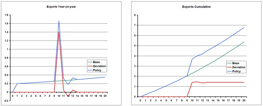
Figure 41.1 Little dynamic effect
For other variables, year-on-year results after year 10 might be quite different in base and policy runs. Strong dynamic mechanisms might produce such effects. For example, in Figure 41.2 we see that employment slowly returns to its base-run value after a year 10 increase. That implies that deviation year-on-year changes after year 10 have opposite sign to the year 10 effect.
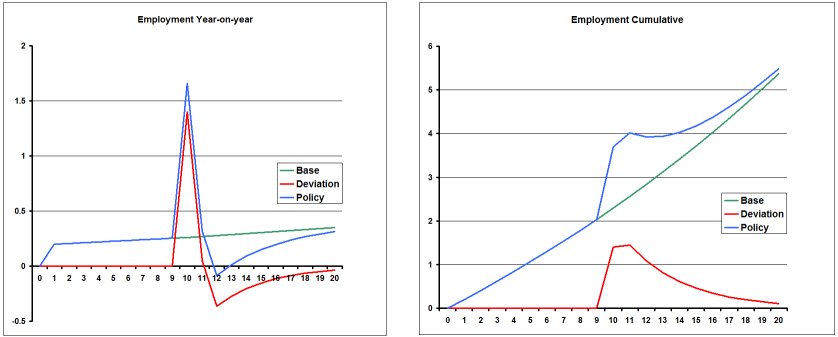
Figure 41.2 Pronounced dynamic effect
If we include subtotal statements for ALL shocks in base and policy, we should see that the sum of all subtotal effects on each year-on-year result (whether in base or in policy) is indeed equal to the total year-on-year result. However, the contributions of the common base shocks would be different in base and policy runs in year 10 and after. Thus, after subtracting base subtotals from policy subtotals to obtain subtotals contributions to deviation results, we would find that in year 10 some of the difference between base and policy runs was attributed to the base shocks; and that after year 10 ALL of the year-on-year differences between base and policy runs was attributed to the base shocks.
Hence, even though in reality the two year 10 policy shocks are the sole cause of differences between base and policy results, the subtotals method will attribute some of the difference to the base shocks which are common to both runs.
In Figure 41.1, the year-on-year effects of the year 10 policy shocks are mainly confined to year 10; after that, year-on-year changes are very similar in base and policy. Hence we would expect that the subtotals method would attribute nearly all of the cumulative difference between base and policy to the policy shocks.
By contrast, in Figure 41.2, the year-on-year effects of the year 10 policy shocks continue after year 10. Since there are no policy shocks after year 10, all of the year-on-year deviations after year 10 will be attributed to base shocks. The cumulative deviation at year 20 is near zero (employment has returned to control) — the subtotals method will attribute this to large positive contributions from the policy shocks, balanced by equal negative contributions from the base shocks. If employment is following a partial adjustment rule, we would likely find that among the base shocks, the main contributor to deviation results was the DelTime or DelUnity variable which is shocked to to simulate the passage of time.
41.3.4.1 Problem solved in a fully-intertemporal model [intertemsubtot]
A recursive-dynamic model can always be reformulated as a fully-intertemporal model (where all data and variables have an extra, time, subscript; and all periods are solved simultaneously). As in the recursive-dynamic model, all behaviour in the corresponding fully-intertemporal version would be based only on current and past variable values. The same base and policy results could be calculated using either recursive-dynamic or fully-intertemporal approaches (although the fully-intertemporal approach would likely be more demanding of computer resources). We'll assume that the starting point for the policy simulation is the all-periods updated database produced by the base simulation. In this case, the only shocks for the policy run will be the policy shocks, and the computed percentage change results will be the cumulative deviations from base.
Clearly the subtotals algorithm would attribute the causes of deviations more intuitively for this fully-intertemporal version. Since the only shocks for the policy run are the policy shocks, the whole of the cumulative deviation results will be exactly apportioned between effects of particular policy shocks. Note that, in the fully-intertemporal version, the subtotals algorithm tracks the effect of a particular shock in year 10, not only on year 10 variables, but also on each variable in each subsequent year. [In the recursive-dynamic version, changes in year N are attributed only to shocks in year N].
41.4 Suppressing arithmetic errors in ACCUM, DEVIA and CMBHAR [gpd5.10.3]
Normally, when the programs ACCUM, DEVIA or CMBHAR encounter an arithmetic problem (such as overflow — see section 34.3), they stop with a fatal error.
The most likely cause of overflow is having a percentage-change variable which should have been declared as a CHANGE variable in the TABLO Input file.
If you select option
ANF Arithmetic problems not fatal
in any of these programs, the program attempts to continue even if arithmetic problems occur. Instead you will see a warning. If an arithmetic problem occurs, or if a result goes outside what we consider to be a "safe" range, a somewhat arbitrary value will be given in the output file. In these cases, the programs attempt to signal the problem to you as follows.
- ACCUM adds "Arithmetic Problem" in the last column of the output spreadsheet file in every row for which an arithmetic problem was encountered.
- DEVIA does the same as ACCUM except that there is no space between "Arithmetic" and "Problem".
- CMBHAR adds the words "ARITH PROB" at the start of the long names of all arrays or variables for which an arithmetic problem was encountered.
RunDynam offers the option "Arithmetic problems not fatal for spreadsheet jobs" under the Run Preferences menu. When this option is selected, the windows programs runs ACCUM, DEVIA and CMBHAR with option ANF during the spreadsheet jobs.
42 Hands-on tutorials for models supplied with GEMPACK [gpd8.1]
Click here for detailed chapter contents
42.1 Overview of chapters 43 to 46 [gpd8.1b]
Section 1.2.2 suggested that beginning GEMPACK users should first work through the examples in the introductory chapters 3 to 7.
The following chapters 43 to 46 go on from those introductory chapters to provide more practice with GEMPACK. They give hands-on examples, with detailed instructions, for several of the economic models usually supplied with GEMPACK.
The examples in chapter 43 use WinGEM to manage models and simulations.
To learn about using the DOS prompt, work through the examples in chapter 44.
Chapter 45 contains an introduction to RunGEM, a Windows interface for carrying out simulations with models implemented via GEMPACK. Both new and experienced GEMPACK users may find that RunGEM helps them to carry out simulations easily and efficiently. RunGEM used in conjunction with TABmate can provide an alternative model development environment to WinGEM — see section 45.4. RunGEM provides an excellent environment for students to carry out simulations in a computer laboratory — see section 45.5.
Chapter 46 contains an introduction to AnalyseGE.
Section 60.1 lists the files associated with each model — these will usually be located in a subdirectory called EXAMPLES of the main GEMPACK directory (where GEMPACK files were installed on your computer). The instructions explain how to use these files to carry out particular simulations with the models. But we encourage you to try out your own different simulations. You can vary the closures or shocks, or the number of steps or solution method in multi-step simulations, and can also work with different condensations of the models.
When you start working with one of these models, we suggest that you create a new subdirectory for just this model (separate from the EXAMPLES subdirectory and from the directories containing the GEMPACK source and/or executable files); copy the relevant files from the examples subdirectory into it. (This avoids cluttering up the EXAMPLES directory and the directories containing the other GEMPACK files with model-specific files.)
43 Getting started with GEMPACK via WinGEM [gpd8.2]
Click here for detailed chapter contents
WinGEM is a GUI program used to control other GEMPACK programs, and to manage files created during simulations.
This chapter shows you how to use WinGEM and GEMPACK by giving you detailed instructions for carrying out various modelling tasks. The models used are some of the models described in chapter 42.
Work through the examples in this chapter to familiarise yourself with GEMPACK using WInGEM. Or, if you prefer to work at the Command (DOS) prompt, work through the examples in chapter 44.
We assume that you have GEMPACK (either either Source-code or Executable-image version) already installed on your PC — see section 2.
43.1 GEMPACK examples for new users [gpd8.2.1]
If you are a new user of GEMPACK, we recommend you first work through the Stylized Johansen examples in chapters 3 to 6. After completing those, work through the extra Stylized Johansen examples in sections 43.3.16 to 43.3.18. Then go on to the Miniature ORANI examples (section 43.4), or the GTAP examples (section 43.5) or the ORANIG examples (section 43.6) depending on your modelling interests.
You may also like to try using RunGEM for carrying out simulations with one of these models. A hands-on introduction to RunGEM is given in chapter 45.
43.2 Locating the example files [gpd8.2.2]
The examples below rely on files which are placed (at install time) in the Examples subdirectory of your GEMPACK directory (usually C:\GP\EXAMPLES). If you installed GEMPACK in a directory different from C:\GP, your Examples subdirectory will be the subdirectory EXAMPLES of the directory into which you installed GEMPACK.
43.2.1 Editing text files in WinGEM [gpd8.2.2.1]
We suggest you use TABmate as your text editor, as described in section 4.3.11. TABmate has coloured highlighting of TABLO syntax, and a powerful Gloss feature which displays all parts of the TABLO code where a chosen variable or coefficient is used. See section 4.3.2 for an example of using the Gloss feature.
43.3 Examples using the Stylized Johansen model SJ [gpd8.2.4]
Stylized Johansen is a small example general equilibrium model designed as an introductory teaching model (see Chapter 3 of Dixon et al (1992)). An introduction to this model is given in section 3.1.
The Stylized Johansen examples here are in two groups. The first group (sections 43.3.1 to 43.3.15) are compressed versions of examples covered in detail in chapters 3 to 6. The second group (sections 43.3.16 to 43.3.18) are not covered in detail elsewhere.
If you are a new user of GEMPACK, we encourage you to work through the versions in chapters 2 to 6 (rather than the compressed versions in sections 43.3.1 to 43.3.15 here). Then go on to sections 43.3.16 to 43.3.18 here.
43.3.1 Starting WinGEM [gpd8.2.4.1]
See section 3.4.1 for full details.
In Windows, double-click on the WinGEM icon to start the program.2 This should give the main WinGEM menu, as shown below, across the top of the screen.
WinGEM - GEMPACK for Windows
File Simulation HA Files Other tasks Programs Options Window Help
43.3.2 Preparing a directory for model SJ [gpd8.2.4.2]
See section 3.2 for full details about how to keep all example files for the Stylized Johansen model together in a separate directory C:\SJ and how to copy the relevant files into this directory.
All Stylized Johansen files start with the letters SJ to distinguish them from other files in the Examples directory.
Copy all the files SJ*.* in the Examples subdirectory of GEMPACK (usually C:\GP\EXAMPLES) to a working directory C:\SJ. There are about 20 such files.
43.3.3 Setting the working directory [gpd8.2.4.3]
WinGEM uses the idea of a working directory to simplify choosing files and running programs. It is important that you set the working directory before starting work on a model.
See section 3.4.2 for details about setting the working directory.
For the Stylized Johansen model examples here, the working directory needs to be the directory C:\SJ that you have just created and copied the files for Stylized Johansen into.
and select the directory C:\SJ.
43.3.4 Looking at the data directly using ViewHAR [gpd8.2.4.4]
The input-output data used in the Stylized Johansen model is contained in the data file SJ.HAR. Select from the main WinGEM menu :
The ViewHAR window will appear. Click on File | Open... and select the file SJ.HAR.
This will open the file SJ.HAR. See section 3.4.3 for details about what to look at in this file.
You can also look at the data in a Header Array file using the GEMPACK program SEEHAR as described in section 43.3.17 below.
43.3.5 TABLO-generated program or GEMSIM? [gpd8.2.4.5]
As described in section 3.5.1, there are two ways of running a simulation using either the TABLO-generated program or the GEMPACK program GEMSIM. The steps using a TABLO-generated program are in section 43.3.6 below. There we assume that you have a Source-code version of GEMPACK and that an appropriate Fortran compiler is on your DOS PATH.
Alternatively, you could also use the GEMSIM method (as in section 43.3.7 below).
If you don't have the Source-code version (ie, you have an Executable-image version of GEMPACK), you must use GEMSIM — see section 43.3.7.
The simulation results are the same whether you use GEMSIM or the TABLO-generated program for the model.
43.3.6 The example simulation using a TABLO-generated program [gpd8.2.4.6]
See section 3.5.2 for full details of running a simulation using a TABLO-generated program.
The three steps involved in carrying out a simulation using GEMPACK are:
- Step 1 — Implement the model
- Step 2 — Solve the equations of the model
- Step 3 — View the results
43.3.6.1 Step 1 — Implementing the model SJ using TABLO [gpd8.2.4.6.1]
The TABLO Input file is called SJ.TAB. It contains the theory of the Stylized Johansen model. From WinGEM choose3
Click on the Select button to select the name of the TABLO Input file SJ.TAB. Click on the Edit button to view this file in your editor.
At top right of the TABLO window, ensure that Fortran (not GEMSIM) is selected.
In the TABLO window, click on the Run button to run TABLO.
Click on the Go to Compile and Link button at the bottom of the TABLO window to run the Fortran compiler.
Click on the button Compile and Link and wait while the compiler converts the Fortran file SJ.FOR into the executable image SJ.EXE.
When finished, click on the button Go to 'Run TG Program'
43.3.6.2 Step 2 — Solve the equations of the model [gpd8.2.4.6.2]
The Command file SJLB.CMF contains a closure with supplies of the two factors, labor and capital, as exogenous variables. The shock increases the supply of labor by 10 percent and holds the supply of capital fixed.
Select the Command file called SJLB.CMF.
Click on Run to run SJ.EXE with the Command file SJLB.CMF.
43.3.6.3 Step 3 — Look at the results with ViewSOL [gpd8.2.4.6.3]
Click on the button Go to ViewSOL to open the Solution file SJLB.SL4 created at the previous step.
In the Contents list, to see the results of one of these variables, just double-click on the corresponding row in the Contents list. To check results of the simulation, double-click on the p_XCOM row. Then you should see something like the following:
| p_XCOM | sjlb | Pre sjlb | Post sjlb | Chng sjlb |
| s1 | 5.885 | 8.000 | 8.471 | 0.471 |
| s2 | 6.899 | 12.000 | 12.828 | 0.828 |
43.3.7 The example simulation using GEMSIM [gpd8.2.4.7]
See section 3.5.3 for full details of running a simulation using GEMSIM.
Carry out the three steps of a simulation :
Step 1 — Implement the model
Step 2 — Solve the equations of the model
Step 3 — Look at the results
43.3.7.1 Step 1 — Implementing the model SJ using TABLO [gpd8.2.4.7.1]
The TABLO Input file is called SJ.TAB. It contains the theory of the Stylized Johansen model. Choose:4
Click on the Select button to select the name of the TABLO Input file SJ.TAB. Click on the Edit button to view this file in your editor.
At top right of the TABLO window, ensure that GEMSIM (not Fortran) is selected.
In the TABLO window, click on the Run button to run TABLO.
Click on the Go to GEMSIM button at the bottom of the TABLO window.
43.3.7.2 Step 2 — Solve the equations of the model [gpd8.2.4.7.2]
As an example of a simulation, the Command file SJLB.CMF contains a closure with supplies of the two factors, labor and capital, as exogenous variables. The shock increases the supply of labor by 10 percent and holds the supply of capital fixed.
Select the Command file called SJLB.CMF.
click on Run to run GEMSIM with the Command file SJLB.CMF.
43.3.7.3 Step 3 — Look at the results with ViewSOL [gpd8.2.4.7.3]
Click on the button Go to ViewSOL to open the Solution file SJLB.SL4 created at the previous step.
In the Contents list, to see the results of one of these variables, just double-click on the corresponding row in the Contents list. To check results of the simulation, double-click on the p_XCOM row. Then you should see something like the following:
| p_XCOM | sjlb | Pre sjlb | Post sjlb | Chng sjlb |
| s1 | 5.885 | 8.000 | 8.471 | 0.471 |
| s2 | 6.899 | 12.000 | 12.828 | 0.828 |
43.3.8 Source-code version : use GEMSIM or TABLO-generated program? [gpd8.2.4.8]
Readers with Source-code GEMPACK have the choice of using GEMSIM or the TABLO-generated program. (If you have the Executable-image version you must use GEMSIM.)
For small models such as Stylized Johansen (section 43.3 here), Miniature ORANI (see section 43.4 below) or 3-region, 3-commodity GTAP (see section 43.5), GEMSIM is quite fast. TABLO-generated programs only show their great advantage with large models and/or more disaggregated data sets (see chapter 72).
43.3.9 The updated data — another result of the simulation [gpd8.2.4.9]
See section 3.9 for full details about looking at the updated data in file SJLB.UPD.
Select from the main WinGEM menu,
Click on File | Open and open the file SJLB.UPD.
43.3.10 Several Johansen simulations [gpd8.2.4.10]
See chapter 58 for full details about using SAGEM to carry out Johansen simulations.
The starting point is always the Equations file for the model which is produced by running the TABLO-generated program SJ.EXE or GEMSIM.
43.3.10.1 Preparing an Equations file for use by SAGEM [gpd8.2.4.10.1]
An Equations file for Stylized Johansen can be created by running the TABLO-generated program SJ.EXE or GEMSIM and taking inputs from the Command file SJEQ.CMF.
In the main WinGEM menu, select Simulation. Then select either GEMSIM Solve (or alternatively select RunTGProgram and select the TG Executable SJ.EXE)5.
Select the Command file SJEQ.CMF and Run the simulation.
43.3.10.2 Carrying out the Johansen simulations with SAGEM [gpd8.2.4.10.2]
You will use the Command file SJLBJ.CMF for running SAGEM to carry out these simulations. This gives shocks of 1 percent to supplies of both labor and capital.
Click on Simulation | SAGEM Johansen Solve... in the main WinGEM window.
Select the file SJLBJ.CMF.
To run this Johansen simulation, Run the program SAGEM.
Click on the button Go to ViewSOL to open the Solution file SJLBJ.SL4.
43.3.11 Changing the closure and shocks [gpd8.2.4.11]
Several simulations can be carried out on the same model by changing the closure and/or the shocks in the Command file. The example in section 3.11 shows you how to make a new Command file in the text editor and then run another simulation using SJ.EXE (or alternatively GEMSIM). The simulation is to increase the price of labor by 3 per cent and to increase the supply of capital, by 10 per cent. In order to increase the price of labor, the variable p_PF("labor") needs to be exogenous so you need to change the closure, and also, apply different shocks.
You should work through the hands-on example in section 3.11.
43.3.12 Correcting errors in TABLO input files [gpd8.2.4.12]
When you build your own model, you will need to correct errors in your TABLO Input file. In the examples below, we show you how to do this with a version of SJ.TAB which has a couple of the sorts of errors that all modellers make.
A detailed example is given in section 4.7.1.
To begin, use File | Edit file... to open the file SJERROR.TAB.
Now please check how your WinGEM is configured by selecting
Now open a TABLO window via Simulation | TABLO Implement... and then, in this window, Select this TABLO Input file SJERROR.TAB. Click on Run to run TABLO. Of course this run will find errors and so you will see a new window titled Error running TABLO. In this window, click on Edit TABLO file.
This will put you into the windows program TABmate which will open with this TABLO Input file SJERROR.TAB. Further details are given in the corresponding example in section 4.7.1.
The procedure for removing errors from TABLO Input files is: Run TABLO, use TABmate (and its TABLO Check button) to remove all errors, then close TABmate, click on Rerun to rerun TABLO under WinGEM to produce a TABLO-generated program or output for GEMSIM.
As we indicated above, WinGEM provides different ways of proceeding when a syntax or semantic error is discovered in the Check stage of TABLO. The example above shows the usual way of proceeding using TABmate, which is the way we recommend for new users. Below we show you a different way of proceeding. If you are a beginner, we strongly suggest that you skip this alternative and come back to it when you are more familiar with WinGEM and GEMPACK. We only include it here for completeness.
43.3.12.1 Correcting errors in SJERROR.TAB via WinGEM and Split Window Editing [gpd8.2.4.12.1]
Begin by using File | Edit file... to open the file SJERROR.TAB. Then use Save As... to change the name to SJ3.TAB and then exit from the editor. [We ask you to do this so that the file SJERROR.TAB remains as it is for others to access on your machine.]
Now please configure your WinGEM to use split-screen editing after a TABLO Check error by selecting
and then slide your mouse across to click on Use GemEdit (Split Window).
Now, open a TABLO window via Simulation | TABLO Implement... and then, in this window, Select this TABLO Input file SJ3.TAB. Click on Run to run TABLO. Of course this run will find errors and so you will see a new window titled Error running TABLO. In this window, click on Edit TABLO file.
Now you see the difference between this example and the one above. This time you are put into a GemEdit window in which the TABLO file SJ3.TAB is in the top part and the Information file SJ3.INF is in the bottom part. And the cursor is positioned in SJ3.TAB at the place where the first error is found.
You should see that the cursor is positioned at the start of the third of the three lines shown below.
VARIABLE (all,f,FAC) PF(f) # Price of factor f #
! This is p:i (i=3,4) in DPPW !
VARIABLE (all,i,SECT) XCOM(i)
The first two lines are the declaration of VARIABLE PF(f) and the third line is meant to be the start of the declaration of VARIABLE XCOM(i). But we have left out the semicolon required at the end of the second of these three lines (a very common error in TABLO Input files). So you should correct this error by adding a semicolon ; at the end of the second of these three lines in the top part of the screen.
Now click on Next error to go to the next error. You will see that the cursor is now pointing in the top part of the screen to just before the "FACT" in the line below.
COEFFICIENT (all,f,FACT)(all,j,SECT) ALPHAFAC(f,j)
In the Information file in the bottom part of the screen, the error is recorded as
87 COEFFICIENT (all,f,FACT)(all,j,SECT) ALPHAFAC(f,j)
?
%% Semantic problem
Unknown set.
The ? points just below "FACT" suggesting that this is where the error is. Indeed, this error has occurred because the set FAC has been incorrectly spelled (another common error) as FACT (with an extra T). Correct this error by deleting (in the top half of the screen) the extra T.
Now click on Next error to go to the next error. You will see, in the Information file
109 FORMULA (all,i,FAC) PF(i) = 1.0 ;
?
%% Semantic problem.. Unknown coefficient or variable.
The ? is pointing to PF and the message indicates that this is an unknown coefficient or variable. We know that this error is a consequence of the first error since a semicolon was omitted at the end of the declaration of this variable. You have already fixed that earlier error and there is nothing else to correct here. If you continue looking at the remaining errors you will see that they are all consequences of the first two errors which are now corrected. Thus you should use File | Exit to exit from SJ3.TAB, saving the changes. Then close the error window by clicking on Close.
This should put you back to the TABLO window where you can click on Run to run TABLO again with the modified SJ3.TAB file. Hopefully this time you will find no errors.
This illustrates the procedure for removing errors from TABLO Input files using Split Window editing with GemEdit. Run TABLO, use split window editing to remove some errors and then rerun TABLO until all errors are eliminated. As indicated above, we think that most users will find the TABmate alternative the most efficient way of eliminating errors.
43.3.13 Creating the base data header array file [gpd8.2.4.13]
Making a data file for Stylized Johansen using ViewHAR is discussed in section 6.1. You should work through the hands-on examples there.
[Full details on using the program MODHAR to create or modify data files are given in chapter 54.]
43.3.14 Modifying data on a header array file [gpd8.2.4.14]
The program ViewHAR is used to modify data on a Header Array file. See section 6.2 for hands-on examples you can work through.
43.3.15 Condensing the model [gpd8.2.4.15]
When large models are implemented, it is usually necessary to condense the model. This means carrying out algebraic substitutions to reduce the size of the system of linear equations solved at each step of a multi-step calculation. The concept of condensation is discussed in section 14.1.
See section 3.8.2 and 14.1.4 for hands-on examples showing you
- how to make a condensation Stored-input file for Stylized Johansen, and
- how to run TABLO using a condensation Stored-input file.
43.3.16 Transferring simulation results to a spreadsheet using SLTOHT [gpd8.2.4.16]
The program SLTOHT is used to convert results on a Solution file to either a Header Array file or a text file in CSV format (Comma Separated Values) suitable for importing the results into a spreadsheet program such as Excel. A spreadsheet program will usually place the values of an array separated by commas into separate cells in the spreadsheet.
See the examples in section 3.10 for details about running SLTOHT with the option SSS and SSE. Both examples use Spreadsheet Mapping files.
In the example below you will convert the results from the file SJLBJ.SL4 created in section 43.3.10 to a text file in CSV format where the numbers in the array are separated by commas. This example does not use a Spreadsheet Mapping file.
Note that SJLBJ.SL4 is produced by running SAGEM. This Solution file contains the totals (cumulative) column of results and two individual column results. You will see all three solutions on the spreadsheet file produced in the example below.
43.3.16.1 Example — Running SLTOHT without using a Spreadsheet Mapping file [gpd8.2.4.16.1]
Select from the WinGEM menu
In the SLTOHT window, select from the menu,
Options | SLTOHT Options
A screen of SLTOHT option choices will appear. Click on
and select a Comma as separator. (A comma is the default choice.)
Select to output all Solutions on the Solution file. Click on Ok to accept these options and return to the main SLTOHT screen.
Click on the Select and choose the Solution file SJLBJ.SL4. Choose to print All solutions. Click the Ok button.
Run the program SLTOHT. This will create the CSV text file called SJLBJ.CSV. When the program has completed, View the text file.
Look first at the p_XCOM results which are shown as follows:
! Variable p_XCOM # Total demand for (or supply of) commodity i # ! Showing this as an array of size 2x3 ! Solutions in columns -- each row is a different component 2,3, real spreadsheet; 0.60000002 , 0.40000001 , 1.0000000 , 0.69999999 , 0.30000001 , 1.0000000 ,
What do all these numbers represent? This is explained near the top of the file SJLBJ.CSV where you see
! For each variable below columns represent the following solutions: ! 2 INDIVIDUAL column(s) each one giving the solution ! for an individual shock. ! 1 TOTALS column giving cumulative solutions across ALL shocks.
This reminds you of the solutions you see on the file SJLBJ.CSV and tells you how they are set out on the file. Each column is a different solution and each row is a component of a variable.
Look again at the p_XCOM results. The first row of numbers is for the first component p_XCOM("s1"). The first number 0.60000002 in that row is the first individual column result (the effect of just a 1 percent increase in the supply of labor). The second number 0.4000001 is the second individual column result (the effect of just a 1 percent increase in the supply of capital). The third number (1.0) is the totals solution (which shows the combined effect of 1 percent increases in the supplies of both labor and capital).. The "2 3 spreadsheet ;" line is the "how much data" information (see chapter 38) for this array of data on the GEMPACK text data file SJLBJ.CSV.
Now look at results for the other variables.
You can also try starting your spreadsheet program (for example Excel) and opening the file SJLBJ.CSV (as a text file with commas for separators). Look at the arrays of results (ignoring rows that start with an exclamation mark which are comments).
There are various other ways of running the program SLTOHT, for example by using a Spreadsheet Mapping file as described in chapters 8 and 40.
43.3.17 Using SEEHAR to look at data [gpd8.2.4.17]
You may want to print out the data in the data files of a model. The program SEEHAR can be used to prepare a print file of all the data on a Header Array file.
In the WinGEM main menu, select
Click on the Select button and choose the file SJ.HAR.
Click on the Run button to run the program SeeHAR. When this has completed, click on the View file button to see the Print File SJ.SEE. The file SJ.SEE is a text file which could be printed out on a printer. (If an error occurs, you can use the View Log file button to see what has happened.)
Find the data at header CINP in this file, which should look like the box shown below.
Page 1 of Display of (all of) 'DVCOMIN(SECT,SECT)'. This coefficient is of size 2x2. (This data is at header 'CINP' on the file. Long name is 'Intermediate inputs of commodities to industries - dollar values'.) ---------------------------------------------------------------- Next submatrix contains numbers from DVCOMIN(SECT,SECT) part, which are positions (1-2, 1-2) of DVCOMIN(SECT,SECT). COLUMN 1 2 ROW ROW TOTALS No. Name s1 s2 1 s1 4.000000 2.000000 6.000000 2 s2 2.000000 6.000000 8.000000 COLUMN TOTALS 6.000000 8.000000 14.000000
DVCOMIN is the name used for this data in the TABLO Input file for the Stylized Johansen model.
The actual data in the file at this header is just the 2x2 matrix. SeeHAR calculates and shows the row and column totals.
Use the Page Down key to find the DVFACIN data at Header FINP and find out how much Labor is used by Sector s2.
Click on File | Exit to exit from the editor, and again on File | Exit to exit from the SeeHAR window.
43.3.18 Analysing simulation results using AnalyseGE [gpd8.2.4.18]
You can find a hands-on introduction to analysing simulation results using AnalyseGE in section 46.1. This example analyses the results of the 10 percent labor increase in Stylized Johansen.
We encourage you to work through this example.
43.3.19 What next ? [gpd8.2.4.19]
This completes the Stylized Johansen examples. We suggest that you exit from WinGEM (which will close all WinGEM Windows also).
You may wish to continue learning about WinGEM by working with one of the other models in chapter 42.
Alternatively, you may like to try using RunGEM to carry out simulations with Stylized Johansen; if so, a hands-on introduction is given in section 45.1 below.
43.4 Miniature ORANI model examples [gpd8.2.5]
The following examples are based on the Miniature ORANI model MO. This is a pedagogical model designed to introduce some of the essential ideas behind the ORANI model of the Australian economy -- see sections 3-9 of Dixon et al. (1982).
43.4.1 Preparing a directory for model MO [gpd8.2.5.1]
To keep all examples files for this model together in one area, create a separate directory \MO and copy all MO*.* files in you examples directory (usually C:\GP\EXAMPLES) to this subdirectory. You can use Windows Explorer or DOS commands as in the examples for Stylized Johansen (see section 43.3.2 above). In DOS, use the commands (the third of which you will need to change if your examples directory is not C:\GP\EXAMPLES):
md \mo cd \mo copy c:\gp\examples\mo*.* dir
43.4.2 Set the working directory [gpd8.2.5.2]
First set the working directory to be this directory \MO by choosing
and select the directory MO on the appropriate drive. [See section 43.3.3 above for more details.]
Examine the TABLO Input file MO.TAB in your text editor (preferably TABmate — see section 43.2.1) to see the theory of the Miniature ORANI model — the variables used, the data read in, and the equations to be solved. Choose
File | Edit file... and open the file MO.TAB.
43.4.3 Examine the database for MO [gpd8.2.5.3]
The data for this model is in the file MO.DAT. Since this is a Header Array file use ViewHAR to look at the arrays of data which it contains. Choose
as you did with the data file for Stylized Johansen (see section 43.3.4).
43.4.4 Implementing the model MO using TABLO [gpd8.2.5.4]
As in Step 1 in section 43.3.6 or 43.3.7, open a TABLO window
Select the TABLO Input file MO.TAB and then Run TABLO. If you have a Source-code version and produced a TABLO-generated program, click
to create the Executable image of the TG program MO.EXE.
When the model has been implemented successfully, select .Go to Run TG program (or Go to GEMSIM) to go on to the simulation (Step 2).
43.4.5 Simulation using the command file MOTAR.CMF [gpd8.2.5.5]
Select the Command file MOTAR.CMF and Edit the file.
Examine the closure and shocks applied in the simulation. Exit from the editor and then Run MO.EXE (or GEMSIM) to solve the equations.
Then proceed as in Step 3 in section 43.3.6 or 43.3.7 above to look at the results. That is, click on Go to ViewSOL to look at the results via ViewSOL.
The simulation is a multi-step 2-step, 4-step, 6-step using the Gragg method followed by extrapolation.
To estimate the accuracy of this solution an Extrapolation Accuracy file called MOTAR.XAC is produced. [Extrapolation Accuracy files are discussed in section 3.12.3 and in section 26.2.3.]. Choose
in the main WinGEM menu and examine MOTAR.XAC in the text editor. This shows the results for each endogenous component of each endogenous variable. The first column contains the results for a 2-step solution, the second for a 4-step one, the third for a 6-step and the fourth column contains the extrapolated solution which is an accurate solution of the non-linear model. See section 26.2.3 for information about the component numbers and the codes (for example, "CX") shown on the file.
Also look at the Extrapolation Accuracy Summaries for the variables and data (see sections 26.2.1 and 26.2.2 respectively). You can find these near the end of the Log file MOTAR.LOG.
43.4.6 Several Johansen simulations using SAGEM [gpd8.2.5.6]
In the editor (use File | Edit file from WinGEM's main menu), look at the Command file MOSAGEM.CMF (usually supplied with GEMPACK). Check that MOSAGEM.CMF contains the text below:
Command file MOSAGEM.CMF use equations file mo ; use environment file mo ; ! Name of Solution file is inferred from name of Command file. ! (See section 20.5.) ! Choosing sets of variables individually-retained exogenous %all ; individually-retained endogenous p_Z p_YCOMIND(COM,"i2") p_XINTFAC 1-3 %macro ; cumulatively-retained endogenous p_Z p_YCOMIND (COM) (FAC,IND) ; ! Shocks shock P_T 2 = 1 ; shock p_phi = 1 ; shock p_fwage = -2.38 ; shock p_cR = 2.76 ; ! Subtotals results subtotal p_T = tariff shock ; subtotal p_PHI = exchange rate shock ; subtotal p_FWAGE p_CR = wage and real consumption shocks ; verbal description = MO standard closure ;
Then run SAGEM with the file MOSAGEM.CMF by selecting
This should produce a Solution file MOSAGEM.SL4.. [The name is derived from the name of the Command file as explained in section 20.5.]
The Solution file MOSAGEM.SL4 produced by this run of SAGEM contains
- the cumulative solution (the effect of all shocks),
- four individual column results (one for each component shocked), and
- three subtotals results (one for each "subtotal" statement in the Command file).
[See 58.1 and 58.2 for information about these different types of solutions, and see section 66.5.1 for information about the "choosing sets" statements in the Command file.]
43.4.6.1 Looking at the Results [mosagemresults]
Click on Go to ViewSOL.
To make sure you are seeing all the results in ViewSOL,
click on menu item File | Options.
In the Options form, make sure that items
Show subtotal results (if present)
and
Show individual column results (if present)
are selected. [Click on them if not.]
Then click OK. Then close ViewSOL and run it again.
In the "which solution" drop-down menu, you should see 8 items.
- The first is labelled "mosagem". This refers to the cumulative solution.
- Columns 2 to 4 are labelled "tariff shock", "Subtotal 2" and "Subtotal 3". These refer to the three subtotals results. [Notice that ViewSOL shows the subtotal description from the Command file MOSAGEM.CMF for the first subtotal since "tariff shock" is short, but it shows "Subtotal 2" because the subtotal description there "exchange rate shock" is longer.]
- Columns 5 to 8 are labelled "p_T(2)", p_FWAGE(1)", "p_CR(1)" and "p_PHI(1)" respectively. These refer to the individual column results. [The numbers in brackets are component numbers. For example, the p_T shock is to component number 2 of p_T, while the shock to p_CR is to component 1 (the only component) of p_CR.]
Now look at the results.
For example, click on "Macros" in the ViewSOL Contents page. You should see the cumulative solution (under the heading "mosagem"), then the three subtotals results for these variables, and finally the 4 individual column solutions for these variables. Since the macro variables shown here all happen to be exogenous in this simulation, what you see are the values of the shocks.
Now, to see results for the endogenous variable p_Z (industry activity), click on menu item Contents and then click on the "p_Z" row in the Contents page. You will see the endogenous results for p_Z in the 8 different columns. For example, for sector "i1",
- the "tariff shock" subtotal result is -0.444 which is the same as the "p_T(2)" individual column result.
- the "Subtotal 3" result is 3.588 which is the sum of the "p_FWAGE(1)" and "p_CR(1)" individual column results. That is because Subtotal 3 contains the effect of those two shocks (see the Command file MOSAGEM.CMF).
Now look at results for the 2-dimensional variable p_PFAC by clicking on Contents and then clicking on "p_PFAC" in the Contents page. What you see depends on the solution indicated in the "Which solution" drop-down box. For example, to see the individual column results for the shock to p_CR, you need to select solution "p_CR(1)".
Close ViewSOL and the SAGEM window in WinGEM.
43.4.7 Homogeneity test using SAGEM [gpd8.2.5.7]
To test whether models are homogeneous in price, you can shock nominal variables by 1 percent and leave all quantity variables unshocked. (See section 79.1 for more information.) This example carries out one such homogeneity test for model MO.
Copy the Command file MOSAGEM.CMF to a new file MOHOMOG.CMF and edit MOHOMOG.CMF so that only the exchange rate p_phi is shocked and the shock is 1 percent. Remove the subtotals statements.
Change the name of the Solution file to MOHOMOG but use the same Equations file and Environment file (MO). Rerun the simulation using SAGEM as in the previous example. [If there is an error, see section 4.7.2 for advice about identifying and fixing the error.]
Run ViewSOL to look at the results. If the model MO is homogeneous, all nominal variables should have increased by 1 percent and all quantity variables should be zero.
43.4.8 Modifying the closure for MO [gpd8.2.5.8]
To modify the closure in the Command file MOTAR.CMF, first copy it to a new file name MOTAR2.CMF, then edit it to make the following changes:
(1) Replace the exogenous variable p_phi by the variable p_cpi
(2) Replace the second component of p_XEXP, p_XEXP("c2") in the exogenous list . by the second component of p_V, p_V("c2")
(3) Change the name of the Environment file from MO to MO2.
(4) Change the verbal description at the end to indicate these changes have been made.
Run a simulation using MO.EXE (or GEMSIM) and this new Command file MOTAR2.CMF. [If you encounter an error running the simulation, see section 4.7.2 for advice about identifying and fixing the errors in your Command file.]
Look at the results via ViewSOL to see the effect of this closure swap.
43.5 Examples for global trade analysis Project model GTAP94 [gpd8.2.6]
The following examples are for the multi-regional model, GTAP94, described in Hertel (1997). Several different aggregations (of commodities and/or regions) are available from the Project. See also section 43.6 for examples using the more recent version GTAP61.TAB of this model.
Preparing a Directory for Model GTAP94
To keep all examples files for this model together in one area, create a separate directory \GTAP and copy all G*.* files from your examples directory (usually C:\GP\EXAMPLES) to this subdirectory. You can use File Manager or DOS commands as in the examples for Stylized Johansen (see section 43.3.2 above). In DOS, use the commands (you will need to alter the third one if your examples directory is not C:\GP\EXAMPLES):
md \gtap cd \gtap copy c:\gp\examples\g*.* dir
In WinGEM, first set the working directory to be this directory \GTAP by choosing
and select the directory GTAP on the appropriate drive. [See section 43.3.3 above for more details.]
43.5.1 Examining the GTAP data directly [gpd8.2.6.1]
There are three data files associated with each GTAP data set. For the 3x3 aggregation, the files are
| GDAT2-01.HAR | The Global data set (I/O for each region, trade data etc) |
| GSET2-01.HAR | Set information, giving region and commodity names in aggregation |
| GPAR2-01.DAT | Parameter values |
There are also three data files for a 10x10 aggregation:.
GDAT2-06.HAR, GSET2-06.HAR and GPAR2-06.DAT.
Using ViewHAR to view the global data for the 3x3 aggregation
The GTAP global data file contains large amounts of data including the input-output data for each region and trade data.
This file is given the (logical) name GTAPDATA in the TABLO Input file GTAP3x3.TAB which lays down the theory of GTAP. To see what information is on this global data file, select
The Open box should list several files associated with the GTAP model. Under the Edit File menu item, the type of files you can edit are all text (ASCII) files. (The editor you are using is called GEMEDIT which automatically saves files as text files.)
Select the TABLO Input file to edit:
GTAP3x3.TAB
Then search for GTAPDATA. [To search in GEMEDIT, select Search | Find... from GEMEDIT's menu, then type in the word(s) you wish to search for, and finally type a carriage return. Use this technique to search for GTAPDATA. To search again after you have found the first occurrence of "GTAPDATA", you can either select Search | Search again from GEMEDIT's main menu or you can touch the F3 key (near the top of your keyboard).. Use this technique to see the first 3-4 occurrences of GTAPDATA.]
You will see that various pieces of data are read from this file.
One of these is the array VDPA(i,r) whose values are held at header "VDPA". To see this and to find out what data is stored at this header and associated with VDPA(i,r) in GTAP3X3.TAB, move to the start of GTAP3X3.TAB (use Ctrl+Home, that is, hold down the Ctrl key and touch the Home key). Then search for VDPA. You will see that VDPA(i,r) is declared as a COEFFICIENT and that it holds the data for "Value of Private household expenditure on Domestic commodity i in region r, valued at Agents' prices".
By searching again for VDPA you will see that this data is read from file GTAPDATA at header "VDPA".
Exit from GEMEDIT in the usual Windows way by File | Exit. (There are usually alternatives in terms of keystrokes instead of the mouse action. For example you can use keystrokes Alt followed by f followed by x in order to exit.)
To see the VDPA data in the 3x3 aggregation, you can run the program ViewHAR. To do this, select HA files | View VIEWHAR from WinGEM's main menu.
A ViewHAR window will appear. Click on
and open the file GDAT2-01.HAR in directory \GTAP.
This will open the file GDAT2-01.HAR and show its contents on the Contents screen.
Each of the rows corresponds to a different array of data on the file. Look at the column under the heading Name to see what these arrays are.
| Header | Type | Size | Name | |
| 1 | EVFA | RE | ENDW_COMMxPRO | Endowments - Firms' Purchases at Agents' Prices |
| 2 | EVOA | RE | ENDW_COMMxREG | Endowments - Output at Agents Prices |
| (etc) | ||||
| 9 | VDPA | RE | TRAD_COMMxREG | Intermediates - Household Domestic Purchases ... |
| (etc) |
You can see that array number 9 is the data at Header "VDPA". The data at this header is the value of households' domestic purchases at agents' prices. To see the actual data, double-click on the VDPA row. What is the value of EU households' domestic purchases of manufactures at agents' prices? What about purchases of food by households in ROW (that is, Rest of the World)?
Now click on Contents in the ViewHAR window showing the data and you will return to the list of contents of the arrays in this global data file. Look at the VDFM row (array number 6). You can see that the associated data is a 3-dimensional array of size TRAD_COMM x PROD_COMM x REG and that this is described as "Intermediates - Firms' Domestic Purchases at Market Prices".
(Note that the sizes of the sets in this GTAP aggregation GTAP3x3 are
Set TRAD_COMM 3 elements, Set PROD_COMM 4 elements, Set REG 3 elements
so the array VDFM is of size 3 x 4 x 3.)
To see the actual data, double-click on this VDFM row. You see a 3x4 matrix of data (plus a totals row and a totals column) with the rows labelled "food", "mnfcs" and "svces" and the columns labelled "food", "mnfcs", "svces" and "CGDS". These must be the elements of the sets TRAD_COMM (tradeable commodities) and PROD_COMM (produced commodities) respectively. What about the 3rd dimension REG of this data? The clue is given by the 3 drop-down lists near the top right-hand corner of the screen which say
All TRAD_COMM All PROD_COMM Sum REG
respectively. Because your computer screen is 2-dimensional, what you are seeing are the VDFM values summed across regions (REG). What is the total across all regions of the value at market prices of domestic purchases of services by the food firms? What about of manufactures by the capital-goods firms?
How can we see the value of firms' purchases in just one region, for example in EU? To see this, click on the Sum REG drop-down list box near the top right-hand side and select EU from the options. The data will change and now you are seeing how much is purchased just by firms in the EU. What is the value at market prices of purchases of services by manufacturing firms in the EU? What about by manufacturing firms in the USA?
There are lots of ways of viewing 2-dimensional slices of a 3-dimensional array. To see another, click on the TRAD_COMM drop-down list box (the first of the three) and select Sum TRAD_COMM. Now click on the REG list box and select All REG. What does the number in row "food" and column "ROW" indicate? What is the total value (at market prices) of all intermediate inputs into the services sector in the EU?
What is the value at market prices of intermediate inputs of manufactures to the capital goods sector in "ROW"? [There are various ways you can see this. One is to select "ROW" in the REG list box. Another is to select "CGDS" in the PROD_COMM list box.]
Recall that you are looking at the TRAD_COMMxPROD_COMMxREG data at header "VDFM" in the global data set. To check what data is read from this header according to the description of the model in GTAP3X3.TAB, find the WinGEM main menu on your screen, select File | Edit file... and open file GTAP3X3.TAB. Search in it for VDFM until you find the lines saying which data is read from this header (it is the values of Coefficient VDFM(i,j,r) where i is the tradeable commodity, j is the produced commodity (firm) and r is the region). Return to the top of the file (use Ctrl+Home) and then search again for VDFM. You will see indeed that VDFM(i,j,r) is described as "purchases of domestic i r for use in j in region r". Now close GTAP3X3.TAB via File | Exit.
Also close the ViewHAR window by selecting File | Exit from ViewHAR's (not WinGEM's) menu.
.Using ViewHAR to view the set information
The set information tells which regions and commodities are represented in the current aggregation of the data. This set information file is given the (logical) name GTAPSETS in the TABLO Input file GTAP3X3.TAB which lays down the theory of GTAP. To see what information is on this set information file, select File | Edit file... and open GTAP3X3.TAB.
Then search for GTAPSETS. You will see that
the names of the regions (the SET of regions is called REG) are held at header "H1",
the names of the tradeable commodities (the SET is called TRAD_COMM) are held at header "H2", and
there are several other SETs defined.
Leave this file open in the editor GEMEDIT. (It will be convenient to return to it later.)
The GTAPSETS data file for the 3x3 aggregation is called GSET2-01.HAR. To see the actual data at these headers in this file, you need to return to WinGEM by clicking on the WinGEM taskbar at the top of the screen. Then click on
HA files | View VIEWHAR in WinGEM's main menu and open GSET2-01.HAR. The Contents list begins
| Header | Type | Size | Name | |
| 1 | H1 | 1C | 3 length 12 | |
| 2 | H2 | 1C | 3 length 8 |
The data type "1C" means character data (i.e., lists of names). The "3 length 12" means that there are 3 names of (maximum) length 12 held at header "H1".
To look at the names at header "H1", double-click on this row in the Contents. What are the 3 regions called? Return to the Contents (click on Contents) and look at the data at header "H2". As you know from GTAP3X3.TAB (look at it again if you are not sure — it is still open at the right place) these are the names of the 3 tradeable commodities.
Close this ViewHAR window by selecting File | Exit from ViewHAR's menu. [But leave GTAP3X3.TAB still open in GEMEDIT.]
Using SeeHAR to look at the global data
In the first GTAP example you used ViewHAR to look at different parts of the data in the global data set GDAT2-01.HAR. This is an excellent way of looking at individual items of data; indeed you can use ViewHAR's print features to print out selected 2-dimensional slices of some of the arrays. But sometimes you will want to print out the whole data base or at least several of the arrays. Then it may be best to use the program SEEHAR.
To see how SeeHAR works, select
from WinGEM's main menu. [Use the Taskbar or Alt+Tab if necessary to switch to WinGEM.]
A SeeHAR task window appears in the middle of your screen.
Click on the Select button (WinGEM has marked this as the obvious thing to do by putting dots around the text on this button).
In the file open dialogue box which appears, select the global data file GDAT2-01.HAR (which you can do either by double-clicking on this name in the list of files or by single-clicking on it and then selecting Ok).
Now the Run button is marked as the obvious thing to do so click on it. A DOS box appears and WinGEM has started the program SeeHAR running to examine the data on this file. When it finishes running (it will take less than a minute), take WinGEM's advice and click on View file.
Search for VDPA which is the header whose data you looked at via ViewHAR earlier. You will see that at header "VDPA" is 3x3 data described as "Intermediates - Household Domestic Pur" [the name is truncated] and denoted by VDPA(TRAD_COMM,REG) which means it is 2-dimensional data, the first argument being in TRAD_COMM and the second in REG. Repeat the search for VDPA until you see the actual data. It is shown as a 3x3 matrix whose rows are labelled with the names of the tradeable commodities and whose columns are labelled with the names of the regions. What is the value (at agents' prices) of household purchases of food in the EU? What about manufactures in ROW?
Recall that you looked at the 3-dimensional array of VDFM data earlier, via ViewHAR. What does this data look like in the SeeHAR output? To check this, return to the top of the SeeHAR output file via Ctrl+Home. Then search for VDFM until you get to the actual VDFM data. This array has 3 indices ranging over the sets TRAD_COMM, PROD_COMM and REG, which are of sizes 3, 4 and 3 respectively. You can see that this array of size 3x4x3 is shown as 3 TRAD_COMMxPROD_COMM matrices, the first of these giving the values in USA, the second giving the EU values and the third the ROW values. What is the value at market prices of purchases of domestic manufactures by firms in the EU? What about purchases of domestic food by ROW firms?
Now close this SeeHAR output file GDAT2-01.SEE by selecting File | Exit. This will return you to the SeeHAR program window. Note that, if you have a printer attached to your computer, you can print this file by clicking on the Print file button in this window.
The global data file GDAT2-01.HAR is a Header Array file (each array of data is accessed via its header which is a string of up to 4 characters). Header Array files are binary files, which means that you cannot edit or access the data in them directly. This is why you had to use a program such as ViewHAR or SeeHAR to look at the data in this file. ViewHAR shows you the data on the screen while SeeHAR converts the data to a text file GDAT2-01.SEE which you can view in an editor, or print.
Leave this SeeHAR window open.
Using SeeHAR to look at the set information file
You can open another SeeHAR window by selecting HA files | See SEEHAR... from WinGEM's main menu. Select the set information file GSET2-01.HAR and then click on the Run button.
Then look at the output file GSET2-01.SEE and check the names of the 3 regions, the 3 tradeable commodities and of the four produced commodities. If you aren't sure which headers these names are found at, check by looking in GTAP3X3.TAB (which should be still open in a GEMEDIT window). What are the names of the demanded commodities (see the set DEMD_COMM) in this aggregation?
Now close the two SeeHAR Windows which are open by selecting File | Exit in them (not in WinGEM's main menu).
Viewing the parameter values
Although the global data and set information are held on Header Array files, the parameters data for any GTAP data set are held on a text file. (This is to facilitate editing by those wishing to conduct sensitivity analysis.) You can see the parameter values by editing the file directly (or printing it). To see the actual parameter values used with the 3x3 data set, select File | Edit file... from WinGEM's main menu.
We want you to select the file GPAR2-01.DAT. Selecting this is a little complicated since the suffix ".DAT" of this file is not one of those included in the list of suffixes for "GEMPACK related files" shown by default in the File Open window GEMEDIT shows. If you click on GEMPACK related files in the drop-down list shown in the bottom left of this window under the heading "List files of type:", you will see other choices including (at the very bottom) All files (*.*). If you click on this you will see all files in the File Open window. Then scroll down this list until you find GPAR2-01.DAT. [Another way of doing this is to immediately type *.dat in the box under "File name:" where the usual suffixes *.tab,*.cmf etc are shown. Then GEMEDIT just shows files with this suffix and it is easy to find GPAR2-01.DAT.]
For example, search in GPAR2-01.DAT for ESUBVA. You will see that there are 4 values (one for each commodity in PROD_COMM). Look at these values. To find the significance of these values, you need to look in GTAP3X3.TAB which should still be open in a GEMEDIT window which you should be able to get to via the Taskbar or Alt+Tab. [If not, open GTAP3X3.TAB again via File | Edit file... in WinGEM's main menu.] Search in GTAP3X3.TAB for ESUBVA and you will see that these four values are the elasticities of substitution between capital, labor and possibly land in the production of value added for each such commodity.
Close the file GPAR2-01.DAT by going back to the GEMEDIT window it is open in (use the Taskbar or Alt+Tab) and then selecting File | Exit.
Text files can be edited directly. But binary files (such as the Header Array file GDAT2-01.HAR) cannot be looked at in an editor. To see this, select File | Edit file... from WinGEM's main menu and open GDAT2-01.HAR by typing this name "GDAT2-01.HAR" in the "File name:" provided. Although GEMEDIT is able to open this file (some other text editors wouldn't be able to do so), you don't obtain any useful information about this file when it is opened. Close this file and exit from this GEMEDIT window.
We suggest that you now exit from WinGEM by selecting File | Exit from WinGEM's main menu. This will close any SeeHAR Windows open but will not close any GEMEDIT or ViewHAR Windows, which you will need to close separately.
43.5.2 A GTAP3x3 simulation reducing one distortion [gpd8.2.6.2]
In the following examples in sections 43.5.3 and 43.5.4, you will carry out a simulation with the 3x3 data in which the import tariff on Food from the USA imported into the European Union (EU) is reduced by ten percent. (In the 3x3 data base, the power of this tariff is approximately 1.369.)
43.5.3 Implementation of GTAP3x3 [gpd8.2.6.3]
When large models are implemented, it is usually necessary to condense the model. This means carrying out algebraic substitutions to reduce the size of the system of linear equations solved at each step of a multi-step calculation. The concept of condensation is discussed in section 14.1. You will use the Stored-input file or STI file GTAP33TG.STI (or GTAP33GS.STI for GEMSIM output) to provide the input to the program TABLO to condense the GTAP model in the TABLO Input file GTAP3x3.TAB.
First select in the main WinGEM menu,
Check that the working directory is subdirectory \GTAP on the appropriate drive. Then from the main WinGEM menu choose
to open a TABLO Window. In doing a condensation, you need to say which variables are to be condensed out and which equations are to be used. This information has been prepared in Stored-input files called GTAP33TG.STI and GTAP33GS.STI.
To tell TABLO to use one of these files, choose in the menu for the TABLO window
and then Select the name of the Stored-input file (i.e., STI file) as GTAP33TG.STI if you have a Source-code version of GEMPACK and wish to produce the TABLO-generated program, or GTAP33GS.STI (which produces output for GEMSIM) otherwise.
Run TABLO. When TABLO has finished, view the Log file and the Information file to see that TABLO has completed successfully. If you have the Source Code version of GEMPACK and produced the TABLO-generated program, compile and link the TABLO-generated program GTAP3x3.FOR to make the EXE file GTAP3x3.EXE.
43.5.4 Running a simulation with condensed GTAP3x3 [gpd8.2.6.4]
To run GTAP3x3.EXE or GEMSIM to carry out the above simulation, use the Command file GTMSEU33.CMF. First look at this Command file in the editor:
and select the file GTMSEU33.CMF.
Search for the shock applied in this simulation. The variable in question is tms (the percentage change in the power TMS_L of the import tariffs). This variable has three arguments. The notation
tms(i,r,s)
means the percentage change in the power of the import tariff levied in region s on imports of commodity i from region r. Thus to reduce the power of the import tariff on USA Food imported into the EU by 10 percent, you must specify a shock of -10 to tms("food","usa","eu") of -10 percent
shock tms("food","usa","eu") = -10 ;
Exit from the editor.
Run the TABLO-generated program GTAP3x3.EXE or GEMSIM by choosing from the main WinGEM menu
Simulation | TG program... or Simulation | GEMSIM Solve...
and Select the Command file GTMSEU33.CMF and Run the program.
View the results by clicking on the View file button to start ViewSOL.
For example, check that the output of food in the USA qo("food","USA") increased by 0.886 percent, and that exports of food from the USA to EU qxs("food","USA","EU") increased by about 53 percent.
43.5.5 GTAP multi-fibre agreement simulation with a 10x10 aggregation [gpd8.2.6.5]
In the following sections 43.5.6 to 43.5.8, you will carry out a simulation with a 10x10 aggregation. This simulation is to find the impact of Multi-Fibre Agreement (MFA) removal in the pre-Uruguay Round setting. Full details of this simulation are given in Experiment E1 in section IV of chapter 10 of Hertel (1997).
The TABLO Input file used is GTAP94.TAB which is very similar to file GTAP3x3.TAB except that the set sizes in it allow up to 10 regions and 10 tradeable commodities (whereas those in GTAP3X3.TAB only allow 3 regions and 3 tradeable commodities).
43.5.6 Implementation of GTAP1010 [gpd8.2.6.6]
You will use the Stored-input file GTAP10TG.STI (or GTAP10GS.STI for GEMSIM output) to provide the input to the program TABLO to condense the GTAP model in the TABLO Input file GTAP94.TAB.
First select in the main WinGEM menu,
Check that the working directory is subdirectory \GTAP on the appropriate drive. Then from the main WinGEM menu choose
to open a TABLO Window. In doing a condensation, you need to say which variables are to be condensed out and which equations are to be used. This information has been prepared in a Stored-input file called GTAP10TG.STI or GTAP10GS.STI.
To tell TABLO to use this file, choose in the menu for the TABLO window
and then Select the name of the Stored-input file (i.e., STI file) as GTAP10TG.STI if you have a Source-code version of GEMPACK or GTAP10GS.STI if you have the Executable-image version.
Run TABLO. When TABLO has finished, view the Log file and the Information file to see that TABLO has completed successfully. If you have the Source Code version of GEMPACK, compile and link the TABLO-generated program GTAP1010.FOR to make the EXE file GTAP1010.EXE.
43.5.7 Running a simulation with condensed GTAP1010 [gpd8.2.6.7]
To run GTAP1010.EXE or GEMSIM to carry out the above simulation, use the Command file
GC2-06E1.CMF. First look at this Command file in the editor:
and select the file GC2-06E1.CMF.
Search for the shocks applied in this simulation. The variable in question is txs(i,r,s) (the percentage change in the combined tax in region r on good i bound for region s).
The values of the shocks are selected from a shock file called GTX2-06.SHK, The shocks on this file have been calculated to represent the MFA removal.
Exit from the editor.
Run the TABLO-generated program GTAP1010.EXE or GEMSIM by choosing from the main WinGEM menu
Simulation | Run TG program... or Simulation | GEMSIM Solve
and Select the Command file GC2-06E1.CMF and Run the program.
Before going on to ViewSOL to view the results, view the log file to see how much Total CPU time has been used. This time is given near the end of the Log file.
43.5.8 Running ViewSOL to look at the results [gpd8.2.6.8]
Click on the Go to ViewSOL button in the GEMSIM or TG program window to start ViewSOL running. (An alternative method is to select Other tasks | ViewSOL from the main WinGEM menu and open the file GC2-06E1.SL4.)
You will see the Contents page listing many of the variables of the model. ViewSOL has 3 slightly different formats for this Contents list. Select Format... from ViewSOL's main menu and there click on Arrange vectors by size and set (in the panel headed Vector options); then click Ok which will put you back to the Contents list.
To see the results of one of these variables listed by name, just double-click on the corresponding row in the Contents list. For example, double-click on qo to see its results. Then click on Contents to return to the Contents list.
The results for some variables (those with just one index) are grouped together in tables which appear at the top of the Contents list. For example, double-click on
Vectors size 10 TRAD_COMM
in the Contents list. You will see several variables with one index which ranges over the set TRAD_COMM of tradeable commodities. You might also like to look at the results for the macros (which are variables with no index).
When you have finished looking at the results, exit from ViewSOL.
43.5.9 Comparison of times for GEMSIM and TG program [gpd8.2.6.9]
If you have a Source-code version of GEMPACK, you may like to compare the time needed for a long simulation with many steps using the two methods. Repeat the example in section 43.5.6 but this time run TABLO by choosing the STI file GTAP10GS.STI to produce GEMSIM output. Repeat the example in section 43.5.7 this time using GEMSIM.
and use the same Command file GC2-06E1.CMF.
View the log file to see how much Total CPU time has been used. Compare it with the time taken using the TG program GTAP1010.EXE.
43.5.10 GTAP APEC liberalization (including results decomposition) [gpd8.2.6.10]
In the following examples you will carry out a simulation with a 3-commodity, 10-region aggregation. This simulation concerns APEC liberalization of import tariffs between APEC regions and also between these regions and the rest of the world. Full details of the original application (carried out by Linda Young and Karen Huff) can be found in Chapter 9 of Hertel (1997).
In the examples below, you will use the subtotal feature (new for Release 7.0 of GEMPACK) to decompose the simulation results to see the separate effects of
- within-APEC liberalization,
- APEC liberalizing with respect to Rest of World (no reciprocation),
- Rest of World reciprocating.
The decomposition of the results from this application is discussed in detail in HHP to which we refer you for a fuller discussion of decomposition of these results, and also of the motivation behind the decomposition of results as implemented in GEMPACK.
The TABLO Input file used in these examples is GTAP94.TAB. Before starting these examples, make sure that you have set up a working directory and copied the relevant files following the instructions at the start of section 43.5.
If you have not carried out the example in section 43.5.6 above, please do so now before proceeding.
43.5.11 Carrying out the APEC liberalization simulation (with subtotals) [gpd8.2.6.11]
Run WinGEM and check that your working directory is \GTAP on the appropriate drive.
Now run either GTAP1010.EXE or GEMSIM to carry out a simulation (select either Run TG program or GEMSIM Solve from WinGEM's Simulation menu), and Select the Command file GIP73A.CMF. First look at this Command file by clicking on the Edit button. Note that
- the shocks are selected from file GTMS25E3.SHK which have been calculated to remove all import tariffs (within APEC and between APEC regions and the Rest of the World).
- the starting data base is the file GDAT2-05.NAF which represents the effects of NAFTA (North-American Free Trade Agreement).
- the first 3 subtotals which can be used to decompose the effects of this liberalization into the three categories 1, 2 and 3 indicated earlier 43.5.10. The remaining subtotals can be used to give estimates of the effects of single regions liberalizing. You will look at these decompositions and subtotals results in the examples below.
Now File | Exit from this Command file and Run the simulation.
When the simulation finishes, continue on to the next example to look at some of the results.
43.5.12 Looking at the results via ViewSOL [gpd8.2.6.12]
When the simulation above finishes, choose Go to ViewSOL to look at the results.
When ViewSOL shows the results, first select File | Options to check whether Show subtotals results (if present) is checked. If not, check it, close ViewSOL and repeat (selecting Go to ViewSOL again); this time you should have the subtotals results available.
Click on Format.. in ViewSOL's main menu and click on option Arrange vectors by name and then click Ok to close the format window.
Then find variable EV (Equivalent Variation $US million) in the Contents page and click to look at the EV results. You will see 14 columns of results. The first one (headed GIP73A) contains the simulation results. The other 13 contain the different subtotals results.
The first 3 subtotals results are the decomposition of the overall result into the three effects 1, 2 and 3 indicated earlier 43.5.10. For example, note that the overall EV result for North America (NAM) is (approximately) -2252. The first 3 subtotals results show that
- -973 is due to within-APEC liberalization,
- -14887 is due to APEC liberalizing with respect to ROW (no reciprocation), and
- +13608 is due to ROW reciprocating.
Note also that these 3 numbers (-973, -14887 and +13608) add to the overall simulation result -2252.. This is the decomposition of the simulation results shown in the "new way" row of Table 2 of HHP.
Note that the results in subtotals numbered 4 to 13 are the decompositions shown in columns (1) to (10) of Table 4 of HHP.
Now that you have carried out this application and decomposition for yourself, we encourage you to read sections 1-3 of HHP in some detail to find out more about the motivation and ideas underlying this sort of decomposition of results.
43.6 Examples for global trade analysis Project model GTAP61 [gpd8.2.7]
The following examples are for the October 2002 version of the Global Trade Analysis Project model GTAP.TAB. When distributed with GEMPACK, we call this TAB file GTAP61.TAB to distinguish it from the 1994 version GTAP94.TAB. GTAP is a multi-regional model described in Hertel (1997). Several different aggregations (of commodities and/or regions) are available from the Project.
See also section 43.5 for examples using the older version GTAP94.TAB of this model.
The following examples are with the GTAP61 model.
43.6.1 Preparing a directory for model GTAP61 [gpd8.2.7.1]
To keep all examples files for this model together in one area, create a separate directory \GTAP61 and copy the Zip file G61-GP.ZIP from you examples directory (which is usually C:\GP\EXAMPLES) to this subdirectory. Use Windows or DOS commands to unzip the files from the Zip archive G61-GP.ZIP into the directory \GTAP61.
In DOS, use the commands (you will need to modify the third if your examples directory is not C:\GP\EXAMPLES):
md \gtap61 cd \gtap61 copy c:\gp\examples\g61-gp.zip unzip g61-gp.zip dir
43.6.2 Set the working directory [gpd8.2.7.2]
First set the working directory to be this directory \GTAP61 by choosing
and select the directory GTAP61 on the appropriate drive. [See section 43.3.3 above for more details.]
43.6.3 Examine the TAB file [gpd8.2.7.3]
Examine the TABLO Input file GTAP61.TAB in the editor. Select
File | Edit file... and select GTAP61.TAB.
43.6.4 View the data files for GTAP61 [gpd8.2.7.4]
There are three different data sets available for this model in the GEMPACK examples: C3X3, A7X5 and CH10.6 There are three Header Array data files (DATA, SETs and PARAMETERs) for each data set for GTAP61.
| C3X3 data | GDATC3X3.HAR | GPARC3X3.HAR | GSETC3X3.HAR |
| A7X5 data | GDATA7X5.HAR | GPARA7X5.HAR | GSETA7X5.HAR |
| CH10 data | GDATCH10.HAR | GPARCH10.HAR | GSETCH10.HAR |
Examine them using ViewHAR by selecting
HA files | View VIEWHAR and select the name of the file.
43.6.5 Implement the model using TABLO [gpd8.2.7.5]
The file GTAP61.TAB makes a model which is too big to run on a PC unless it has been condensed.
From the main WinGEM menu choose
to open a TABLO Window. In doing a condensation, you need to say which variables are to be condensed out and which equations are to be used. This information has been prepared in a Stored-input file called GTAP61TG.STI or GTAP61GS.STI.
To tell TABLO to use this file, choose in the menu for the TABLO window
and then Select the name of the Stored-input file (i.e., STI file). If you have a Source code version, select GTAP61TG.STI to create the TABLO-generated program. If you have the Executable Image version, select GTAP61GS.STI to produce GEMSIM output.
Run TABLO. When TABLO has finished, view the Log file and the Information file to see that TABLO has completed successfully. If you have the Source Code version of GEMPACK, compile and link the TABLO-generated program GTAP61.FOR to make the EXE file GTAP61.EXE.
43.6.6 Running a simulation with condensed GTAP61 [gpd8.2.7.6]
To run GTAP61.EXE or GEMSIM to carry out a simulation, choose the Command file and look at this Command file in the editor:
There are many different Command files you can try.
GEX15.CMF GEX15E.CMF GEX15I.CMF GEX15A1.CMF GEX15A2.CMF GEX15A3.CMF GSEFTA1.CMF GC10E1.CMF GC10E1AA.CMF GC10E1RT.CMF
See section 26.1.1 for a discussion of GEX15.CMF and related GEX15*.CMF Command files using the data C3X3. See section 25.4.3 for Command file GC10E1.CMF and related Command files GC10E1*.CMF.
Run the TABLO-generated program GTAP61.EXE or GEMSIM by choosing from the main WinGEM menu
Simulation | TG program... or Simulation | GEMSIM Solve...
Select the Command file and Run the program.
Before going on to ViewSOL to look at the results of the simulation, View the log file to see how much Total CPU time has been used. This time is given nearly at the end of the Log file.
Go to ViewSOL as usual to look at the results.
43.7 Examples with the ORANIG98 model [gpd8.2.8]
The following examples are with the ORANIG98 model, using 1986/87 data for the Australian economy. This model has 23 commodities and 22 industries. Documentation for this model is available at
http://www.copsmodels.com/oranig.htm
This version of ORANI-G was used in the Practical GE Modelling Course in 1998.
See also section 43.8 for examples with the more recent ORANIG01 version of the ORANI-G model.
43.7.1 Preparing a directory for model ORANIG98 [gpd8.2.8.1]
To keep all examples files for this model together in one area, create a separate directory \ORANIG98 and copy all O*.* files from you examples directory (which is usually C:\GP\EXAMPLES) to this subdirectory.
In DOS, use the commands (you will need to modify the third if your examples directory is not C:\GP\EXAMPLES):
md \oranig98 cd \oranig98 copy c:\gp\examples\o*.* dir
43.7.2 Set the working directory [gpd8.2.8.2]
First set the working directory to be this directory \ORANIG98 by choosing
and select the directory ORANIG98 on the appropriate drive. [See section 43.3.3 for more details.]
43.7.3 Examine the TAB file and the data [gpd8.2.8.3]
Examine the TABLO Input file ORANIG98.TAB in the editor. Select
File | Edit file... and select ORANIG98.TAB.
The data file is a Header Array file called ORANG867.HAR. Examine it using ViewHAR by selecting
HA files | View VIEWHAR and select ORANG867.HAR.
43.7.4 Implement the model using TABLO [gpd8.2.8.4]
The file ORANIG98.TAB makes a model which is too big to run on a PC unless it has been condensed.
From the main WinGEM menu choose
to open a TABLO Window. In doing a condensation, you need to say which variables are to be condensed out and which equations are to be used. This information has been prepared in a Stored-input file called ORANIGTG.STI or ORANIGGS.STI.
To tell TABLO to use this file, choose in the menu for the TABLO window
and then Select the name of the Stored-input file (i.e., STI file). If you have a Source code version, select ORANIGTG.STI to create the TG program. If you have the Executable Image version, select ORANIGGS.STI to produce GEMSIM output.
Run TABLO. When TABLO has finished, view the Log file and the Information file to see that TABLO has completed successfully. If you have the Source Code version of GEMPACK, compile and link the TABLO-generated program ORANIG98.FOR to make the EXE file ORANIG98.EXE.
43.7.5 Running a simulation with condensed ORANIG98 [gpd8.2.8.5]
To run ORANIG98.EXE or GEMSIM to carry out the above simulation, use the Command file ORNG98SR.CMF. First look at this Command file in the editor:
and select the file ORNG98SR.CMF. Notice that this uses a short-run closure. What is the shock?
Run the TABLO-generated program ORANIG98.EXE or GEMSIM by choosing from the main WinGEM menu
Simulation | TG program... or Simulation | GEMSIM Solve...
Select the Command file ORNG98SR.CMF and Run the program.
Before going on to ViewSOL to look at the results of the simulation, view the log file to see how much Total CPU time has been used. This time is given near the end of the Log file. Go to ViewSOL to look at the results.
43.7.6 Comparison of times for GEMSIM and TG program [gpd8.2.8.6]
If you have a Source-code version of GEMPACK, you may like to compare the time needed for a long simulation with many steps using the two methods. Repeat the example in section 43.7.4 but this time run TABLO by choosing the STI file ORANIGGS.STI to produce GEMSIM output. Repeat the example in section 43.7.5 using GEMSIM
and use the same Command file ORNG98SR.CMF.
View the log file to see how much Total CPU time has been used. Compare it with the time taken using the TG program ORANIG98.EXE. [Some CPU times are reported in chapter 72.]
43.7.7 Decomposition of simulation results [gpd8.2.8.7]
The Command file ORNGAPP1.CMF is for a simulation with many different shocks.7 You can carry out a decomposition of simulation results using subtotals as described in HHP and chapter 29. Subtotals are used in a multi-step simulation (8, 10, 12 step Gragg) to calculate the contributions to the cumulative solution of 7 groups of shocks (7 subtotals).
Run the simulation using either the TABLO-generated program ORANIG.EXE or GEMSIM with the Command file ORNGAPP1.CMF. Use ViewSOL to view the subtotal results and check that the subtotals results add up to the cumulative totals results.
43.8 Examples with the ORANIG01 model [gpd8.2.9]
The following examples are with the ORANIG01 model, using 1986/87 data for the Australian economy. This model has 23 commodities and 22 industries and was used in the 2001 Practical GE Modelling Course. Documentation for this model is available on the GEMPACK Web site at address
http://www.copsmodels.com/oranig.htm
See also section 43.7 for examples with the earlier ORANIG98 version of the ORANI-G model.
43.8.1 Preparing a directory for model ORANIG01 [gpd8.2.9.1]
To keep all examples files for this model together in one area, create a separate directory \ORANIG01 and copy the Zip file GP-OG01.ZIP from you examples directory (which is usually C:\GP\EXAMPLES) to this subdirectory. Unzip the Zip file using Windows or DOS commands. In DOS, use the commands (you will need to modify the third if your examples directory is not C:\GP\EXAMPLES):
md \oranig01 cd \oranig01 copy c:\gp\examples\gp-og01.zip unzip gp-og01.zip dir
43.8.2 Set the working directory [gpd8.2.9.2]
First set the working directory to be this directory \ORANIG01 by choosing
and select the directory ORANIG01 on the appropriate drive. [See section 43.3.3 above for more details.]
43.8.3 Examine the TAB file and data [gpd8.2.9.3]
Examine the TABLO Input file ORANIG01.TAB in the editor. Select
File | Edit file... and select ORANIG01.TAB.
The data file is a Header Array file called OGOZD867.HAR. Examine it using ViewHAR by selecting
HA files | View VIEWHAR and select OGOZD867.HAR.
Exit from both of these Windows by selecting File | Exit
43.8.4 Implement the model using TABLO [gpd8.2.9.4]
The file ORANIG01.TAB makes a model which is too big to run on a PC unless it has been condensed.
From the main WinGEM menu choose
to open a TABLO Window. In doing a condensation, you need to say which variables are to be condensed out and which equations are to be used. This information has been prepared in a Stored-input file called OG01TG.STI or OG01GS.STI.
To tell TABLO to use this file, choose in the menu for the TABLO window
and then Select the name of the Stored-input file (i.e., STI file). If you have a Source code version, select OG01TG.STI to create the TG program. If you have the Executable Image version, select OG01GS.STI to produce GEMSIM output.
Run TABLO. When TABLO has finished, view the Log file and the Information file to see that TABLO has completed successfully. If you have the Source Code version of GEMPACK, compile and link the TABLO-generated program ORANIG01.FOR to make the EXE file ORANIG01.EXE.
43.8.5 Running simulations with ORANIG01 [gpd8.2.9.5]
There are various Command files for ORANIG01:
| Homogeneity simulations: | OG01HOMO.CMF, OG01RHOM.CMF |
| Wage cut and employment simulations: | OG01WAGE.CMF, OG01EMPL.CMF |
Run the TABLO-generated program ORANIG01.EXE or GEMSIM by choosing from the main WinGEM menu
Simulation | TG program... or Simulation | GEMSIM Solve...
Select the Command file and Run the program.
Go to ViewSOL to look at the results.
43.9 Examples with the ORANIF model [gpd8.2.10]
The following examples are for the ORANIF model, using data for the Australian economy. This model has 23 commodities and 22 industries. The model is documented in Horridge et al. (1993) [HPP].
43.9.1 Preparing a directory for model ORANIF [gpd8.2.10.1]
To keep all examples files for this model together in one area, create a separate directory \ORANIF and copy the file oranif.zip from your examples directory (which is usually C:\GP\EXAMPLES) to this subdirectory. Then unzip these files into \ORANIF. You can use Windows or DOS commands as in the examples for Stylized Johansen (see section 43.3.2 above). In DOS, use the commands (you will need to modify the third if your examples directory is not C:\GP\EXAMPLES):
md \oranif cd \oranif copy c:\gp\examples\oranif.zip unzip oranif.zip dir
43.9.2 Set the working directory [gpd8.2.10.2]
First set the working directory to be this directory \ORANIF by choosing
and select the directory ORANIF on the appropriate drive. [See section 43.3.3 above for more details.]
43.9.3 Examine the TAB file and the data [gpd8.2.10.3]
Examine the TABLO Input file for the linearised model ORANIF.TAB in the editor. Select
File | Edit file... and select ORANIF.TAB.
The data file is a Header Array file called ORANIF.DAT. Examine it using ViewHAR by selecting
HA files | View VIEWHAR and select ORANIF.DAT
Exit from both of these Windows by selecting File | Exit
43.9.4 Implement the model using TABLO [gpd8.2.10.4]
The file ORANIF.TAB makes a model which is too big to run on a PC unless it has been condensed.
From the main WinGEM menu choose
to open a TABLO Window. In doing a condensation, you need to say which variables are to be condensed out and which equations are to be used. This information has been prepared in a Stored-input file called ORANITG.STI or ORANIGS.STI.
To tell TABLO to use this file, choose in the menu for the TABLO window
and then Select the name of the Stored-input file (i.e., STI file). If you have a Source code version, select ORANIFTG.STI to create the TG program. If you have the Executable Image version, select ORANIFGS.STI to produce GEMSIM output.
Run TABLO. When TABLO has finished, view the Log file and the Information file to see that TABLO has completed successfully. If you have the Source Code version of GEMPACK, compile and link the TABLO-generated program ORANIF.FOR to make the EXE file ORANIF.EXE.
43.9.5 Running a simulation with condensed ORANIF [gpd8.2.10.5]
To run ORANIF.EXE or GEMSIM to carry out the above simulation, use the Command file ORFG8.CMF. First look at this Command file in the editor:
and select the file ORFG8.CMF.
As well as the information in this Command file, the ORANIF model needs user input from the terminal of the number of years T and the values of the coefficient ORD. To give this information from the terminal, it would be necessary to run ORANIF interactively. An alternative is to use a Stored-input file which gives the responses which would otherwise be input to the terminal. For this simulation use the STI file called ORFG8.STI. First examine it in the editor.
and select the file ORFG8.STI. You will see that it gives the name of the CMF file ORFG8.CMF and also the values for T and ORD.
Exit from the editor.
Run the TABLO-generated program ORANIF.EXE or GEMSIM by choosing from the main WinGEM menu
Simulation | TG program... or Simulation | GEMSIM Solve...
In the menu for the TG program window or the GEMSIM window, select
and Select the Stored-input file ORFG8.STI and Run the program.
Use ViewSOL to look at the results.
43.9.6 Comparison of times for GEMSIM and TG program [gpd8.2.10.6]
If you have a Source Code version of GEMPACK, you may like to compare the time needed for a long simulation with many steps using the two methods. Repeat the example in section 43.9.4 but this time run TABLO by choosing the STI file ORANIFGS.STI to produce GEMSIM output. Repeat the example in section 43.9.5 using GEMSIM
and use the same STI file ORFG8.STI.
View the log file to see how much Total CPU time has been used. Compare it with the time taken using the TG program ORANIF.EXE. [Some CPU times are reported in chapter 72.]
43.10 Other example models [gpd8.2.11]
The files for various other example models are supplied with GEMPACK and are located in the Examples subdirectory (usually C:\GP\EXAMPLES).
Examine in the editor (or print out) some of the TABLO Input files (with extension .TAB) from the Examples subdirectory. Brief descriptions for running each of the model examples are given in chapter 42, and comments in the TABLO Input files and Command files give further help. References are given for each of the models. Try running simulations with some of the models.
43.11 Building your own models [gpd8.2.12]
You can use the GEMPACK software to build and solve your own models, and to carry out data-related tasks. We suggest you create a new subdirectory on the hard disk for each model.
A description of building models and an introduction to TABLO Input files are given in chapter 4. The basic syntax is in chapter 10.
43.12 Using RunGEM for simulations [gpd8.2.13]
If you work mainly with one model (a model built by others or by yourself), you may like to use RunGEM (see chapter 45) to carry out simulations.
If you have built your own model and have a source-code version of GEMPACK, you can make it easy for others (including others who do not have a GEMPACK licence) to carry out simulations with your model via RunGEM. Simply send them the TABLO-generated executable image of your model (plus a few other files) together with RunGEM. More details are given in section 45.3.
44 Command prompt: hands-on computing [gpd8.3]
Click here for detailed chapter contents
In this section we give several examples for you to try using various GEMPACK programs and some of the models described in chapter 42. We assume that you are working at the command line (as described in more detail in section 3.3). We refer to this as the Command prompt way of running GEMPACK.
We refer to the directory in which your GEMPACK programs and libraries are installed as the GEMPACK directory (often C:\GP).
The examples below all rely on files which are in the appropriate Examples subdirectory of your GEMPACK directory. For example if your GEMPACK directory is C:\GP, the examples are in subdirectory C:\GP\EXAMPLES.
44.1 Examples using the Stylized Johansen model SJ [gpd8.3.1]
Stylized Johansen is a small example general equilibrium model which is designed as an introduction to building and solving such models (see Chapter 3 of Dixon et al (1992)). An introduction to this model is given in section 3.1.
The Stylized Johansen examples here are compressed versions of examples covered in detail in chapters 2 to 6.
If you are a new user of GEMPACK, we encourage you to work through the versions in chapters 2 to 6 (rather than the compressed versions in 43.3.1 to 43.3.15 here).
44.1.1 Preparing a directory for model SJ [gpd8.3.1.1]
Create a working directory called sj. Locate the GEMPACK Examples subdirectory (perhaps C:\GP\examples or similar) and copy all the sj*.* files in the Examples subdirectory to the new subdirectory sj.
You can create a directory by typing
md \sj
Change to this directory and copy the sj files from the directory containing GEMPACK model examples. Use the commands
cd \sj copy \gp\examples\sj*.*
This should list several files associated with the Stylized Johansen model.
44.1.2 Looking at the data directly [gpd8.3.1.2]
The input-output data used in the Stylized Johansen model is contained in the data file SJ.HAR. This is a special GEMPACK binary file - called a Header Array file - so you cannot just look at it in a text editor. Instead you will look at SJ.HAR using ViewHAR. Type:
ViewHAR SJ.HAR
44.1.3 An example simulation with Stylized Johansen [gpd8.3.1.3]
This is the simulation in section 3.1. We show you in sections 44.1.4 and 44.1.5 below how to carry out this simulation. If you do not have a source-code version of GEMPACK, please skip section 44.1.4 and go straight to section 44.1.5.
44.1.4 The example simulation using a TABLO-generated program [gpd8.3.1.4]
In this section we are assuming that you have a Source-code version of GEMPACK on your computer (together with a suitable Fortran compiler). If you are using an Executable-image version of GEMPACK, please skip the rest of this section and proceed directly to section 44.1.5.
Step 1 - Implementing the model SJ using TABLO
This is Step 1 described in section 3.6.1.
Step 1(a) - Run TABLO
Make sure you are in the working directory sj for the Stylized Johansen model. Run TABLO from the command-line as shown at the end of Step 1(a) in section 3.5.2, ie, type:
tablo -wfp sj -log sj.log".
When TABLO has finished running, you can check that the following new files have been created.
- The TABLO-generated program (called sj.for).
- The Information file (often called sj.inf).
- Auxiliary Statement and Table files (usually called sj.axs and sj.axt respectively) for the TABLO-generated program.
These are binary files containing data for the program sj.for.(They should not be deleted, renamed or moved.)
Enter
dir sj.*
You can also look at the Information file sj.inf, by typing:
tabmate sj.inf
This file sj.inf gives information about the TABLO Input file such as whether there are any syntax or semantic errors found by the program TABLO when it was checking the TABLO Input file.
Step 1(b) - Compile and Link the TABLO-generated Program
Simply type .
LTG sj
It should create an executable image file, sj.exe
Step 2 - Running a Simulation using the TABLO-generated program
This is Step 2 described in section 3.6.1 — where the actual simulation is run. To start this running type:
sj
At the first screen of options, choose cmf to use a GEMPACK Command file to run this simulation. Enter the 2 responses
cmf sjlb.cmf
Alternatively, type all this information in one line, thus
sj -cmf sjlb.cmf
as explained in section 48.5.
Then there will be a lot of screen output. First this does a 1-step Euler solution and updates the data. Then it does a 2-step solution and finally a 4-step one. Finally the extrapolated solution is calculated from these 3 solutions and the updated data based on this is calculated and written. This will take a minute or two.
To look at the GEMPACK Command file which contains the input for the program GEMSIM, view file sjlb.cmf by typing:
tabmate sjlb.cmf
This file is discussed in section 3.8.1.
When the program sj is finished, you can check that the Solution file sjlb.sl4 has been created. This contains the numerical results of the simulation.
Step 3 - View the results
This is Step 3 described in section 3.6.1.
To view the Solution file produced in Step 2, type
ViewSOL sjlb.sl4
44.1.5 The example simulation using GEMSIM [gpd8.3.1.5]
Here we spell out the GEMSIM alternative. Of course the simulation results are the same whichever method you use.
Step 1 - Implementing the model SJ using TABLO for GEMSIM Output
Make sure you are in the working directory sj for the Stylized Johansen model. Run TABLO from the command-line as shown at the end of Step 1(a) in section 3.5.3, ie, type:
tablo -pgs sj -log sj.log".
The one change from the User Input for producing a TABLO-generated program in section 44.1.4 above is the keyword -pgs ("Prepare output for GEMSIM") instead of -wfp ("Write a TABLO-generated program").
When TABLO has finished running, you can check that the following new files have been created.
The GEMSIM Auxiliary Statement and Table files (usually called sj.gss and sj.gst respectively). They are different from the Auxiliary files produced if, as in section 44.1.4 above, you select option WFP instead of PGS; the different suffixes (usually .axs, .axt in the TABLO-generated case and .gss, .gst in the GEMSIM case) indicate this.
The Information file sj.inf contains information about the TABLO run. If the TABLO Input file contains errors, these will be clearly marked and explained in this Information file.
You can examine the Information file. It should indicate that there were no syntax or semantic errors during the CHECK stage and, at the end of the CODE stage, tell you the names of the GEMSIM Auxiliary Statement and Table files.
Step 2 - Running a Simulation using GEMSIM
Enter the command to start GEMSIM running:
gemsim
When GEMSIM prompts you, enter the 2 responses
cmf sjlb.cmf
Alternatively you can enter all this information in one line by typing
gemsim -cmf sjlb.cmf
as explained in section 48.5.
Step 3 - View the results using ViewSOL.
To view the Solution file produced in Step 2, type
ViewSOL sjlb.sl4
44.1.6 Source-code version : use GEMSIM or TABLO-generated program? [gpd8.3.1.6]
As you have seen, you have the choice of using GEMSIM or the TABLO-generated program. For small models such as Stylized Johansen, Miniature ORANI or 3-region, 3-commodity GTAP, GEMSIM is quite fast. But TABLO-generated programs are much faster with large models and/or more disaggregated data sets (see chapter 72).
44.1.7 The updated data - another result of the simulation [gpd8.3.1.7]
View the updated data in file sjlb.upd by typing:
viewhar sjlb.upd
See the instructions in section 3.9 for full details about looking at this updated data.
44.1.8 Preparing tables and graphs for a report [gpd8.3.1.8]
When you have run some simulations and analysed the simulation results, the next step is usually to write a report containing a selection of the results in tables or graphs.
Section 3.10 describes how you can prepare some different tables of results from the Stylized Johansen simulation above. You should read the discussion there and carry out the Command prompt hands-on parts there to produce these tables.
44.1.9 Changing the closure and shocks [gpd8.3.1.9]
You can carry out several simulations on the same model by changing the closure and/or the shocks in the Command file.
Note that, if you change the closure and/or shocks, but do not change the model (that is, do not change the TABLO Input file), you do not need to repeat Step 1 (running TABLO) in section 3.6. You only need to do Steps 2 and 3 there.
Section 3.11 shows you how you can run a different simulation with Stylized Johansen by modifying the closure and shocks in sjlb.cmf.
You should read the discussion there and carry out the Command prompt hands-on parts there to carry out this simulation and look at the results.
44.1.10 Several simulations using SAGEM [gpd8.3.1.10]
See chapter 58 for details about using SAGEM to carry out Johansen simulations.
The starting point is always the Equations file for the model which is produced by running the TABLO-generated program SJ.EXE or GEMSIM. The Equations file contains the numerical linearized equations of the model.
Preparing an Equations file for use by SAGEM
An Equations file for Stylized Johansen can be created by running the TABLO-generated program SJ.EXE or GEMSIM and taking inputs from the Command file sjeq.cmf.
To create the Equations file, proceed as in Step 2 of the example simulation above but use the Command file sjeq.cmf instead of sjlb.cmf. This will create the new Equations file sj.eq4. Alternatively type in
sj -cmf sjeq.cmf
if you are using the TABLO-generated program sj, or
gemsim -cmf sjeq.cmf
if you are using GEMSIM. This will create the Equations file sj.eq4.
Carrying out the Johansen simulations with SAGEM
You will use the Command file sjlbj.cmf for running SAGEM to carry out these simulations. This gives shocks of 1 percent to supplies of both labor and capital.
Start SAGEM running by entering the command
sagem
When SAGEM prompts you, give the responses:
cmf ! Take inputs from a GEMPACK Command file sjlbj.cmf ! The name of the Command file
This should create the Solution file sjlbj.sl4. (The last "j" in the name is a reminder that this contains Johansen solutions.)
Alternatively type in the one line:
sagem -cmf sjlbj.cmf.
Viewing Individual Column Results
To see the results, just type:
viewsol sjlbj.sl4
44.1.11 Condensing the model [gpd8.3.1.13]
The concept of condensation is discussed in section 14.1.
You should work through Example 1 in section 14.1.2 to create the Stored-input file sjcond.sti which can be used to run TABLO to condense the Stylized Johansen model.
You can then reuse this Stored-input file to repeat the process (as described in Example 2 in section 14.1.2). To do this, run TABLO via
tablo
Then enter the following responses:
log ! LOG file sjcond.log ! name of log file sti ! Stored-input file B ! output to both screen and log file sjcond.sti ! name of Stored-input file
Alternatively you can type in the one line:
tablo -sti sjcond.sti -log sjcond.log
When this finishes, examine the Information file sjcond.inf and the LOG file sjcond.log.
Running GEMSIM or the TABLO-generated program for Condensed SJ
Copy the file sjlb.cmf to file sjcond.cmf
copy sjlb.cmf sjcond.cmf
Edit the file sjcond.cmf to change the names of the Auxiliary files, Equation file and Solution file to SJCOND.
Run the program sj or GEMSIM using the command file sjcond.cmf (as in section 44.1.4 or 44.1.5 above).
This carries out the usual SJ simulations (a 10 percent increase in the supply of labor, holding the supply of capital fixed), but with the condensed version of the model.
Compare the .XAC files sjlb.xac (for the uncondensed system) and sjcond.xac (for the condensed system of equations). The results should be the same but not all variables are there in sjcond.xac.
See section 14.1.5 for a discussion of the results from sjlb.cmf and sjcond.cmf.
Backsolving using TABLO
If you backsolve for, instead of substituting out, a variable, the results for this variable are still available.
To see a concrete example of this, work through the hands-on example in section 14.1.4. You will carry out the same simulation with a condensed version of SJ but this time the variables will be backsolved for rather than substituted out.
See section 14.1.5 for a discussion of the results from sjlb.cmf, sjback.cmf and sjcond.cmf.
Also compare the Extrapolation Accuracy (.xac) files in the three simulations SJ, SJBACK and SJCOND to see whether p_XH is present.
44.2 Miniature ORANI model examples [gpd8.3.2]
The following examples are based on files relating to the Miniature ORANI model MO (see section 60.3).
44.2.1 Preparing a directory for model MO [gpd8.3.2.1]
To keep all examples files for this model together in one area, create a separate directory MO, by typing:
md \mo
Change to this directory and copy the MO files from the directory containing GEMPACK model examples by typing:
cd \mo copy \gp\examples\mo*.* dir
44.2.2 Implementation of the model MO using TABLO [gpd8.3.2.2]
Run TABLO:
tablo
Then respond to prompts as in section 43.3.6 or 43.3.7, but replace the file name sj with mo. If you have a Source-code version of GEMPACK and you produced a TABLO-generated program, compile and link the TABLO-generated program to create the executable program mo.exe.
44.2.3 Simulation using the TABLO-generated program MO (or GEMSIM) [gpd8.3.2.3]
Examine the Command file motar.cmf in the editor to see the closure and shocks applied in the simulation.
Run the program mo (or GEMSIM if you produced output for GEMSIM in section 44.2.2 above) using the Command file motar.cmf.
mo -cmf motar.cmf
or
gemsim -cmf motar.cmf
Look at the Extrapolation Accuracy file motar.xac to see the results.
44.2.4 Several simulations at once with SAGEM [gpd8.3.2.4]
In the editor, look at the Command file mosagem.cmf (usually supplied with GEMPACK). The contents of this file are shown in section 43.4.6 above.
Then run SAGEM with the file mosagem.cmf by typing
sagem
to start the program running, and then responding
log mosagem.log cmf B mosagem.cmf
or alternatively
sagem -cmf mosagem.cmf -log mosagem.log
If there are any errors, look in the log file mosagem.log.
The Solution file mosagem.sl4 produced here contains
- the cumulative solution (the effect of all shocks),
- four individual column results (one for each component shocked), and
- three subtotals results (one for each "subtotal" statement in the Command file).
[See sections 58.1 and 58.2 for information about these different types of solutions, and see section 66.5.1 for information about the "choosing sets" statements in the Command file.]
44.2.4.1 Individual Column Results [gpd8.3.2.4.1]
View individual column results by typing:
viewsol mosagem.sl4
Each column corresponds to a different shock. First come the results for all individually-retained endogenous variables for two of the shocks (those to p_T("c2") and p_FWAGE). Then come the results for the other two shocks (those to p_CR and p_PHI) The last column of results (headed "TOTALS") shows the total of the results of the individual column results.
Note that the results are only shown for the individually-retained endogenous variables, not all endogenous variables. For example, no results for endogenous variable p_HOUSE are shown. This shows the effect of the "individually-retained endogenous" statement in the Command file. You should see the four individual column results.
44.2.4.2 Subtotals Results [gpd8.3.2.4.2]
View subtotals results by typing:
viewsol mosagem.sl4
44.2.5 Homogeneity test using SAGEM [gpd8.3.2.5]
To test whether some models are homogeneous, you can shock certain price variables by 1 percent and leave all quantities unshocked. (See section 79.1 for more information.) In this example, you will carry out one such homogeneity test for MO.
Copy the command file mosagem.cmf to a new file mohomog.cmf and edit mohomog.cmf so that only the exchange rate p_PHI is shocked and the shock is 1 percent. Remove the subtotals statements.
Change the name of the Solution file to mohomog but use the same Equations file and Environment file (mo). Rerun the simulation using SAGEM as in the previous example. [If there is an error, see section 4.7.2 for advice about identifying and fixing the error.]
Similarly you can shock all quantity variables by 1 percent and leave all price variables unshocked to check a second kind of homogeneity.
44.2.6 Modifying a closure [gpd8.3.2.6]
To modify the closure in the command file motar.cmf, first copy it to a new file name motar2.cmf, then edit it as follows:
Replace the exogenous variable 'p_phi' by the variable 'p_cpi'.
Replace the second component of p_XEXP, p_XEXP("c2"), by the second component of p_v, 'p_v("c2")'.
Change the name of the solution file to "motar2" and the name of the environment file to "mo2".
Change the verbal description at the end to indicate these changes have been made.
Rerun the program mo or GEMSIM using this command file motar2.cmf. [If there is an error, see section 4.7.2 for advice about identifying and fixing the error.]
44.3 Other models supplied [gpd8.3.3]
Examine in the editor (or print out) some of the TABLO Input files (extension .TAB) from the Examples subdirectory on your computer. Brief directions for running each of the model examples are given in chapter 42, and comments in the TABLO Input files and Command files give further help. References are given for each of the models. Try running simulations with some of these models.
44.4 Working with TABLO input files [gpd8.3.4]
You can use the GEMPACK software to build and solve your own models, and to carry out data-related tasks. We suggest you create a new directory on the hard disk for each model.
A description of building models and an introduction to TABLO Input files are given in chapter 4. The basic TABLO syntax is in chapter 10.
45 Using RunGEM for simulations [gpd8.5]
Click here for detailed chapter contents
If the model you work with is fairly stable (that is, if you are not modifying it by running TABLO very often), you may like to use RunGEM for simulations. RunGEM is a Windows interface which provides an environment which is specially tailored for carrying out simulations with a model. RunGEM is not used to develop models but is used to run many simulations on an existing model.
This chapter provides hands-on computing to enable you to learn how to use RunGEM. The first examples (section 45.1) are with the Stylized Johansen model and then we give examples with the ORANIG model (section 45.2). However you can run any established GEMPACK model in a similar way, as will be clear once you have worked through the examples in this chapter.
If you have built your own model and have a source-code version of GEMPACK, you can make it easy for others (including those without a GEMPACK licence) to carry out simulations with your model via RunGEM. Simply send them the TABLO-generated executable image of your model (plus a few other files) together with RunGEM. Details are given in section 45.3 below.
RunGEM is described in section 36.5. There is also Help available within RunGEM.
45.0.0.1 Which Text Editor to Use? [gpd8.5.0.0.1]
RunGEM comes with its own (very simple and rather limited) text editor. Via the Options menu, you can change to any other text editor (for example, TABmate or GemEdit). The choice is yours. [If you are in doubt, we recommend TABmate.]
If you are an experienced user of GEMPACK (for example, you may be using TABmate and RunGEM to develop models — see section 45.4 below), you will want to use your own editor (probably TABmate) under RunGEM.
We have provided the simple RunGEM editor, which is accessed via
because, in some lab settings in which the instructor is demonstrating and all students are following along on their own machines, this provides the most predictable environment.
45.1 Stylized Johansen [gpd8.5.1]
45.1.1 Preparing the model files for RunGEM [gpd8.5.1.1]
Before you start using RunGEM with a particular model, you need to collect together various files for the model with which you wish plan to carry out simulations.
If you have worked through the WinGEM Stylized Johansen examples in section 43.3 above, the relevant files are already in the directory you created then (see section 43.3.2). In this case you can skip the rest of this section and go straight to section 45.1.2.
Otherwise, to prepare the files which RunGEM needs, follow the instructions in the rest of this section.
First create a directory for Stylized Johansen (for example C:\SJ) or use the existing SJ directory on your PC. Copy the model files for Stylized Johansen to the SJ directory as described in section 43.3.2.
Run TABLO with the TABLO Input file SJ.TAB as described in section 43.3.6 to create the TABLO-generated program SJ.EXE or, as in section 43.3.7, to create the GEMSIM Auxiliary files SJ.GSS and SJ.GST.
This TABLO run will also create the Model Information file SJ.MIN. The file SJ.MIN is a text file so you can view it in the text editor. [You may look to see the sort of information it contains about the SJ model, but you don't need to understand the structure of this file. Certainly you should not change it in any way as otherwise RunGEM may not function properly.]
You should also find the file SJ.CLS in this directory.1 This file (needed by RunGEM) contains just the statements needed in a GEMPACK Command file to set up one (in this case, the standard) closure for Stylized Johansen. If you look at this file in your text editor you will see that it contains just the two lines
exogenous p_XFAC ; rest endogenous ;
[In general if you have a Command file for your model, you can easily cut out the section of it which gives the closure and save this section as the Closure file for the model.]
Table 45.1 Files needed for Stylized Johansen in RunGEM
| SJ.GSS and SJ.GST or | the Model files - the Auxiliary files for GEMSIM |
| SJ.EXE, SJ.AXS, SJ.AXT | the Executable image for SJ and its Auxiliary files |
| SJ.MIN | the Model Information file |
| SJ.CLS | a Closure file |
| SJ.HAR | the usual Header Array data file for SJ |
| SJ.TAB | the TABLO Input file for SJ. |
The TABLO Input file SJ.TAB is not actually used by RunGEM but is included more as a reference for you to consult when in doubt about the model and its variables and equations.
45.1.2 Starting RunGEM [gpd8.5.1.2]
Double-click on the RunGEM icon to start the RunGEM program. Alternatively start the file RunGEM.EXE in your GEMPACK directory (usually C:\GP) in a typical Windows way, for example double-clicking on RunGEM.EXE in File Manager or Window Explorer.
This produces a screen with a menu bar at the top and underneath a set of Tabs labelling a "Tabbed Notebook" which looks something like a card index.
Title | Model/Data | Closure | Shocks | Output files | Solve | Results |
To change between the different "pages" of the RunGEM tabbed notebook, just click on these Tabs. The order is roughly the order you would work through in setting up a model but you can go back and alter details on any of the pages at any time.
Select the Model
Go to the Model/Data page by clicking on its tab. Click the button Change Model to select your model. In the File choosing box which appears select either the file SJ.EXE or the file SJ.GSS in your Stylized Johansen directory.
Select the Data Files
In the white box headed Input Data Files a single line of text will appear
file iodata = ?? ; ! input-output data for the model
You need to complete this line to say which data file on your computer corresponds to the logical file in the TABLO Input file SJ.TAB called iodata. Select the line by right clicking on it.. You will see a small menu pop up near where you clicked. Select the option Select or change the file name. Then select the usual data file for the Stylized Johansen model, SJ.HAR in the directory SJ.
[In some other models which read from several data files, there would be several lines in the Input Data Files box. The first time you run a model there will be question marks ?? to fill in for each of these files.]
Click on the button Save As... and save the list of data files by the suggested name of SJ.MDF. This enables RunGEM to remember the names of your data files ready for the next time you use RunGEM to run the model SJ.
Load the Closure
Select the next Tab of the tabbed notebook Closure . Because you have a file called SJ.CLS in the same directory SJ as your model files, RunGEM will automatically open it to show the closure which it contains in the Closure box. [If this file SJ.CLS is not present the Closure box will be empty and you can type in the lines
exogenous p_XFAC ; rest endogenous ;
and click on the Save Closure button to save them as the file SJ.CLS.]
Click the button Check closure and RunGEM will check to see if this is a valid closure for the Stylized Johansen model. This is really a check to see if you have the correct number of exogenous and endogenous variables (see sections 23.2.7 and 24.12).
Select the Shocks.
Click on the Shocks tab, and in the box labelled Variable to Shock, click on the small arrow on the right hand side to get a drop-down list of exogenous variables. For the closure in the file SJ.CLS, there is only one exogenous variable, namely p_XFAC. Click on this line to select p_XFAC and then in the Elements to Shock box, click on the arrow and select the line "labor" so that in this simulation you are shocking just one component of p_XFAC, the labor supply. Type in the next box the value of the shock as 10 . The red shock statement below the boxes gives the form of the shock statement you are adding. When you are happy with the shock statement, click on the button Add to Shock List.
Save this list of shocks with the Save File of Shocks button and save it to the name SJLB.SHF in the SJ directory.
Output Files
Click on the Tab Output Files. RunGEM has supplied some default names for these files but we suggest below that you choose other names similar to those used in the standard Stylised Johansen simulation. For details about the Post Simulation files, see the RunGEM help. To get help relevant to this page of the tabbed notebook, press the function key F1. Exit from the Help to return to RunGEM.
To change the names of the output files, click (left click this time) on the first line in the lower box:
Solution file = SIM1 ;
Change the name of the Solution file to SJLB.SL4. [You will notice that, when you make this change, RunGEM also changes the name of the updated data file iodata to be SJLB.UPD - RunGEM tries to keep the output file names from one simulation similar to each other.].
Carry out the Simulation
Select the next page Solve and type in some verbal description to say
SJ. Standard closure. 10 percent increase in labor supply.
You need to select the solution method and steps. Click on the Change button to the right of the text "Solution method:" and select Gragg's method with 2,4,6-step calculations. [One subinterval, not automatic accuracy.]
Click on the Solve button and RunGEM will calculate the solution of this simulation.
When all the calculations are finished, a form will appear showing you the accuracy of the simulation.. The faces on this smile if the results are accurate and frown if they are not. For this simple simulation, you should see smiling faces.
When you click OK, a box will appear which says how long the simulation took and asking you to look at the Results page.
Look at the Results. They appear in a format similar to results in ViewSOL. but slightly simplified because the ViewSOL menu is not available. ViewSOL opens at the Contents page as usual. To see the Number page, click on the right-hand side of one of the lines of the Contents. Press F1 to obtain help for this page and how to use ViewSOL.
To return to the Contents screen from the results, click twice on one of the numbers. [Clicking on the variable or component names has no effect.].
Look at the Updated Data..Click on RunGEM's View menu and select Updated data from the drop down menu, and then select updated iodata (the only option to the right of "Updated data"). You will see the updated input-output data in a ViewHAR window.
Now you have completed setting up RunGEM for the Stylized Johansen model and run one simulation.
45.1.3 Modifying the closure and shocks [gpd8.5.1.3]
To run other simulations with different closures and/or shocks is very simple. In the next example, the simulation is to increase the price of labor in the model by 3 percent and also to increase the supply of capital by 10 percent. This is the same simulation as in section 43.3.11.
Work through the pages of RunGEM again and see what needs changing to modify the closure and shocks.
Model/Data: Same model, same data so no change is required.
Closure: New closure is needed with the variables we wish to shock on the exogenous list. Edit the closure file to read
exogenous p_pf("labor") p_xfac("capital") ;
rest endogenous ;
Save the closure as the closure file SJLB2.CLS.Check the closure (by clicking on the Check closure button)..Load the new closure in SJLB2.CLS (by clicking on the Load Closure button).
Shocks: New shocks needed are: Price of labour = 3 Supply of capital = 10
Click on Variable to shock and select the variable for the price of factors, p_PF.
Click on Elements to Shock and select the component "labor", type in the Value of shock as 3.
Click on the button Add to shock list.
Click on Variable to shock and select the variable for the supply of factors, p_XFAC.
Click on Elements to Shock and select the component "capital", type in the Value of shock as 10.
Click on the button Add to shock list.
Click on the button Save File of Shocks and save to a new name SJLB2.SHF
Output Files
Change the name of the Solution file to SJLB2.SL4.
Change the name of the updated data file to SJLB2.UPD
Change the verbal description.
Solve: Click on the Solve button. [If you wish to use a different solution method or different numbers of steps, click on the Change button to the right of the currently shown solution method and change these before you click on the Solve button.]
Results: View the results (and perhaps look at the updated data).
45.2 ORANIG98 model [gpd8.5.2]
This section describes how to use RunGEM with a more complicated model. ORANIG98 is one of the models supplied with GEMPACK — see section 60.5.2 for details of this model. The files for it are in the Examples subdirectory (usually C:\GP\EXAMPLES).
45.2.1 Prepare the model files for RunGEM [gpd8.5.2.1]
Before you start using RunGEM with a particular model, you need to collect together various files for the model with which you wish plan to use carry out simulations.
If you have worked through the WinGEM ORANIG98 examples in section 43.6 above, the relevant files are already in the directory you created then. In this case you can skip the rest of this section and go straight to section 45.2.2.
Otherwise, to prepare the files which RunGEM needs, follow the instructions in the rest of this section.
Create a directory for ORANIG98 (for example C:\ORANIG). Copy the model files for ORANIG98 from the Examples subdirectory to the ORANIG directory (see section 43.6 above for details).
Run TABLO with the TABLO Input file ORANIG98.TAB to create the TABLO-generated program ORANIG98.EXE or to create the GEMSIM Auxiliary files ORANIG98.GSS and ORANIG98.GST. Note that you must condense the ORANIG98 model so use the appropriate STI file to run TABLO, either ORANIGTG.STI (for the TG program) or ORANIGGS.STI (for GEMSIM). This will also create the Model Information file ORANIG98.MIN.
You should also find the file ORANIG98.CLS in this directory.. This file (needed by RunGEM) contains just the statements needed in a GEMPACK Command file to set up one closure (in this case, the standard shortrun closure) for ORANIG. You might like to look at this file in you text editor. If so you will see that it contains the closure statements (that is the "exogenous ..." and "rest endogenous ;" statements) from the Command file ORNG98SR.CMF.
Table 45.2 Files needed for ORANIG98 in RunGEM
| ORANIG98.GSS and ORANIG98.GST | the Auxiliary files for GEMSIM or |
| ORANIG98.EXE, ORANIG98.AXS, ORANIG98.AXT | the Executable image and its Auxiliary files |
| ORANIG98.MIN | the Model Information file |
| ORANIG98.CLS | a Closure file |
| ORANG867.HAR | the usual Header Array data file for ORANIG |
| ORANIG98.TAB | the TABLO Input file for ORANIG |
45.2.2 Starting RunGEM [gpd8.5.2.2]
Double-click on the RunGEM icon to start the RunGEM program.
Select the Model: Select the Model/Data tab of RunGEM's tabbed notebook by clicking on it. Click the button Change Model to select your model. In the File-choosing box which appears, select either the file ORANIG98.EXE or the file ORANIG98.GSS in your ORANIG directory.
Select the Data Files: In the white box headed Input Data Files a single line of text will appear
File MDATA = ?? ; ! Data file
You need to complete this line to say which data file on your computer corresponds to the logical file in the TABLO Input file ORANIG98.TAB called MDATA. Select the line by right clicking on it. You will see a small menu pop up near where you clicked. Select the option Select or change the file name. Then select the data file for the ORANIG98, ORANG867.HAR in the directory ORANIG.
Click on the button Save As... and save the list of data files by the suggested name of ORANIG98.MDF. This enables RunGEM to remember the names of your data files ready for the next time you use RunGEM to run the model ORANIG98.
Load the Closure: Select the next Tab of the tabbed notebook Closure Because you have a file called ORANIG98.CLS in the same directory as your model files, RunGEM will automatically open it to show the closure which it contains.
Click the button Check closure and RunGEM will check to see if this is a valid closure for the ORANIG98 model. This is really a check to see if you have the correct number of exogenous and endogenous variables.
Select the Shocks: Click on the Shocks tab, and in the box labelled Variable to Shock, click on the small arrow on the right hand side to get a drop-down list of exogenous variables. There are many exogenous variables to choose from. To run a price homogeneity simulation, select the exchange rate variable phi. Click on the line to select phi. Since phi has only one component, no Elements to Shock box appears.
Type in the value of the shock as 1 . The red shock statement below the boxes gives the form of the shock statement you are adding. When you are happy with the shock statement, click on the button Add to Shock List.
Save the list of shocks with the Save File of Shocks button and save it to the name ORNGHOMO.SHF in the ORANIG directory.
Output Files: Click on the Tab Output Files. RunGEM has supplied some default names for these files but we suggest that you choose other names. Click (left-click this time) on the first line in the lower box:
Solution file = SIM1 ;
Change the name of the Solution file to ORNGHOMO.SL4. Change the name of the file SUMMARY from ORNGHOMO.OU1 to SUMMARY.HAR.
Carry out the Simulation: Select the next page Solve and type in the following verbal description.
Oranig98 Homogeneity test. Short run closure.
Change the Solution method to run a Johansen one-step simulation.
Click on the Solve button and RunGEM will calculate the solution. When finished, a box will appear which says how long the simulation took and asking you to look at the Results page.
Look at the Results: The results appear in a format similar to results in ViewSOL, opening at the Contents page as usual. To see the Numbers page, click on the right-hand side of one of the lines of the Contents.
To return to the Contents screen from the results, click twice on one of the numbers. [Clicking on the variable or component names has no effect.].
Viewing other Output Files: Several other output files were produced when you solved the model. In the RunGEM menu bar, select View and a dropdown menu will appear. You can select any you want to View.
| Input Datafiles | This is the original MDATA file ORANG867.HAR |
| Updated Datafiles | This is the updated version of the MDATA file ORNGHOMO.UPD. |
| Outputs(PreSim) | This is the file SUMMARY.HAR written via TABLO Write statements. The values reflect the pre-simulation data in the Input MDATA file. |
| Outputs(PostSim) | If there are any Outputs(PreSim), RunGEM automatically runs the simulation starting from the updated data. The values in these files reflect the post-simulation data in the updated data file ORNGHOMO.UPD. |
| Log file | This is the Log file of the main simulation. |
| XAC file | This is the Extrapolation Accuracy file from the simulation. It is not produced for a 1 step sim (only if the simulation extrapolates from 3 separate solutions). The XAC file is only produced if you have selected option "Create XAC file (if relevant)" under the Options menu of RunGEM. |
45.2.3 Wage cut simulation [gpd8.5.2.3]
Now you have completed setting up RunGEM for the ORANIG98 model and run one simulation. This was a (not very interesting) homogeneity test. In the next example you can modify the choice of shocks to run a Wage Cut Simulation.
Select the Shocks: Since the model, base data and closure are unaltered, the only changes are to the Shocks and Output files pages.
Click on the Shocks tab. Clear the Shocks List and in the box labelled Variable to Shock, click on the small arrow on the right hand side to get a drop-down list of exogenous variables. Select the variable f1lab_io, which is an overall wage shifter.
Type in the value of the shock as -5.0 . The red shock statement below the boxes gives the form of the shock statement you are adding. When you are happy with the shock statement, click on the button Add to Shock List.
Output Files: Click on the Tab Output Files. You must select other names for the output files if you wish to avoid overwriting the results of previous simulations. Select the first line in the lower box for the Solution file:
Solution file = .... ;
Change the name of the Solution file from ORNGHOMO.SL4 to ORNG98SR.SL4.
Carry out the Simulation: Select the next page Solve and type in the verbal description:
Oranig98 Short run closure. Wage Cut 5 percent
Change the Solution method to Gragg and the number of steps to 2 4 6.
Click on the Solve button and RunGEM will calculate the solution of this simulation. When finished, the Accuracy Summary form will appear. After you click OK, a box will appear which says how long the simulation took and asking you to look at the Results page.
Look at the Results: The results appear in a format similar to results in ViewSOL but slightly simplified because the ViewSOL menu is not available. As usual, the Contents page appears first. To see the Numbers page, click on the right-hand side of one of the lines of the Contents.
To return to the Contents screen from the results, click twice on one of the numbers.
Viewing other Output Files: New output files were produced when you solved the model. In the RunGEM menu bar, select View and a dropdown menu will appear. Select the ones you want to look at.
| Input Data files | This is the original MDATA file ORANG867.HAR |
| Updated Data files | This is the updated version of the MDATA file ORNG98SR.UPD. |
| Outputs (PreSim) | This is the file SUMMARY.HAR written via TABLO Write statements. The values reflect the pre-simulation data in the Input MDATA file. |
| Outputs (PostSim) | If there are any Outputs(PreSim), RunGEM automatically runs the simulation starting from the updated data. The values in these files reflect the post-simulation data in the updated data file ORNG98SR.UPD. |
| Log file | This is the Log file of the main simulation. |
| XAC file | This is the Extrapolation Accuracy file from the simulation. |
45.2.4 Long run simulation [gpd8.5.2.4]
Since the model and data files are unchanged, you need to change only the closure, shocks and output files. The simulation is to find the effect of a 1 percent increase in the labour force (while all other exogenous variables are held fixed.
Load the Closure: Select the Closure Tab and Load the file ORNG98LR.CMF, which is a GEMPACK Command file which contains the Long Run Closure. Select and delete all parts of the file which do not relate to the closure till all that remains in the "exogenous..." and "rest endogenous" statements. Save this closure as ORNG98LR.CLS.
Click the button Check closure and RunGEM will check to see if this is a valid closure.
Select the Shocks: Click on the Shocks tab, and in the box labelled Variable to Shock, click on the small arrow on the right hand side to get a drop-down list of exogenous variables. There are many exogenous variables to choose from. Select the variable employ_i.
Type in the value of the shock as 1.0 . Clear the Shock list and then click on the button Add to Shock List.
Output Files: Click on the Tab Output Files. RunGEM has supplied some default names for these files but we will choose other names. Select the first line in the lower box:
Solution file = ... ;
Change the name of the Solution file to ORNG98LR.SL4.
Carry out the Simulation: Select the next page Solve and type in some verbal description to say
Oranig98 Long run closure. 1 percent increase in labour force
Click on the Solve button and RunGEM will calculate the solution of this simulation. When finished, a box will appear which says how long the simulation took and asking you to look at the Results page.
Look at the results and view the output files as in the previous simulation.
45.3 Preparing models for use by others with RunGEM [gpd8.5.3]
In this section we tell you how you can prepare the relevant files for your own model (or a model built by someone else) so that others (including those without a GEMPACK licence) can carry out simulations using RunGEM. RunGEM makes a suitable platform for students to run various simulations on an established model.
You need to run TABLO to produce the executable image of the TABLO-generated program (see section 8.2) for the model.
You also need one Closure file. For example, this could consist of a sequence of "exogenous ... " statements (listing the exogenous variables for one standard closure of the model) followed by the statement "rest endogenous ;". Current versions of RunGEM allow any legal GEMPACK statements relating to closure (but early versions of RunGEM required that a sequence of "exogenous ..." statements followed by "rest endogenous ;"). Save this file with suffix .CLS (required by RunGEM) and make the first part of its name the same as the name of the TABLO-generated program (without the .EXE).
Then collect
- the TABLO-generated .EXE and .AXS and .AXT files,
- the Model Information .MIN file produced when TABLO ran,
- the .CLS file,
- the TABLO Input file, and
- the base data file(s) for your model.
These model files are what someone else needs to put into a new model directory in order to run simulations with your model.
More details can be found in the section Preparing a Model for Use with RunGEM in RunGEM's help file (click Help in the main menu).
45.4 TABmate + RunGEM [gpd8.5.4]
Some GEMPACK users prefer to use TABmate to implement their model. TABmate can also be used to condense a model and to compile and link a TABLO-generated program. You can use TABmate and RunGEM to develop a model (or models) and carry out simulations.
Some experienced GEMPACK users find this way of developing models more productive than, say, working via WinGEM. [Of course, then you should set your RunGEM text editor to be TABmate via the Options menu in RunGEM.]
45.5 RunGEM for students [gpd8.5.5]
If you have a Source-code licence for GEMPACK, you can prepare an executable image (.EXE file) for the TABLO-generated program and associated files (Auxiliary files (.AXS,.AXT), the MIN file and a closure file (.CLS)) so that your students can carry out some simulations on an economic model studied in your lecture course.
Since the GEMPACK Windows programs can be downloaded from the GEMPACK Web site (free of charge), students can install RunGEM on their own computer or can use RunGEM in a computer laboratory2.
46 Using AnalyseGE to analyse simulation results [gpd8.6]
Click here for detailed chapter contents
The AnalyseGE program was introduced in section 36.6. It is a Windows program designed to help modellers analyse their simulation results. It has its own Help file which documents its features and gives examples of its use.
In section 46.1 below, we include a detailed hands-on introduction to using AnalyseGE to analyse the results of the standard Stylized Johansen simulation (10 percent increase in the availability of labor, holding capital fixed) from chapter 3. We encourage you to work through this in detail.
Then perhaps work through Pearson et al. (2002) which lets you work in detail to analyse two simulations with GTAP.
You will find that you can use the same techniques you learn from these to analyse results from simulations with your own model.
AnalyseGE can be used in conjunction with data-manipulation TAB files — see section 28.3. You can find a detailed hands-on example of this in section 25.8.2.
46.1 Analysing a Stylized Johansen simulation [gpd8.6.1]
In this section we lead you through an analysis of the simulation with Stylized Johansen in which the supply of labor is increased by 10 percent (while the supply of capital is held fixed). This is the simulation used in 3 to introduce simulations in GEMPACK. The analysis below is based on an extension of the TABLO Input file SJLN.TAB. SJLN.TAB is shown in full in section 4.4.1 and is described in detail in section 4.4.
We are grateful to Peter Dixon who outlined the strategy followed below for this analysis.
46.1.1 Starting AnalyseGE [gpd8.6.1.1]
To get started, run TABLO in your usual way with the TABLO Input file SJLNA.TAB, (compile and link if you have a Source-code licence to make SJLNA.EXE). Run the TABLO-generated program SJLNA.EXE or GEMSIM, with the Command file SJLNALB.CMF.
SJLNA is an extension of the standard linearized TABLO Input file SJLN.TAB (see section 4.4). SJLNA.TAB contains extra variables and equations which assist the analysis, especially equations defining Real GDP.
In this section, we assume that you have run TABLO with the TABLO Input file SJLNA.TAB and used it with Command file SJLNALB.CMF to carry out the simulation.
Once you have carried out this simulation, you should start AnalyseGE running and open the Solution file SJLNALB.SL4 produced.
If you are using WinGEM to run the SJLNALB.CMF simulation, you will see a button Go to AnalyseGE appears when the simulation has run. Click on this button to have the Solution file loaded into AnalyseGE.
If you are not using WinGEM, run the program ANALYSGE.EXE in the GEMPACK directory, or from the icon on your desktop. Click on the Select/Change button and select the Solution file SJLNALB.SL4 to load it into AnalyseGE.
When the Solution file is loaded, you will see that AnalyseGE puts you into a window which looks very like (and is very like) TABmate (see section 36.4). In fact AnalyseGE has three windows.
You will work mainly in the TABmate window. There you will select expressions to evaluate.
Whenever you ask AnalyseGE to evaluate something, it transfers you to a window which looks very much like ViewHAR (see section 36.2), and shows you the relevant numbers there.
There is also the AnalyseGE window. Usually you only see this from when you start AnalyseGE.
Each of the three windows has a Front menu. You can use this menu item to move between the three windows. This probably sounds a bit complicated. However, it all happens fairly naturally as you will see when you work through the detailed example below.
Now you are ready to start analysing the results of the simulation.
The first place to start is usually with the shocks, to check if they have been correctly applied. Usually a good place to start analysing the simulation is to see how the shocks affect the model.
Next we ask you to work out what has happened to Real GDP and why. This will be done in sections 46.1.3 to 46.1.7 below. Then you will analyse the results for other variables in the remaining sections.
46.1.2 Looking at the shocks for the simulation [gpd8.6.1.2]
Make sure that you are in the TABmate window of AnalyseGE. [If you are not, select Front in the menu of the Window you are in and select Bring TABmate to Front.] Go to the top of the TABmate form in the usual Windows way and click somewhere near the top of the TAB file.
Variable p_XFAC
The name of the variable shocked in the simulation is p_XFAC. Search for p_XFAC using the Search menu. The first place p_XFAC occurs is in the declaration of the Variable. Now click anywhere inside the word p_XFAC (for example between the "X" and the "F"). Then right-click (that is, click on the right-hand mouse button).
A menu will appear. Click (more precisely, left-click) on the menu item Evaluate this variable. You will be put into the ViewHAR window of AnalyseGE and be shown the values, which are
p_XFAC("labor") = 10.0000
p_XFAC("capital") = 0
[In this section, we show results to 4 decimal places - we suggest that you select this number of decimal places in the ViewHAR window.]
These are the correct shocks for this simulation.
Now you need to get back to the TABmate form. To do that, select menu item Bring TABmate to Front from the Front menu on the ViewHAR window.
Before you go on to further analysis, it is worth noting out another feature of AnalyseGE. You have probably noticed that the variable p_XFAC is coloured red in the TABmate window. AnalyseGE uses red to indicate exogenous variables and green to indicate endogenous variables (for example, p_XCOM). Note also that p_XFAC is in a bold font. This indicates that at least one component of it (labor in this case) has been given a nonzero shock.
If you do not see the exogenous variables in red colour on your screen, you can remedy the problem as follows. If, for example, p_XFAC is red then skip this paragraph. To get the exogenous variables coloured red1, you need to being the AnalyseGE form to the front. To do this, select item Bring AnalyseGE to Front from the Front menu on the TABmate form. When on the AnalyseGE form, click on menu item Distinguish Exog/Endog in TABmate . You will then need to close down AnalyseGE (which you can do via File | Exit) and start again. The next time the exogenous variables should be shown in red.
The variable p_XFAC, the supply of factors, is important in determining the real GDP from the income side and the real Value Added.
46.1.3 Real GDP in Stylized Johansen [gpd8.6.1.3]
Normally GDP from the expenditure side is equal to C + I + G + X - M2. In Stylized Johansen, I, G, X, M are not present and household consumption C is called "Y" in the TABLO Input file SJLNA.TAB.
Normally GDP from the income side is equal to total factor income plus taxes and other costs. In Stylized Johansen there are no taxes or other costs, so that GDP from the income side is equal to total factor income (from "labor" and "capital"), that is, to
SUM(f,FAC, DVFAC(f))
in the usual notation for Stylized Johansen.
If you look towards the bottom of SJLNAN.TAB you will see the variables and equations introduced to report the percentage changes in real GDP from the expenditure and income sides, also the variables and equations used to report price indices for GDP from these two sides. These variables are
realGDPEXP and realGDPINC (percent changes in real GDP from the 2 sides),
piGDPEXP and piGDPINC (percent changes in the price index for GDP from the 2 sides).
Make sure that you are in the TABmate window of AnalyseGE. [If you are not, select Front in the menu of the Window you are in and select Bring TABmate to Front.] Go to the top of the TABmate form in the usual Windows way and click somewhere near the top of the TAB file.
To see the values of realGPDINC, search for "realGDPINC" using the Search menu. The first occurrence is in a comment, so search again to find the second occurrence. This is in the declaration of the Variable. Now click anywhere inside the word realGDPINC (for example between the "G" and the "D"). Then right-click (that is, click on the right-hand mouse button).
A menu will appear. Click (more precisely, left-click) on the menu item Evaluate this variable. You will be put into the ViewHAR window of AnalyseGE and be shown the result, which is
realGDPINC = 6.5602.
Repeat this procedure to find the values of piGDPINC, realGDPEXP and piGDPEXP.
realGDPEXP should be equal to realGDPINC, and piGDPEXP should be equal to piGDPINC. You can find a proof of this for Stylized Johansen in section 46.1.17 below.
46.1.4 What happens to real GDP from the income side? [gpd8.6.1.4]
Now you need to get back to the TABmate form. To do that, select menu item Bring TABmate to Front from the Front menu on the ViewHAR window. Place your cursor on the word realGDPINC again. Then click on the Gloss button near the top of the TABmate form. A Glossary window will appear showing all occurrences of the variable realGDPINC in the TAB file. Indeed there are only two statements shown, the Variable statement declaring the variable and the equation called E_realGDPINC. To go to that equation, click on the red number (it probably says ~277) beside it. The Glossary window will be closed and your cursor will be positioned at the start of the equation E_realGDPINC.
This equation says simply that
realGDPINC = realVA ;
Variables realVA and realVA2
Look just above the equation E_realGDPINC and you will see that there are two versions of "real Value Added", namely variables called realVA and realVA2. We have included both of these for pedagogical reasons - normally only one would be included.
The equations defining them are very similar. The difference is that the equation E_realVA2 determining realVA2 is the share form of the equation E_realVA which determines realVA.
Equation (Linear) E_realVA # Real value added # SUM(f,FAC, DVFAC(f))*realVA = SUM(f,FAC, DVFAC(f)*p_XFAC(f)) ; Equation (Linear) E_realVA2 # Share version of Real value added # realVA2 = SUM(f,FAC, SHARE_VA(f)*p_XFAC(f)) ;
First you will want to check that the simulation results for realVA and realVA2 are the same. To see this, left-click on the word realVA (for example, left-click between the "l" and the "V" in this variable on the left-hand side of the equation E_realVA). Then right-click (that is, click on the right-hand mouse button).
A menu will appear. Click (more precisely, left-click) on the menu item Evaluate (selection of coeff/var at cursor). You will be put into the ViewHAR window of AnalyseGE and be shown the result, which is
realVA = 6.5602.
Now we want you to repeat the process above to see the simulation result for variable realVA2. First you need to get back to the TABmate form. To do that, select menu item Bring TABmate to Front from the Front menu on the ViewHAR window. When you are back in the TABmate window, repeat the process above to find the result for variable realVA2. [First left-click inside realVA2 on the left-hand side of equation E_realVA2, then right-click and select menu item Evaluate (selection of coeff/var at cursor) by left-clicking on it. Again you will be put into the ViewHAR window and shown the result. Is the result the same as for realVA?
You will be doing these sorts of mouse manoeuvres a lot as you work inside AnalyseGE. We will begin to abbreviate the instructions. One convention we follow is that "click" by itself means "left-click". We will always say right-click in full when we want you to do that. We will say something like "click on XX, then right-click and evaluate" as an abbreviation for the left-click, then right-click, then select menu item "Evaluate (selection of coeff/var at cursor)". We will say something like "Gloss on YYY" as an abbreviation for "left-click inside YYY, then left-click on the Glossary button near the top of the TABmate window". Now back to the analysis.
Next find equation E_realVA2 (the share form). This says that the percentage change in real Value added is a share-weighted sum of the percentage changes in the supplies of the two factors, labor and capital. Formally, the equation reads
realVA2 = SUM(f,FAC, SHARE_VA(f)*p_XFAC(f)) ;
How can you see the values of the shares? Click on SHARE_VA, right-click and evaluate. You can see that the shares are
SHARE_VA(labor) = 0.6667 SHARE_VA(capital) = 0.3333
What about the terms SHARE_VA(f)*p_XFAC(f) on the RHS?
To see the values of these terms, select the expression
SHARE_VA(f)*p_XFAC(f)
with your mouse. [To do this, click with your mouse just to the left of the "S" in SHARE_VA. Hold the left mouse button down and drag the mouse until it is positioned just after the last ")" in p_XFAC(f).]. Then right-click and Evaluate. You can see that the values of these terms are
SHARE_VA(labor)*p_XFAC(labor) = 6.6667 (labor)
SHARE_VA(capital)*p_XFAC(capital) = 0
So, looking at the equation above, what result do you expect for the variable realVA2? It looks as if the result should be 6.6667 (that is, 6.6667 for labor plus 0 for capital). To confirm this, click inside the word SUM on the RHS (for example, click between the "S" and the "U"), then right-click and Evaluate. The result is
SUM(f,FAC, SHARE_VA(f)*p_XFAC(f)) = 6.6667.
But, as you have seen before, the result for realVA2 = 6.5602.
These values are close but not exactly the same. This illustrates an important feature of AnalyseGE. When you solve a model accurately (here the solution is calculated by extrapolating from Euler 1, 2 and 4 step results), the linear equations of the model (such as equation E_realVA2 above) are only satisfied approximately. See section 25.2.3 for a further discussion of why the accurate results satisfy the non-linear levels equations of the model but not the linearized equations.
If you had used Johansen's method (that is, a single Euler step), the result for realVA2 would be 6.6667 (as AnalyseGE suggests). But the Johansen results are not accurate solutions of the underlying nonlinear levels equations of the model. When you have solved the model accurately, the values given by AnalyseGE only satisfy the linear equations in the TAB file approximately. Fortunately, the agreement between the two sides of a linear equation is sufficiently close that the sort of analysis you have done above via AnalyseGE gives good approximations. In the case above, knowing the shares (0.6667 and 0.3333) and the exogenous values for p_XFAC(f) for the two factors, you can conclude that the simulation result for realVA2 should be approximately 6.6667.
46.1.5 Summary of real GDP analysis from income side [gpd8.6.1.5]
Let's summarise the analysis of what happens to real GDP from the income side.
In Stylized Johansen, the realGDP result is the same as the result for realVA2, which is the share-weighted sum of the percentage changes in the supplies of the two factors. In this simulation, the percentage changes in the supplies of the two factors are exogenous. Knowing the shocks are 10 (labor) and 0 (capital) and knowing the shares (0.6667 for labor and 0.3333 for capital) you can conclude immediately that the result for realGDP is approximately 6.6667. AnalyseGE makes it easy for us to
- recognise that p_XFAC(f) is exogenous (it is red)
- see the values of the shares,
- evaluate the SUM on the RHS of equation E_realVA2.
So, for this simulation, understanding the realGDP result is simple.
It is very important to note that you began your analysis from the shocks. Clearly this is the right place to start since the shocks are what drive the simulation.
46.1.6 Real GPD from the income side via equation E_realva [gpd8.6.1.6]
In the TAB file, there are two equations determining realGDP from the income side, namely equations E_realVA and E_realVA2. They are the same equation written in two different ways. The share form E_realVA2 is obtained from the original form E_realVA by dividing both sides by TOTAL_VA=SUM(f,FAC,DVFAC(f)).
Here we show you how you can obtain similar conclusions about realVA by looking at equation E_realVA. Go to this equation in the TAB file. It reads
SUM(f,FAC, DVFAC(f))*realVA = SUM(f,FAC, DVFAC(f)*p_XFAC(f)) ;
First look at the RHS. First click inside DVFAC(f), right-click and evaluate. The values are 4 (labor) and 2 (capital). Now click on the word SUM (for example, between the "U" and the "M") on the LHS, right-click and evaluate. The result is, of course, 6.
There are various ways in AnalyseGE of evaluating the terms DVFAC(f)*p_XFAC(f) on the RHS. One way is to select this term (as you did in section 46.1.4 above). A simpler way is to click somewhere in the "f,FAC" part after the SUM on the RHS. Then right-click and evaluate. You can see that the terms DVFAC(f)*p_XFAC(f) have values 40 (labor) and 0 (capital). Thus this equation says that
6 * realVA = 40
which suggests that realVA = 40/6 = 6.6667 .
As before this is approximately the simulation result of 6.5602 for variable realVA.
46.1.7 Real GDP from the expenditure side [gpd8.6.1.7]
Above you saw that realGDPEXP, the percentage change in real GDP from the expenditure side equals realGDPINC, real GDP from the income side, which you have explained above. But, in Stylized Johansen, the percentage change in real GDP from the expenditure side is just the percentage change in real consumption (variable cR). Hence the analysis above also explains the result for real consumption. Evaluate the variable cR to check that cR = realGPDEXP.
46.1.8 Demand for factors in each sector - A first look [gpd8.6.1.8]
The shock increases the total supply of (and hence the demand for) labor by 10 percent, and leaves the total supply of (and demand for) capital unchanged.
What can you say about the demands for the factors in each sector?
For each factor, the weighted sum of the percentage changes in demands in the two sectors must equal the percentage change in the overall demand for the factor. Formally, this is equation Factor_use. [You might like to look at that equation in the TABmate window.]
For labor, this says that the weighted sum of the percentage changes in demands in the two sectors must be 10. For example, if the demand for labor in sector s1 goes up by say 8 percent, then the demand for labor in sector s2 would need to go up by more than 10 percent (perhaps 12 or 13) to ensure that the weighted sum equals 10. [Exactly how much depends on the actual weights.]
Similarly for the sectoral demands for capital.
To find out what has happened to these demands, go to the TABmate window. Search for Factor_use to find the equation we were talking about above. Then click on p_XF (say between the "X" and the "F"), then right-click and select menu item Evaluate (selection of coeff/var at cursor) by left-clicking on it. You will be put into the ViewHAR window and will see the table below.
p_XF results
| s1 | s2 | Total | |
| labor | 10.0000 | 10.0000 | 20.0000 |
| capital | -0.0000 | 0.0000 | 0 |
| Total | 10.0000 | 10.0000 | 20.0000 |
So, in this model and simulation, the demand for labor p_XF("labor",j) has increased by exactly 10 percent in each sector j, while the demand for capital has remained the same in each sector.
Certainly that is one (rather special) way of ensuring that the weighted sums are 10 for labor and zero for capital.
Why these have increased by exactly 10 and zero will be explained in section 46.1.10 below. It turns out to depend on special properties of the Stylized Johansen model.
In the meantime, we ask you to believe these results and to use them in the section below to begin to figure out what happens to the prices of the factors.
46.1.9 What happens to the prices of labor and capital? [gpd8.6.1.9]
The shock increases the total supply of (and hence the demand for) labor by 10 percent, and leaves the total supply of (and demand for) capital unchanged.
Scarcity
So what do you think should happen to the relative prices of labor and capital? Since capital is now relatively more scarce than before, you would expect its price to become relatively higher (compared to the price of labor) than it was.
First, check to see if that has happened.
Go to the top of the TABmate window and search for p_PF which gives the percentage changes in the prices of the factors. You should find the declaration of this variable. Click anywhere in this declaration and then right-click. Select Evaluate this Variable from the menu shown. You will be put into the ViewHAR window, where you can see that the price of labor falls by 3.74 percent while the price of capital rises by 5.88 percent.
p_PF("labor") = -3.74
p_PF("capital") = 5.88
So the scarcity idea told you correctly about the relative movements.
Questions about these prices
Why has one price fallen and the other risen?
What explains the size of the difference between these prices?
You will analyse the second of these questions in detail in the rest of this section. You will answer the first question in section 46.1.15 below.
Difference between the prices
It turns out that you can obtain information about the difference between the prices of labor and capital by looking at the equation Factor_inputs.
Go back to the TABmate window via Front | Bring TABmate to front .
Then go to the top of the TAB file and search for Factor_inputs. You can see this equation which says
(all,f,FAC)(all,j,SECT) p_XF(f,j) = p_XCOM(j) - (p_PF(f) - p_PC(j)) ;
On the left-hand side of these equations are the demands for the factors f (labor and capital) in each sector j. As you saw in section 46.1.8 above, demand for labor increases by 10 percent in each sector while demand for capital is fixed in each sector.
What do the numbers tell us?
Click anywhere in the Factor_inputs equation (for example on the variable p_XF on the LHS, or anywhere inside the labelling information), then right-click. Select Decompose part of this equation from the menu shown. A Type of Decomposition form appears. The options RHS, Intelligent and First should be selected. Change from Intelligent to Complete by clicking on the circle next to it. Then click OK . You will be put into the ViewHAR window. The drop-down combo boxes in the top right-hand corner will probably read All DecEq1, All FAC and Sum SECT.
The first sector s1
Change the last drop-down combo box (the one which now says "Sum SECT") to be s1 so that you are now seeing information about the first sector. We want you to compare the columns for labor and capital.
RHS of Equation Factor_inputs (for "s1")
| labor | capital | Total | |
| p_XCOM | 5.8853 | 5.8853 | 11.7705 |
| p_PF | 3.7407 | -5.8853 -2.1445 | |
| p_PC | 0 | 0 | 0 |
| Total | 9.6260 | 0 | 9.6260 |
The column Totals [9.626 for the labor column and 0 for the capital column] are (roughly) equal to the LHS of these equations, the p_XF(f,"s1") results. As you saw in section 46.1.8 above, these results are
p_XF("labor","s1") = 10, p_XF("capital","s1") = 0.
Notice that the only difference between the columns is in the p_PF row.
The reason for this is clear when you look again at the equation
(all,f,FAC)(all,j,SECT) p_XF(f,j) = p_XCOM(j) - (p_PF(f) - p_PC(j)) ;
This separates into the following two equations, the first for labor (in each sector) and the second for capital (in each sector):
(all,j,SECT) p_XF("labor",j) = p_XCOM(j) - (p_PF("labor") - p_PC(j)) ;
(all,j,SECT) p_XF("capital",j) = p_XCOM(j) - (p_PF("capital") - p_PC(j)) ;
The columns in the table of values above show the values of the terms on the right-hand side when j=s1 (the first sector).
The first numbers in each column (5.8853) are the p_XCOM("s1") numbers from the equations. The third numbers (zero) in each column are the p_PC("s1") results from the equations. These two parts of the two equations are indeed the same. This explains why the only difference between the two columns in the table above is in the p_PF rows. These numbers are the negative of the p_PF values, which are the prices of the factors. Since the column totals must differ by about 10 [since they add to the p_XF values which differ by 10], the p_PF numbers must also differ by approximately 10.
Since the numbers in the p_PF rows of the table are the negative of the p_PF("labor") and p_PF("capital") simulation results, you can see that
p_PF("capital") - p_PF("labor") must be approximately 10.
The second sector s2
This conclusion is reinforced if you change the third combo box in the ViewHAR window from s1 to s2 to look at this equation Factor_inputs for the second sector.
RHS of Equation Factor_inputs (for "s2")
| labor | capital | Total | |
| p_XCOM | 6.8993 | 6.8993 | 13.7986 |
| p_PF | 3.7407 | -5.8853 | -2.1445 |
| p_PC | -0.9486 | -0.9486 | -1.8972 |
| Total | 9.6914 | 0.0654 | 9.7569 |
Again the column totals are roughly 10 and zero [as expected from section 46.1.8 above - these are the p_XF("labor","s1" and p_XF("capital","s2") results] and the only difference in the columns is in the p_PF row. The numbers there must differ by approximately 10. As in the s1 case, since the p_PF numbers in the columns are the negative of the p_PF("labor") and p_PF("capital") simulation results, you can see again that
p_PF("capital") - p_PF("labor") must be approximately 10.
You can also deduce this via algebra
Go back to the TABmate window by clicking on Bring TABmate to Front in the Front menu of the ViewHAR window.
Look again at the Factor_inputs equation which says
(all,f,FAC)(all,j,SECT) p_XF(f,j) = p_XCOM(j) - (p_PF(f) - p_PC(j)) ;
As indicated above, this separates into the following two equations, the first for labor (in each sector) and the second for capital (in each sector):
(all,j,SECT) p_XF("labor",j) = p_XCOM(j) - (p_PF("labor") - p_PC(j)) ;
(all,j,SECT) p_XF("capital",j) = p_XCOM(j) - (p_PF("capital") - p_PC(j)) ;
Subtract the second from the first. This gives
p_XF("labor",j) - p_XF("capital",j) = p_PF("capital") - p_PF("labor")
since the other terms cancel out. From section 46.1.8 above, we know that the left-hand side is equal to 10. Hence, again we conclude (this time via algebra) that
p_PF("capital") - p_PF("labor") must be approximately 10.
Summary about factor prices
At the start of this section you noted that the results for the prices of the factors are. p_PF("labor") = -3.74 p_PF("capital") = 5.88.
As always in this kind of analysis, you should seek to explain these on the basis of the shocks and what you have already deduced.
Under the scarcity heading above you saw a good reason to expect the price of labor to fall relative to the price of capital.
Under the "What do the numbers tell us" and the "What can we deduce from algebra" headings above, you saw different forms of the same argument leading to the conclusion that
p_PF("capital") - p_PF("labor") must be approximately 10
which is indeed true for the numbers -3.74 and 5.88 above.
Questions about these prices revisited
This answers the second of the questions about these prices we asked above (under the heading "Questions about these prices").
Recall that the explanations above of the price difference relies on the fact that the demand for labor increases by 10 percent in each sector and the demand for capital remains fixed in each sector. We have not explained these facts yet, but will do so in section 46.1.10 below.
The answer to the first question [why p_PF("labor") is negative and why p_PF("capital") is positive] will have to wait until section 46.1.15 below.
46.1.10 Demand for factors in each sector - A final look [gpd8.6.1.10]
As you saw from the results in section 46.1.8 above:
- the demand for labor increases by 10 percent in each sector [pXF("labor",i) = 10 for each j],
- the demand for capital remains fixed in each sector [p_XF("capital",j) = 0 for each j].
Why do these follow from the shocks?
The changes in factor demands are the same in the two sectors only because of the special functional forms used in the Stylized Johansen model. Indeed, as you can see from part (g) of the Answer to Exercise 3.6 in DPPW, this depends on the Cobb-Douglas nature of both the production function and the household utility function (see Exercise 3.1 in DPPW). In most other CGE models you would not expect the demands by the sectors to be the same.
This result from Exercise 3.6 of DPPW is not obvious from a cursory look at the equations. Nor can it be seen from AnalyseGE. As far as your analysis of this simulation goes, we will ask you to accept the fact that percentage changes in factor demand are the same in the two sectors, and to go on to other parts of the story.
46.1.11 Prices of the factors again [gpd8.6.1.11]
Note that the analysis of factor prices in section 46.1.9 above was based on the simulation results that the percentage changes in demand for any factor are the same in the two sectors. So that analysis is certainly valid, given what you now know from section 46.1.10 about factor demands.
46.1.12 What happens to the prices of the commodities? [gpd8.6.1.12]
What is the name of the variable which indicates changes in the prices of the commodities? Go to the top of the TAB file and search for this variable p_PC. When you find it, click anywhere within the name (say, between the "P" and the "C") and then click on the Gloss button shown at the top of the TABmate window. This brings up a new Glossary window which shows all occurrences of p_PC in the TAB file. Which equation do you think explains this variable? Well, p_PC occurs in several equations and is on the left-hand side of just two equations, namely the equations Price_formation and NUMERAIRE. The first of these is the one you want since the second of these merely fixes the price of the first commodity to be the numeraire. Variables are often (though not always) explained by an equation which has them on the LHS. The Glossary window indicates in red next to the Price_formation equation the line number 190 in the TAB file where this equation occurs. To go to this equation, click on the ~190 beside the equation. The Glossary window closes and you are taken to the Price_formation equation which says
(all,j,SECT) p_PC(j) = SUM(i,SECT,ALPHACOM(i,j)*p_PC(i)) +
SUM(f,FAC,ALPHAFAC(f,j)*p_PF(f)) ;
This says that the percentage change in the price of each commodity is a weighted average of the percentage changes in the prices of the inputs to making this commodity. The first SUM on the RHS is an appropriately weighted sum of the prices of the intermediate commodity inputs while the second SUM is an appropriately weighted sum of the factor inputs.
Unfortunately the RHS involves the variable p_PC you are trying to understand. But you can make progress by looking first at the factor term on the RHS since you already understand what happens to the prices of the factors.
The weights ALPHAFAC(f,j) relate to the factor intensity of the use of each factor f in the production in each sector j. First look at the ALPHAFAC values by clicking inside the word ALPHAFAC, then right-clicking and then selecting Evaluate.
ALPHAFAC values
| s1 | s2 | Total | |
| labor | 0.1250 | 0.2500 | 0.3750 |
| capital | 0.1250 | 0.0833 | 0.2083 |
| Total | 0.2500 | 0.3333 | 0.5833 |
Which sector is more labor intensive? Which sector is more capital intensive? What happens to the prices of the factors? Hence, what are the effects of the factor prices only on the relative prices of commodities s1 and s2?
You can see that the changes in both factor prices are moving the commodity prices in the same direction. Sector s2 is more labor intensive than sector s1 (which drives the output price in sector s2 down relative to that in sector s1) and s2 is less capital intensive than sector s1 (which drives the output price in sector s1 up relative to that in sector s2). To confirm this, bring TABmate back to the front (via the Front menu on the ViewHAR window), then click anywhere inside SUM( [for example, between the "U" and the "M" in SUM], right-click and select Evaluate. AnalyseGE will evaluate the relevant SUM.. Sure enough, the numbers shown in the ViewHAR window confirm that the factor prices are driving up the price of the first commodity relative to that of the second one.
SUM(f,FAC,ALPHAFAC(f,"s1")*p_PF(f)) = 0.2681 SUM(f,FAC,ALPHAFAC(f,"s2")*p_PF(f)) = -0.4447
Specifically, the factor price changes contribute about 0.2681 towards the price of s1 and about .-0.4447 towards the price of s2. [Note that, in this case, the row Total shown in the ViewHAR window is not of any real interest.]
Now the RHS of this equation also involves the ALPHACOM*p_PC terms. With any sort of luck the values of these terms will be dominated by the values of the ALPHAFAC*p_PF terms. To check this, go back to the TABmate window, and click again anywhere within the Price_formation equation. Then right-click and select item Decompose Part of this equation. The options shown (RHS, Intelligent, First) are fine so click OK. The ViewHAR windows shows the values of the two SUMs in each column.
Decomposing RHS of Equation Price_formation
| s1 | s2 | Total | |
| ALPHACOM | -0.2371 | -0.4743 | -0.7114 |
| ALPHAFAC | 0.2681 | -0.4447 | -0.1767 |
| Total | 0.0309 | -0.9190 | -0.8881 |
The first column shows these two SUMs for the first equation (the one for sector s1), while the second column shows these two SUMs for the second equation (the one for sector s2). In fact, for each sector, the sum of the ALPHACOM*p_PC terms is negative. The values of these terms are not dominated by the value of the sum of the ALPHAFAC*p_PF terms, but they are moving the prices in the same relative directions as the factor prices.
In sector s1, the p_PC contributions (in the row labelled ALPHACOM) are about -0.23 which pretty well exactly offsets the p_PF contributions (equal to about 0.26 — see the ALPHAFAC row above). This is not surprising when you remember that commodity s1 is the numeraire in this simulation, in the sense that its price is held fixed via equation NUMERAIRE. That forces the row Total in the s1 sector in the ViewHAR window to be very close to zero. Hence, once you knew that the p_PF terms contribute about 0.26 towards p_PC("s1"), you could have inferred that the p_PC terms must contribute about -0.26.
In sector s2, the p_PC contributions are about -0.47. So, compared to the corresponding contribution of -0.23 in the price of s1, this pushes the price of s2 down further relative to the price of s1.
The conclusion is that the price of s2 is lower than the price of s1. You can see this by looking at the p_PC results (which you can do by clicking on p_PC, then right-clicking and then selecting Evaluate). The results are
p_PC("s1") = 0
p_PC("s2") = -0.9486
About two-thirds of this difference (the difference between the sum of the ALPHAFAC*p_PF terms, namely 0.44+0.26=0.70 — see a couple of paragraphs above) is because of factor price changes and the rest must be because of relative changes in the factor prices. As far as the latter goes, look at the ALPHACOM(i,j) values and note which sector uses relatively more of commodity s1. Note also, from the p_PC results just above, that commodity s1 has become relatively more expensive than commodity s2. [The shares of the commodities used in sector s1 are in the first column below, and the shares used in sector s2 are in the second column.]
ALPHACOM values
| s1 | s2 | Total | |
| s1 | 0.5000 | 0.1667 | 0.6667 |
| s2 | 0.2500 | 0.5000 | 0.7500 |
| Total | 0.7500 | 0.6667 | 1.4167 |
You can see that sector s1 uses a bigger share (0.5) of the more expensive commodity than does sector s2 (where the share is 0.1667), and a smaller share (0.25) of the less expensive commodity than does sector s2 (where the share is 0.5). Hence these base data shares ALPHACOM are causing the relative prices of the commodities to move in the same way as the effect of changing factor prices.
46.1.13 What happens to household demand for the commodities? [gpd8.6.1.13]
What equation determines household use of commodities? Gloss and go to this equation Consumer_demands which says
(all,i,SECT) p_XH(i) = p_Y - p_PC(i) ;
You know (from section 46.1.12) what happens to the relative prices of the commodities. The term p_Y occurs in both equations, namely the one for p_XH("s1") and that for p_XH("s2"). What do you conclude about the relative household demands for the two commodities? Look at the p_XH results to confirm this. Sure enough household demand for s2 (the relatively less expensive commodity) increases by about 1 percent more than household demand for s1. Notice that the difference is determined by the difference between the p_PC results (which you have understood in section 46.1.12 above).
46.1.14 What happens to total demand for the commodities? [gpd8.6.1.14]
What equation determines demands for the commodities? Gloss and go to this equation Com_clear which says
(all,i,SECT) p_XCOM(i) =
BHOUS(i)*p_XH(i) + SUM(j,SECT,BCOM(i,j)*p_XC(i,j)) ;
This says that the percentage change in total demand for commodity i is a weighted sum of the percentage change in household demand and the percentage changes in intermediate demand. You have already analysed these terms on the RHS (in sections 46.1.13 and 46.1.10 respectively).
As you have seen in section 46.1.13, the p_XH result for s2 is about 1 more than for s1. The BHOUS(i) values are the household share in total demand. Look at their values (which are 0.25 for s1 and 0.33 for s2). Thus the household contribution to p_XCOM(i) will be about 0.3 more for s2 than for s1.
To see the contributions, click anywhere in the equation, right-click and then select Decompose part of this Equation. Take the default choices offered in the Type of Decomposition form and click OK. You will see that the p_XC contributions (shown in the BCOM row in the ViewHAR window) are about the same (roughly 4.4 to 4.5) for the two commodities while, as expected, the p_XH contribution (shown in the BHOUS row in the ViewHAR window) is about 0.8 higher for s2 than for s1.
Thus, as expected from the p_XH results, the percentage increase in the total demand for s2 is a little less than 1 percent more than the percentage increase in the total demand for s1.
46.1.15 Results for factor prices - why opposite signs? [gpd8.6.1.15]
You have seen that the p_PF results are -3.74 for labor and 5.88 for capital. Why is one positive and the other negative?
Firstly you can understand why they are not both negative. To do this, look at equation Price_formation again.
(all,j,SECT) p_PC(j) = SUM(i,SECT,ALPHACOM(i,j)*p_PC(i)) +
SUM(f,FAC,ALPHAFAC(f,j)*p_PF(f)) ;
Recall that p_PC("s1") must be zero from the NUMERAIRE equation. Recall also that commodity s2 must become relatively less expensive than commodity s1 (since it is less labor intensive and more capital intensive — see section 46.1.12 above). Thus the ALPHACOM*p_PC sum above must be negative. If the p_PF results were both negative, then the ALPHAFAC*p_PF sum would also be negative. This is impossible since p_PC("s1") must be zero. Hence the p_PF results cannot both be negative.
You have seen in section 46.1.9 above that the p_PF("capital") result must be about 10 less than the p_PF("labor") result. With this in mind, look at the Price_formation equation for s1, which says
p_PC("s1") = SUM(i,SECT,ALPHACOM(i,"s1")*p_PC(i)) +
SUM(f,FAC,ALPHAFAC(f,"s1")*p_PF(f)) ;
You know that the LHS must be zero. You have seen just above that the sum of the ALPHACOM*p_PC terms must be negative. Indeed you have understood in section 46.1.12 that the p_PC("s2") result must be about -1. And you can look up the ALPHACOM and ALPHAFAC values. Thus this equation says
0 = 0.5*0 + 0.25*(-1) + 0.125*p_PF("labor") + 0.125*p_PF("capital").
Since p_PF("capital") must be about 10 more than p_PF("labor") you can see that these cannot both be positive. Indeed if you replace p_PF("capital") by [10+p_PF("labor")] in the above equation you can solve it for p_PF("labor") and will see that p_PF("labor" must be about -4.
Hence the p_PF("capital") result must be about 10 more, namely about 6. [The exact result is 5.88.]
The key fact here is that the model really only determines relative prices, and the simulation results for all price variables must be interpreted accordingly. For example, it is not strictly correct to say that the price of capital increases in this simulation. Rather you must say that it increases relative to the price of the numeraire (that is, relative to the price of the first commodity). It is only the NUMERAIRE equation which allows numerical results for price variables to be determined. [This is true of all general equilibrium models.]
46.1.16 Conclusion [gpd8.6.1.16]
This concludes a fairly complete analysis of the results of this simulation. You have analysed
- the Real GDP results (directly from the shocks),
- the changes in commodity prices (also directly from the shocks),
- the changes in demands for the factors in each sector,
- the changes in the prices of the commodities,
- the changes in household demand for the commodities,
- the changes in total demand for the commodities, and
- why the simulation result for the price of capital is positive and that for the price of labor is negative.
Note that the analysis started from the shocks.
Note also that, as the analysis above shows, the results depend critically on the base data (as well as the equations). For example, the fact that the price of commodity s2 falls relative to the price of commodity s1 is because commodity s2 is more capital intensive and less labor intensive.
Perhaps the only results you have not analysed above are those for the changes in intermediate demands for the commodities. You might like to try these using the techniques you have learnt above.
If you want to test your understanding of the analysis above, we suggest that you try to analyse a different simulation with Stylized Johansen. Perhaps try a simulation in which the closure is as above but the shocks are different - say a 10 percent increase in the supply of labor (as above) and a 3 percent increase in the supply of capital. The analysis above should work in the same order as above (though you will be looking at different numbers).
You will be able to apply similar techniques to analyse the results for other simulations with your own model.
One word of caution is appropriate here. The analysis you have worked through above for this Stylized Johansen simulation is unusually complete. You were able to explain virtually all the results only because of the simple and specialised nature of the model. When you use AnalyseGE on your own (probably more complex) model, you should not expect to be able to analyse your results in such detail.
Learn more about AnalyseGE from its extensive Help file.
46.1.17 Proof that real GDP and price indices are equal from both sides [gpd8.6.1.17]
In this section we give a self-contained proof that, in the notation of SJLNA.TAB,
realGDPEXP = realGDPINC
and
piGPDEXP = piGDPINC [price indices]
for Stylized Johansen. You confirmed these results above in the special case of the SJLNALB.CMF simulation.
This result is known to hold for models which are much more complicated than Stylized Johansen. In particular, section 42.4 of Dixon and Rimmer (2001) contains a proof of this result for the MONASH model.
The proof given here for Stylized Johansen is relatively straightforward. However it is not essential for your GE modelling skills that you work through the proof, and accordingly you should feel free to skip it.
The notation used in this proof is taken from SJLNA.TAB.
In this proof, we also use the following notation.
C = SUM(i,SECT, DVHOUS(i)).
COSTS(j) [costs in sector j] = SUM(i,SECT, DVCOMIN(i,j)) + SUM(f,FAC, DVFACIN(f,j)).
VA [value-added] = SUM(f,FAC,DVFAC(f)).
Note that C and VA are equal in a balanced data set.
In this proof, "SUM(i," is abbreviation for "SUM(i,SECT,"
"SUM(j," is abbreviation for "SUM(j,SECT,"
"SUM(f," is abbreviation for "SUM(f,FAC,"
In this proof, lower case w is an abbreviation for p_W. That is,
xh(i) is an abbreviation for p_XH(i),
pf(f) is an abbreviation for p_PF(f),.and so on.
The proof below is based entirely on linearized equations from SJLNA.TAB and the fact that the data base is balanced. In each step in the algebra below, we give a reason for the equality. Usually this is done by indicating the name of the relevant equation from SJLNA.TAB.
First we aim to prove that C*cR = VA*realVA, from which it will follow that cR = realVA, which is essentially the real GDP equality we need.
We begin with the left-hand side of this equation we wish to prove.
C*cR
[use equation E_cR]
= SUM(i,DVHOUS(i)*xh(i))
[use equation Com_clear]
= SUM(i, DVCOM(i)*xcom(i) - SUM(i,SUM(j, DVCOMIN(i,j)*xc(i,j)))
= SUM(j, DVCOM(j)*xcom(j)) - SUM(j,SUM(i, DVCOMIN(i,j)*xc(*i,j)))
[use equation Intermediate_com]
= SUM(j, DVCOM(j)*xcom(j)) - SUM(j,SUM(i,DVCOMIN(i,j)*[xcom(j) - pc(i) + pc(j)]))
[collect xcom terms together]
= SUM(j, {DVCOM(j) - SUM(i,DVCOMIN(i,j))}*xcom(j)) +
SUM(j,SUM(i, DVCOMIN(i,j)*[pc(i) - pc(j)]))
[use DVCOM(j) = COSTS(j) - this must be true for a balanced data set]
= SUM(j, {COSTS(j) - SUM(i,DVCOMIN(i,j))}*xcom(j)) +
SUM(j,SUM(i, DVCOMIN(i,j)*[pc(i) - pc(j)]))
[use definition of COSTS(j)]
= SUM(j,SUM(f,DVFACIN(f,j))*xcom(j)) +
SUM(j,SUM(i, DVCOMIN(i,j)*[pc(i) - pc(j)])) (1)
Now we look at the right-hand side of the identity "C*cr=VA*realVA" we wish to prove.
VA*realVA
[use equation E_realVA]
= SUM(f, DVFAC(f)*xfac(f))
[use non-share version of equation Factor_use]
= SUM(f,(SUM(j,DVFACIN(f,j)*xf(f,j)))
[use Factor_inputs]
= SUM(f,SUM(j, DVFACIN(f,j)*[xcom(j) - pf(f) + pc(j)]))
[rearrange]
= SUM(j,SUM(f, DVFACIN(f,j)*xcom(j))) +
SUM(f,SUM(j, DVFACIN(f,j)*[pc(j) - pf(f)])) (2)
We will prove later that (1) and (2) are equal.
Note firstly that the xcom terms in (1) and (2) agree.
What about the price terms?
Price term in (2)
= SUM(f,SUM(j, DVFACIN(f,j)*[pc(j) - pf(f)]))
[rearrange]
= SUM(j, {[-SUM(f,DVFACIN(f,j)*pf(f)] + [SUM(f, DVFACIN(f,j))*pc(j)]})
[use equation Price_formation to replace pf(f) term]
= SUM(j, {[SUM(i, DVCOMIN(i,j)*pc(i))] - COSTS(j)*pc(j) + [SUM(f, DVFACIN(f,j))*pc(j)]})
[collect together pc(j) terms, using definition of COSTS(j)]
= SUM(j, {[SUM(i, DVCOMIN(i,j)*pc(i))] - [SUM(i, DVCOMIN(i,j))*pc(j)]})
[rearrange]
= SUM(i, SUM(j, DVCOMIN(i,j)*[pc(i)-pc(j)]))
= Price term in (1)
Hence (1) = (2).
That is,
C*cR = VA*realVA
which gives (since C=VA in a balanced data set)
cR = realVA
This is the same (in this model — see equations E_realGPDEXP and E_realGDPINC) as
realGDPEXP = realGPDINC.
Thus real GDP is the same from both sides.
Now we turn our attention to proving that the price indices are equal.
Now C = VA in a balanced data set (see, for example, DPPW).
Linearizing gives
C*SUM(i, DVHOUS(i)*[pc(i) + xh(i)])
= VA*SUM(f,SUM(j, DVFACIN(f,j)*[pf(f) + xf(f,j)]))
That is,
C*SUM(i,DVHOUS(i)*xh(i)) + C*SUM(i,DVHOUS(i)*pc(i))
= VA*SUM(f,SUM(j, DVFACIN(f,j)*xf(f,j))) + VA*SUM(f,SUM(j, DVFACIN(f,j)*pf(f)))
The quantity terms on LHS equal C*cR while the quantity terms on RHS equal VA*realVA.
Since these are equal, the price terms are equal. Thus
C*cpi
[use equation E_cpi]
= C*SUM(i,DVHOUS(i)*pc(i))
[use the equality of the price terms above]
= VA*SUM(f, SUM(j, DVFACIN(f,j)*pf(f)))
[use equation Factor_use]
= VA*SUM(f, DVFAC(f)*pf(f))
[use equation E_piVA]
= VA*piVA
Thus, since C=VA,
cpi = piVA.
In this model (see equations E_piGDPEXP and E_piGDPINC) this means that
piGDPEXP = piGDPINC
so that the price indices of GPD from the two sides are equal.
46.2 What next ? [gpd8.6.2]
You might like to work through Pearson et al. (2002) which lets you work in detail to analyse two simulations with GTAP.
You will find that you can use the same techniques you have learnt above to analyse results from simulations with your own model. Of course your analysis should start from the shocks, as we have done in section 46.1 above.
AnalyseGE can be used in conjunction with data-manipulation TAB files — see section 28.3. You can find a detailed hands-on example of this in section 25.8.2.
Note that AnalyseGE comes with an extensive Help file. You can learn much about AnalyseGE from that Help file.
47 Print edition ends here [endprint]
Click here for detailed chapter contents
To reduce the bulk of the printed manual, remaining chapters (except for the References, chapter 81, and the Index, chapter 82) have been omitted from the print edition of this GEMPACK documentation.
The remaining, more obscure, topics can only be seen in the electronic versions described in section 1.2. Both HTML and PDF versions are available — you could print out missing chapters from the PDF if neccessary.
48 Working with GEMPACK command-line programs [gpd1.5]
Click here for detailed chapter contents
This chapter is directed mainly (but not exclusively) at users who work at the command prompt, such as:
- those using batch files to automate repetitive tasks
- those who prefer to work at the command prompt
- Linux users of GEMPACK (who must work at the command prompt)
Most GEMPACK command-line programs can be run interactively at the command prompt. If you use the Windows interface WinGEM, this is not so obvious since most of the GEMPACK command-line programs s run in the background using Stored-input files written by WinGEM. However you could run a program interactively1 or from a Stored-input file. Some users prefer to run the programs in this way. [Indeed, it is the only way of running GEMPACK on Linux.] It has the advantage that you can make up batch jobs for tasks which you want to repeat.
Although the different GEMPACK programs are designed for carrying out different tasks, they all follow certain conventions and operate in similar ways, as explained in this chapter. For example,
- they process your responses to prompts in a consistent way (see section 48.1),
- they all allow comments starting with a single exclamation mark in input from the terminal (see section 48.2), and
- they all offer standard options (such as the ability to take all inputs from a Stored-input file and the ability to direct output to a Log file) as explained in sections 48.3 and 48.4.
It is possible to specify various files (including Command files, Stored-input and LOG files) on the command line: details are given in section 48.5. The procedure by which the programs manage memory available is described in section 49.3 while section 49.4 describes the GEMPACK error reporting scheme. Section 7 is about file names, file suffixes and GEMPACK file types. Section 7.1 tells you what files names are allowed on different systems.
Although sections 48.1 to 48.5 will be mainly of interest to those who run GEMPACK programs from the Command prompt (either interactively or via Stored-input files), all GEMPACK users should have some familiarity with them. The remaining sections should be of interest to all users, whether they work under WinGEM or at the command prompt.
48.1 Responding to prompts [gpd1.5.1]
48.1.1 Responding to prompts (upper case or lower case) [gpd1.5.1.1]
When you are asked to respond to a prompt or to make a choice from a menu, the case (upper or lower) of your response usually makes no difference. For example, if you are asked to say which variable you have in mind, responses of 'p_xf' or 'p_XF' or 'P_XF' will have the same effect. Similarly, if you are asked to respond [y/n] it does not matter whether you respond "y" or "Y".
On Windows PCs, the case in which you enter file names makes no difference. However, some input to GEMPACK programs (such as the "verbal description" of a simulation) is, of necessity, case-sensitive. (In such cases the normal mix of upper and lower case letters as in a document such as this one seems the best and most readable.)
48.1.2 Default response to questions and prompts [gpd1.5.1.2]
Many of the questions asked by the programs have a default response. Often this is indicated by one possible choice shown as a capital letter as in
Do you wish to try again? [Y/n]
where the default choice is 'Y' (meaning yes). Sometimes the default choice is mentioned explicitly in the prompt. In all cases where a default is offered (either explicitly or via a response shown as a capital letter) you can accept this default by entering a carriage-return.
48.1.3 How the current directory affects filename responses [gpd1.5.1.3]
When you are working at the command prompt, the current directory (sometimes called the working directory) is the directory to which you are attached when you issue commands. You can move between directories via the cd (change directory) command. In many cases the full path name of your current directory is shown in each prompt, as in, for example
c:\gpdoc\rel80>
When you are working under WinGEM, the current directory is what WinGEM calls the Default working directory.
When you are asked for a file name, your response is interpreted relative to the current directory. Examples will make this clear.
In these examples,2 suppose that your current directory is c:\mymodels\sj.
- The simplest case is when you respond with the short name of a file. For example, if you respond.sj.tab.this means the file is in the current directory. Its full path name is c:\mymodels\sj\sj.tab
- Another case is where you respond with the full path name. For example, if you respond.c:\oranig\og.har.the meaning is clear. In this case the meaning does not depend on the current directory.
- More complicated cases are where you respond with a relative path name. Relative path names can contain directories, and may also being with two dots which mean go one directory higher. Examples are
| work\sjlb.cmf | which means | c:\mymodels\sj\work\sjlb.cmf |
| ..\temp\sjlb.cmf | which means | c:\mymodels\temp\sjlb.cmf |
| \tmp\sjlb.cmf | which means | c:\tmp\sjlb.cmf (just the "c:" is taken from the name of the current directory in this case). |
When you take inputs from a Stored-input file (see section 48.3), any file names in that Stored-input file are interpreted relative to the current directory (since the Stored-input file just stores responses to prompts).
48.1.4 How the current directory affects filenames in command files [gpd1.5.1.4]
When you run a program via a Command file, all file names in the Command file are interpreted relative to your current directory. [They are not interpreted relative to the directory in which the Command file resides.]
For example, consider the command
sj -cmf c:\gp80\sjlb.cmf
Suppose that your current directory is c:\mymodels\sj . Then all file names in the Command file are interpreted relative to directory c:\mymodels\sj (not relative to directory c:\gp80 containing the Command file). For example, the statement
updated file iodata = sjlb.upd ;
means that the updated version of file with logical name iodata will be
c:\mymodels\sj\sjlb.upd .
Usually WinGEM uses its "Default working directory" as the current directory (as indicated in section 48.1.3 above). However, when you run any program (GEMSIM, a TABLO-generated program or SAGEM) from a Command file under WinGEM, WinGEM sets the current directory to be the directory in which the Command file lies (even if this is different from WinGEM's default working directory).
48.1.5 Directories must already exist [gpd1.5.1.5]
When you specify the name of a file to be created by a GEMPACK program, the directory in which the file is to be placed must already exist. GEMPACK programs do not create new directories in such cases. For example, if you respond
c:\mysj\sjv1.out
as the name of a file to be created, an error will occur unless directory c:\mysj already exists.
48.1.6 GEMPACK programs echo current directory [gpd1.5.1.6]
Near the start of each run, GEMPACK programs echo the full path names of the current directory and of the running EXE.
48.2 Comments in input from the terminal [gpd1.5.2]
In processing terminal input, all GEMPACK programs ignore any part of an input line starting with a single exclamation mark '!'. Since input on a Stored-input file is treated as if it were input from the terminal, this also applies to Stored-input files (which are introduced in section 48.3 below). We recommend a liberal use of comments (beginning with a single '!') to make Stored-input files self-documenting (and also easier to modify). Since terminal input is echoed exactly (that is, including any comments) by the programs, this also makes any LOG file self-documenting.
Note that, unlike TABLO Input files (see section 11.1.4), a comment in terminal input does not need a finishing !. Each comment finishes at the end of the line it starts on (though it can be continued by putting ! at the start of the next line).
When the program is expecting character input (such as a file name or choice of one of a set of options), it ignores any line with ! in the first column. But if you put one or more spaces at the start of the line and then '!', the program treats this as input of one or more blank characters as in
! default program options
If you actually want an exclamation mark (for example, in the verbal description), just put in a pair !!, which will be treated as one and the rest of the line will still be read.
48.3 Interactive and batch operation, stored-input and log files [gpd1.5.3]
By default all GEMPACK programs operate in an interactive mode in which the program prompts you for information and you respond by typing at the terminal. If your input is judged by the program to be invalid, the program offers an explanation and then gives you a chance to input a different response.
This is most appropriate when the program in question requires only a relatively small amount of user input. When large amounts are required, responding at the terminal can be time-consuming and error prone. Equally importantly, it can then be difficult (perhaps impossible) to reproduce your results or be sure after the event as to exactly what your results mean. For these reasons it is often important to be able to run the programs by first preparing (on a Stored-input file) all the input required and then using this file to run the program. We refer to this as running the program in batch mode.
Any GEMPACK program can be instructed to take its input from a Stored-input (STI) file. This is done via the options which are presented at the start of the run of every GEMPACK program. When you start a program running you can select one of several options including the following:
++++++++++++++++++++++++++++++++++++++++++++++++++++++++++++
GEMPACK OPTIONS
( --> indicates those in effect )
BAT Run in batch STI Take inputs from a Stored-input file
BPR Brief prompts SIF Store inputs on a file
LOG Output to log file ASI Add to incomplete Stored-input file
Select an option : <opt> Deselect an option : -<opt>
Help for an option : ?<opt> Help on all options : ??
Redisplay options : / Finish option selection : Carriage return
Your selection >
Options Screen for GEMPACK Programs
In this section we discuss the options STI, LOG, SIF, ASI and BAT. We discuss option BPR and two options (DRO and DRE) which are not shown on the Options Screen (see above) in section 48.4.
To take inputs from a Stored-input file, respond (upper or lower case is fine)
sti
Then you will be asked for the name of the Stored-input file. Once you have entered this, the program takes all of its input from this file and only returns control to the terminal once it has finished running.
Another way of taking inputs from a Stored-input or STI file is to put the name of that file on the command line as in, for example,
modhar -sti sjdat2.sti
This is equivalent to first responding "sti" and then giving sjdat2.sti as the name of the Stored-input file. See section 48.5 below for more details. [You could also use input redirection such as "modhar < sjdat2.sti" to run the program MODHAR taking inputs from file sjdat2.sti. However we recommend that you use the GEMPACK "-sti" option in preference to this — see section 48.5 below.]
As you can see from the menu above, GEMPACK programs also offer you a way of creating a Log file of your run. Just select option
log
after which you will be prompted for the name of the Log file. If you are running the program interactively, screen output from the program will come to the terminal screen as well as going to the Log file. Note that GEMPACK programs always echo your input so that this will also show on the Log file. If you are also taking your input from a Stored-input file, you can select option 'log' first and then option 'sti' second (or, alternatively, put 'log' followed by the Log file name at the start of your Stored-input file). In this case where both log and sti are chosen, you also must choose whether output from the program will only go to the Log file, or to both the Log file and to the screen. Full details are given in section 48.3.3.
Note that GEMPACK provides a way of specifying Stored-input file names and Log file names on the command line — see section 48.5.
When a program requires large amounts of input it can be difficult to anticipate the order of the responses required, making the preparation of a Stored-input file difficult. GEMPACK provides two options to assist you in this.
Firstly there is the option sif which stores your inputs on a file (which can be reused as a Stored-input file) as you run the program interactively. Hands-on examples using 'sif' are given in sections 14.1.2 and 54.11.
Secondly there is the option asi which lets you add to an incomplete Stored-input file. In this case the program takes its inputs from the Stored-input file you specify and then, when it comes to the end of this file, transfers control to you so you can continue running the program interactively. While this is going on, all your interactive responses are added to the Stored-input file. (Suppose, for example, you have a Stored-input file that runs MODHAR to make several changes to the data on a Header Array file and you wish to change one of these modifications. Just edit this file to remove the part you want to change and all that follows. Then run the program under option 'asi'. When it comes to the part you want to change, you will be able to add it interactively and have your responses recorded on the new Stored-input file.)
When you are running from a Stored-input file (or, more generally, in any form of batch mode), you are not in a position to correct input the program judges to be invalid. It is appropriate for the program to stop with an error message whenever invalid input is encountered (rather than running to completion and possibly producing results which may be quite different from what you wanted). All the programs stop after invalid input if any of the options 'sti', 'sif' or 'asi' have been selected. If you are running in batch mode in some other way (perhaps operating-system-dependent) you will probably want the program to stop if it encounters invalid input. To achieve this you should select the option bat when starting the run. (If you select option 'sti', option 'bat' is selected automatically. Option 'bat' is also selected automatically if you select option 'cmf' when running SAGEM or a TABLO-generated program. But if you are running in batch mode via an operating-system-dependent means such as input redirection (ie, with '<'), 'bat' is not selected automatically; you must select it if you want its properties.)
48.3.1 Invalid input when using options 'sif' or 'asi' [gpd1.5.3.1]
When you are storing inputs on a file (option 'sif') or adding to an incomplete Stored-input file (option 'asi'), the file you are creating is intended for use as a Stored-input file (under option 'sti') and so must not contain invalid input (as explained above).
Accordingly, when you select either of the options 'sif' or 'asi', option 'bat' is also selected automatically. This means that, if you enter input judged by the program to be invalid, the program will stop with an error (probably "Unexpected input in batch mode"). To continue, proceed as follows.
Edit the Stored-input file partly created, taking out the last line (the one containing the invalid input).
Rerun the program this time selecting option 'asi' (even if you were previously running under 'sif'). When the program reaches the place just before it stopped, it will transfer control to you and you can give a valid response this time and continue running it.
48.3.2 Differences between batch and interactive program dialogues [gpd1.5.3.2]
In this subsection, batch mode means once one of the GEMPACK options 'bat', 'sti', 'sif' or 'asi' has been selected. (It does not include cases such as DOS redirection of input when 'bat' is not included in the Stored-input file.)
In most cases the dialogue between you as user and the program is exactly the same whether you are running the program interactively or in batch mode. However the dialogue is different in a small number of clearly identified cases, all of which follow the idea that, in batch mode, the programs do not ask you to confirm something that has been set in train by your previous responses. The main examples you should be aware of are as follows.
In MODHAR once you have given the new history information (see section 54.7.2), you will not be asked in batch mode whether this is what you want.
In the condensation phase of TABLO (see section 14.1.10), if the coefficient of the substituted variable is a complicated expression, you will not be asked in batch mode whether you are sure this coefficient will never be zero.
In the condensation phase of TABLO, if you are omitting several variables, you will not be asked in batch mode to confirm that you want to continue with this omission.3
48.3.3 Terminal output and log files [gpd1.5.3.3]
When output is going to a Log file and input is being taken from a Stored-input file or a GEMPACK Command file, you may or may not want output also to go to the terminal. GEMPACK allows you to specify this as described below.
(1): If, during the Options selection, you select option log and later select option sti or option cmf4, before you are asked for the name of the Stored-input file or Command file to take input from, you will be asked if you want output to go to the terminal as well as to the Log file. (The default response is B meaning output to both the terminal and log file.) .Hence the responses you give (for sti) should be:
log ! Output to go to Log file <name of Log file> ! specify the name of the Log file sti ! Use Stored-input file B ! B (both terminal and Log file) or L (log only) <name of STI file>
(2): If, during the Option selection, you select option sti and later select (in your Stored-input file) option log, before you are asked for the name of the Log file you will be asked if you want output to go to the terminal as well as to the Log file. (The default is again B meaning output to both.) Hence in your Stored-input file you should have the following lines
log ! Output to go to Log file B ! B (both terminal and Log file) or L (log only) <name of Log file> ! specify the name of the Log file
(3): If, during the Options selection, you select option cmf and have previously not selected option log, then you can direct output to a Log file by putting the command
log file = <filename> ;
or
log file = yes ;
in your Command file. In this case, by default, output will also go to the terminal. However, if you put either of the commands
log only = <filename> ; log only = yes ;
into the Command file, this will suppress terminal output and output will go only to the Log file.
See section 20.5.2 for details about the statements.
log file|only = yes ;
48.3.4 Interrupting command-line programs [gpd6.7.1.4]
Sometimes you will start a program running and then realise that it is not doing what you intend. You can interrupt the program and return to the DOS prompt by typing Control-C (that is, hold down the Control key, which is usually on the left of your keyboard and may be labelled "Ctrl", and, while holding it down, type C). Sometimes you may have to type Control-C twice to achieve this.
48.3.5 Controlling screen output from command-line programs [gpd6.7.1.5]
Often screen output goes much too quickly for you to read. You can control it using the Control-S Control-Q keystrokes. (For Control-S, hold down the Control key, which is usually on the left of your keyboard and may be labelled "Ctrl", and, while holding it down, type S). Use Control-S to stop the screen output and Control-Q to start it again. You can repeat these as needed. However, if you get out of step, say by typing two Control-S in a row, you will lose control of the output and have to wait until the program ends; even Control-C (see section 7.1.4 above) will probably fail then.
On some machines the Scroll Lock key works in a similar way. (It first stops screen output, then starts it, then stops it, and so on.)
48.3.6 LOG files and early errors [gpd1.5.3.4]
When you select option LOG, the log file records everything echoed to the screen (even that which occurred before you selected this option.). In particular, if you are using a Command file, the echoing of this file is captured in the LOG file.
If you are using a Command file and a syntax error occurs while the program is reading this file, the program produces a LOG file which you can look at to see the error. The program makes up a name for this file (it will be something like "GPXX7.LOG") and tells you this name at the end of the run. This LOG file is created even if you don't have a statement "log file = ... ;" in your Command file. This LOG file helps in identifying errors in the Command file (see section 4.7.2).
48.4 Other program options [gpd1.5.4]
48.4.1 Other options common to all programs [gpd1.5.4.1]
Option BPR
Another standard option common to all GEMPACK programs is bpr for selecting brief prompts. This affects the prompts in situations where sets of variables are being chosen (such as in SAGEM, GEMSIM or TABLO-generated programs), and in MODHAR, as well as in a few other places. You might like to select this option once you are familiar with the various operations of the program in question.
Options DRO and DRE
You can ask all GEMPACK programs to delete a specified file either if the program completes successfully, or if it stops with an error. This might be useful when GEMPACK programs are being run from DOS BAT files or via other programs (such as Borland Delphi).
The two options are.
| dro | Delete specified file if program Runs Ok |
| dre | Delete specified file if program stops with an Error |
You can use these options as part of the options interaction with any GEMPACK program, though, at present these options do not appear on the Options screen (see section 48.3 above).
After you type in either of these options, you will be asked for the name for the specified file to delete. This file must exist before you run the program.
An example in a DOS BAT file will make this clear.
Example DOS BAT file
REM Create error test file sjlb.err (contains just one line) echo Error running SJLB > sjlb.err REM Write Stored-input file SJLB.STI echo dro > sjlb.sti REM File SJLB.ERR will be deleted if program runs ok echo sjlb.err >> sjlb.sti echo cmf >> sjlb.sti echo sjlb.cmf >> sjlb.sti REM Run the program sj.exe -sti sjlb.sti if exist sjlb.err goto error REM Has run successfully here. Continue REM Do other things goto done REM Error exit error: echo . echo Error running SJLB echo . done:
If the file SJLB.ERR exists after SJ has run, there must have been an error.
48.4.2 Options specific to different programs [gpd1.5.4.2]
Some GEMPACK programs have other options (which vary from program to program). The meaning of these options should be clear from the brief description of the option (at least once you are familiar with the operation of the program in question). You can obtain interactive Help screens about these options when running the program interactively from the options Menu. If you respond '??' you get information about all options. If you respond with a '?' followed by the 3-character abbreviation of an option, you receive information about that option. For example to get help on option LOG, type '?LOG'.
Options for GEMSIM and TABLO-generated programs are documented in chapter 33. Options for other GEMPACK programs are documented where that program is described.
The method of selecting options is the same for all programs (and the same whether the option is one of those common to all programs or specific to just one program).
- You select options by typing in their 3-character abbreviation, for example type LOG to select the option LOG.
- You can deselect an option by typing a minus sign '-' followed by its 3-character abbreviation, for example type -LOG to deselect LOG.
- You can display the current options selected by typing "/".
- Once you have finished option selection you continue to run the program proper by entering a carriage-return. In fact this is usually all you will do since the default options are the most commonly used.
48.5 Specifying various files on the command line [gpd1.5.5]
The command
sj -cmf sjlb.cmf
will run the TABLO-generated program SJ.EXE and direct it to take its inputs from the Command file SJLB.CMF. This is an alternative (which will be especially useful in batch files) to responding to the prompts by indicating "cmf" and then "sjlb.cmf". This option "-cmf" can be used with GEMSIM, TABLO-generated programs and SAGEM.
You can also use
-sti <STI-file-name>
to specify a Stored-input file for any program. For example, the command
modhar -sti modsj.sti
will run MODHAR taking inputs from the Stored-input file MODSJ.STI. [See the end of Example 1 in section 54.11.].
You can also specify the name of the LOG file on the command line with either of the options
-log log-file-name -lon log-file-name
With "-lon" the output goes only to the log file whereas with "-log" the output also goes to the screen. [But the "-log" or "-lon" options cannot be used unless either "-cmf" or "-sti" is also present in the command.]
For example, the command
sltoht -sti sim1.sti -lon sltoht1.log
will take inputs from Stored-input file SIM1.STI and will direct output (only) to SLTOHT1.LOG. This is an alternative to input and output redirection using "<" and ">" under DOS. We believe that the -sti option is more robust than input redirection "<" in many circumstances. Indeed, we recommend that you never use input redirection. If you do, the programs do not know that you are using a Stored-input file and unexpected results may be produced.
If you are specifying a Command file name, STI file name or LOG file name on the command line, enclose the name in double quotes "" if it contains a space as in, for example,
gemsim -cmf "c:\my sj\my sjlb.cmf" -log "c:\my sj\my sjlb.log"
48.5.1 command-line option "-los" (alternative to "-lon") [gpd1.5.5.1]
Use "-lon" on the command line to specify that output is to go only to a log file whose name is specified after "-lon".
command-line option "-los" is an alternative to "-lon". In each case, output goes only to the log file whose name is specified on the command line just after "-los" or "-lon". The difference is that with "-lon" there is a little terminal output at the start and end of the run, whereas with "-los" there is none. [Actually there may be terminal output if there is an error in the command line — for example if the Stored-input file specified after "-sti" does not exist. But normally there is no terminal output when "-los" is used.]
48.5.2 command-line option "-lic" to specify the GEMPACK licence [gpd1.5.5.2]
The command-line option "-lic <licence_file_name>" can be used to specify the name and location of the GEMPACK licence. For example, the command
tablo -lic e:\test\gplic.txt
will run the program TABLO and treat file e:\test\gplic.txt as the GEMPACK licence.
When "-lic" is used on the command line, the usual procedure for finding the GEMPACK licence is bypassed and the file which follows "-lic" on the command line is used as the licence.
48.5.3 Abbreviations for LOG file name on command line [gpd1.5.5.3]
In the notes below, everything said about -log applies equally to -lon and -los.
LOG File Name Based on STI File Name
If you specify the STI file name on the command line and you want the LOG file to have the same name except for the suffix, you can use the following abbreviations to shorten the command line.
-log %sti which means that the LOG file name is the same as that of the STI file except that the suffix of the LOG file is '.log'.
-log #sti.lox which means that the LOG file name is the same as that of the STI file except that the suffix of the LOG file is '.lox' (the part after #sti).
You can only use these abbreviations %sti and #sti if the "-sti" part appears in the command line before the "-log" part.
LOG File Name Based on Command File Name
If you specify the Command file name on the command line and you want the LOG file to have the same name except for the suffix, you can use the following abbreviations to shorten the command line.
-log %cmf which means that the LOG file name is the same as that of the Command file except that the suffix of the LOG file is '.log'.
-log #cmf.lox which means that the LOG file name is the same as that of the Command file except that the suffix of the LOG file is ''lox''(the part after #cmf).
For example,
gemsim -cmf c:\temp\gemsim2.cmf -log %cmf
means that the LOG file is c:\temp\gemsim2.log
gemsim -cmf c:\temp\gemsim2.cmf -log #cmf.log3
means that the LOG file is c:\temp\gemsim2.log3
gemsim -cmf c:\temp\gemsim3.cmf -los %cmf
means that the LOG file is c:\temp\gemsim3.log
You can only use these abbreviations %cmf and #cmf if the "-cmf" part appears in the command line before the "-log" part.
In the abbreviations described above, note that % means that the LOG file suffix will be .log while # means that the LOG file suffix is specified after the #sti or #cmf part.
48.5.4 The command line with other programs [gpd5.10.1.2a]
Several other GEMPACK programs let you work from the command line, including:
- TABLO accepts the name of a TAB file on the command line. You need to use one of the options PGS or WFP. Then TABLO will only do condensation actions that are included in the TAB file. See section 8.1.2.
- SLTOHT lets you specify the name of the Solution file on the command line — see section 39.4.
- CMPHAR accepts names of the input and output files on the command line — see section 37.2.4.
49 Miscellaneous information [miscstuff]
Click here for detailed chapter contents
49.1 Details about file creation information [gpd9.7.5]
When a GEMPACK (Release 9 or later) program creates a file, the program writes Creation Information on the file, including:
- the time and date on which the file was created.
- the name and version of the program which created the file.
- the GEMPACK Release and compiler used to create the above program.
This information is echoed (to LOG file or terminal) when another GEMPACK program opens the file. If you open a Header Array file in ViewHAR and then click on History, the top part of the form shown is the Creation Information for the file you are looking at1.
For example, you might see in a LOG file something like:
! This file was created at 01:44:06 on 06-SEP-2018 by the program ! <mkdata.for 06-SEP-2018> [mkdata.tab] ! which accesses some of the routines in the GEMPACK software release ! <GEMPACK Release 12.0.000 February 2018> ! [The program which created this file was compiled with GF64.]
In the last line above (about compiler) we use the abbreviations:
- GF64 for GFortran 64-bit version.
- GF32 for GFortran 32-bit version.
- IF64 for Intel Visual Fortran 64-bit version.
- IF32 for Intel Visual Fortran 32-bit version.
- LF95 and LF90 for the Lahey Fortrans 95/90 (not used by GEMPACK 12 or later).
- DELPHI if created by ViewHAR or another Delphi program.
The same abbreviations are used to echo the Fortran compiler when a GEMPACK program starts running.
Since Release 10, GEMSIM and TABLO-generated programs usually add to the Creation Information the name of the TAB file (and perhaps the STI file) used to produce the file2.
49.2 Programs report elapsed time [gpd9.7.2]
All programs report the total elapsed time for the run.
For GEMSIM and TABLO-generated programs, you also get a record of CPU time (unless the line "CPU=no;" is in your CMF file). That option may still be useful, since "elapsed" and "CPU" measures of time are different:
- "elapsed time" should give the same time as a stopwatch
- "CPU time" is a measure of the time the CPU has worked on your job.
If your GEMPACK program was the only running process, the two times should be the same. However, a typical PC runs many background programs, which all use CPU cycles. So if your program took 10 minutes elapsed time, the CPU time might be only 8 minutes.
The precision and consistency of either measurement may vary between compilers and operating systems.
49.3 Windows PCs, Fortran compilers and memory management [gpd1.5.6]
GEMPACK main programs are written in Fortran — a language suited to numerical calculations using large arrays of real numbers. The Fortran programs are compiled and linked to the GEMPACK library to make executable images when the Source-code version of GEMPACK is installed. Alternatively these executable images are supplied as part of the Executable-image versions of GEMPACK.
Nearly all GEMPACK users now work on Windows PCs3. With the recent availability of 64-bit Windows, memory limitations on PCs have been essentially removed (see section 49.3.1 below).
Compilers used with Source-code GEMPACK must follow the Fortran 90 standard. On Windows PCs, GEMPACK only supports the compilers listed in section 73. Executable-image versions of GEMPACK are made using the Intel compiler.
Chapter 32 contains extra information on memory management for GEMSIM and TABLO-generated programs.
49.3.1 64-bit processors and operating systems on PCs [gpd9.4]
As of 2018, Microsoft still offers 32-bit and 64-bit versions of Windows, even though 64-bit Windows is better in nearly all ways. 32-bit Windows only supports up to 4GB RAM, although each running program may use at most 2GB (in practice 1.5GB) for data.
Most new desktop PCs contain a 64-bit CPU with 2 or more processing cores, and can accommodate up to 8GB or 12GB of RAM. But if the operating system is still 32-bit Windows the CPU falls back into a 32-bit compatibility mode, imposing the memory limitations just described.
These limitations may be surmounted by 64-bit versions of Windows(Win64). Programs compiled especially for 64-bit Windows can access all available RAM (the 2 GB limit is broken). But even older, 32-bit, programs run as fast under Win64 as they did in 32-bit Windows. Indeed Win64 is the best way to simultaneously run several 32-bit programs which each use up to 2GB of RAM (or 4GB for LAA programs, see section 49.3.2). In total, all the RAM on the PC may be used.
The main benefit of 64-bit programs is the greater RAM access — but they offer other potential advantages. For example, the speed penalty for using double-precision is reduced (but not removed). and there are more high-speed registers. Compiler developers spend more time optimizing for 64-bit programs. However, a program originally compiled for a 32-bit CPU may run no faster when re-compiled for Win64. Indeed, the 64-bit program will require a little more RAM than its 32-bit counterpart.
Possible compiler/Windows combinations for use with GEMPACK are:
| 32-bit Windows (Win32) | 64-bit Windows (Win64) | |
| 32-bit Intel, GFortran, or Lahey compiler | standard configuration | works well with multi-core CPU, but each program can access only 2GB memory |
| 64-bit Intel or GFortran compiler | not allowed: 64-bit programs will not run on Win32 | required if model needs more than 2GB |
Summary
- If your model uses more than 2GB of RAM, you need to use 64-bit Windows.
- If your model uses more than 4GB of RAM, you need to use 64-bit Windows and 64-bit GEMPACK (either source-code or executable-image).
- If your model uses less than 2GB of RAM, 32-bit GEMPACK is fine. But 64-bit Windows still makes available more total memory, which allows you to run multiple simulations simultaneously, or to use GEMPACK's inbuilt parallel processing (see chapter 31), or to solve several scenarios at once using RunDynam (see section 31.10).
49.3.2 Large-Address-Aware (LAA) programs [laa-exe]
Programs (EXE files) provided by or with GEMPACK may be either 32-bit or 64-bit — you choose at install time.
49.3.2.1 The 2GB limit [twogblimit]
32-bit Windows will not allow any one program to use more than 2GB of memory. Very large models (such as 57-good, 100-region GTAP) require more than this. You might be unable to solve such a large model, or you might find that AnalyseGE was unable to load a solution file.
However, some specially-configured 32-bit programs, called 'Large-Address-Aware' (LAA) are able to use up to 4GB of memory, if run under 64-bit Windows. Under 32-bit Windows, these programs can still use only 2GB.
These limits are summarized by the table below:
Table 49.1 Windows memory limits
| 32-bit Windows OS | 64-bit Windows OS | |
| Standard 32-bit program | can use 2GB | can use 2GB |
| LAA 32-bit program | can use 2GB | can use 4GB |
| 64-bit program | will not run | Limited only by physical RAM |
| Total memory for all running programs | 3.5GB | Limited only by physical RAM |
Since GEMPACK Release 10.0-002 (April 2010), most of the 32-bit program EXE files shipped with GEMPACK are 'Large-Address-Aware'. The converted programs include key GUI programs such as ViewHAR, AnalyseGE and Viewsol, as well as all of the Fortran-based command-line programs used by the 32-bit Executable-Image version of GEMPACK. As well, compile options for source-code GEMPACK users who use the 32-bit Intel compiler cause EXE files which they produce (at install time and later) to be 'Large-Address-Aware'. The effect is to double the memory accessible (from 2 to 4GB) to these 32-bit programs if run under 64-bit Windows and if your PC has at least 4GB of RAM.
ViewHAR and other GUI programs have a Help..About/Diagnostics command which produces a diagnostics file. Near the top of that file is the line:
File: c:\gp\viewhar.exe isLAA Win32
if that ViewHAR.exe is of the newer LAA type.
49.3.3 Memory limits with Release 11/12 of GEMPACK [gpd9.4.1]
Even with a 64-bit compiler, there are limits to the amount of memory that GEMPACK programs can access.
In Release 11/12, dimensions of arrays are 4-byte integers. That means that any array dimension is limited to size 2,147,483,647 (that is, 2^31-1) since this is the largest 4-byte integer — see section 63.1.3.
Large models use large amounts of memory mainly because they need to increase the parameters MMNZ, MMNZ1 and MMNZ2 which determine the amount of memory used during LU decomposition (see sections 12.1 and 32.3). Each of these parameters determines the dimension of a vector array. Each such array has size (in bytes) equal to 4 times the size of the relevant parameter. If each of MMNZ, MMNZ1 and MMNZ2 is equal to the largest dimension 2,147,483,647, each array will occupy 8GB (8 gigabytes) of memory. Hence the total amount of LU decomposition memory which can be allocated by a GEMPACK simulation program is about 24GB (3 arrays each limited to 8GB). Since the rest of the memory needed, even for a very large model, is likely to be at most 4-8GB, that means the largest amount of memory a model can realistically need is about 32GB. Of course, if you want to run with 2 servants, the master and each servant may need this amount of memory. And if you want to run several simulations at the same time (perhaps under RunDynam) that will use more memory.
Because of the 4-byte integer limit, if you specify an integer larger than 2,147,483,647 in a "start with MMNZ =" statement (see section 32.3) in a Command file, that will produce a fatal error. For example
start with MMNZ = 3000000000 ; ! 3000 million - not allowed
In future we may change the dimensions of some large arrays (including the declarations of MMNZ, MMNZ1 and MMNZ2) to be 8-byte integers. Then, with the Intel 64-bit compiler, any single dimension can go up to the massive size of 2^63-1 which is equal to 9,223,372,036,854,775,807. It may take a while for computers to have sufficient memory to realise arrays of such size.
49.3.4 Other size limits [gpd9.4.1.1]
Dimensions for all arrays are 4-byte integers. Therefore the following sizes are all limited to a maximum of 2,147,483,647:
- The number of components in a Coefficient or Variable.
- The total number of columns in the Equations Matrix (see section 3.12) [that is, the total number of components of all variables in the condensed system.]
- The total number of rows in the Equations Matrix [that is, the total number of components of all Equations in the condensed system]
- The total number of components in all condensed plus backsolved variables.
- The total number of entries in the Equations Matrix (see section 3.12.1), or in the LHS Matrix (see section 3.12.2) when forming up equations.
- The total number of nonzeros when calculating the LU decomposition (see section 30.1).
- the value used in a "start with MMNZ" statement (see above).
49.3.5 Limits for GEMSIM [gpd9.4.1.2]
GEMSIM puts the values of all real Coefficients into a single array called RCMEM. Even with the Intel 64-bit compiler, the size of this array is limiter to 2,147,483,647 (that is, 2^31-1). Similarly, GEMSIM puts the values of all Integer Coefficient into a single array called ICMEM which has the same size limit. If you model requires more memory than allowed by these limits, you will see an error message which refers to RCMEM or ICMEM.
This limit only applies to GEMSIM, not to TABLO-generated programs.
49.4 Error messages [gpd1.5.7]
When a GEMPACK program encounters an error it regards as fatal, it gives some explanation and then stops with a trace-back which shows the error message and the subroutines active when the error was encountered. Usually you can concentrate on the explanation and disregard the trace-back. (You should take note of the trace-back information if you think the fatal error indicates a bug in the program.) An example is given below.
(ERROR RETURN FROM ROUTINE: ANSCK) (E-Unexpected choice in batch) (ERROR RETURN FROM ROUTINE: CHSSL) (ERROR RETURN FROM ROUTINE: SAGEM)
(The traceback shows that the error "E-Unexpected choice in batch" occurred in subroutine ANSCK which had been called by subroutine CHSSL which had been called in turn by the main program SAGEM.)
GEMPACK programs contain many internal cross-checks to guard against coding errors. If one of these fails, you will see the following message.
%%%%%%%%%%%%%%%%%%%%%%%%%%%%%%%%%%%%%%%%%%%%%%%%%%%%%%%% A fatal error has occurred while running this program. This is probably the result of an internal program error. Please notify the suppliers of the code about this error %%%%%%%%%%%%%%%%%%%%%%%%%%%%%%%%%%%%%%%%%%%%%%%%%%%%%%%%
If this happens, it probably indicates a bug in one of the GEMPACK routines or programs. Please record all relevant details (such as the program you are running, the inputs you made, which files were accessed) and preserve copies of all files (including Stored-input and Command files) exactly as they were at the time of the error. Then report this information to us at the Impact Project. We will attempt to reproduce the error and then fix the bug (if indeed it is a bug). In order to do this, we may need to ask you to send us copies of the relevant files, so please keep the copies until we notify you that they are no longer needed.
Information about errors that may occur while running GEMSIM or TABLO-generated programs can be found in chapter 34.
49.5 Programs set exit status [gpd9.7.20.2]
GEMPACK programs set the exit status (errorlevel) when they finish. The status is set to zero if the program runs without error, or is set to 1 if the program ends with a fatal error.
This is needed if you are running GEMPACK programs via a batch (BAT) file. For example, part of a BAT file might read:
TABLO -sti dynagem.sti >tbdynagem.log if errorlevel 1 goto error GEMSIM -cmf year2001.cmf >NUL if errorlevel 1 goto error GEMSIM -cmf year2002.cmf >NUL if errorlevel 1 goto error
The first (TABLO) command prepares a model for GEMSIM. The second two (GEMSIM) commands run two simulations. After each command, a line
if errorlevel 1 goto error
checks that the previous command ran without error. If there is a problem, execution jumps to the label "error" — a line near the end of the BAT file.
The web page http://www.copsmodels.com/gp-bat.htm contains more BAT file examples.
50 Code options when running TABLO [gpd2.5]
Click here for detailed chapter contents
The Code stage of TABLO is when GEMSIM Auxiliary files or TABLO-generated programs are written. You can select various options at this stage.
TABLO PORTABLE
CODE OPTIONS ( --> indicates those in effect )
NEQ Do no equations PGS Prepare output for GEMSIM
NDS Do no displays --> WFP Write a Fortran Program
NWR Do no writes (i.e. a TABLO-generated program)
FC5 Fast Compile TG-prog under LF95
ACC All comment lines in NMS Don't allow multi-step
code simulations
CIN Code file name same as
Information file name
CDM Old option. Has no effect.
NRZ No run-time reports re use of
ZERODIVIDE default values
NXS No "extra" statements allowed
Select an option : <opt> Deselect an option : -<opt>
Help for an option : ?<opt> Help on all options : ??
Redisplay options : / Finish option selection:Carriage.return
Your selection >
Options Menu for the Code Stage of TABLO
You have already seen the options
| PGS | Prepare output for GEMSIM |
| WFP | Write a Fortran Program (i.e. a TABLO-generated program) |
in sections 3, 6, 3.5.2 and 3.5.3. Which of these you select1 determines whether TABLO writes output for GEMSIM (the GEMSIM Auxiliary Statement and Table files) or a TABLO-generated program.
All of the other options should only be changed from their default settings in extremely rare cases (eg, debugging GEMPACK). Where, for example, you wished to disable "displays", this could be better achieved by including statements in the command (CMF) file (see section 25.1.8). Therefore you can almost certainly ignore the rest of this chapter.
Apart from PGS and WFP, most of the other options affect only TABLO-generated programs, not GEMSIM output. The only ones affecting GEMSIM output are NEQ, NDS, NWR, NMS and DMS (see section 50.0.1 below).
50.0.1 Code options in TABLO affecting the possible actions [gpd2.5.1.1]
By default, GEMSIM or the TABLO-generated program written will be able to carry out all actions on the TABLO Input file. This means all WRITEs, DISPLAYs, ASSERTIONs, TRANSFERs, range checks and EQUATIONs plus, if there are any UPDATEs, carrying out multi-step simulations (see section 25.1). [In addition, on any run of the program, you can limit those actions actually carried out — see section 25.1.8.]
You can write output for GEMSIM or a TABLO-generated program which is capable of carrying out less than the full range of actions by selecting various code options when running TABLO.
If you select options
| NDS | Do no displays |
| NWR | Do no writes |
GEMSIM or the TABLO-generated program will not be capable of carrying out the displays and/or writes in the TABLO Input file. If you select
| NEQ | Do no equations |
GEMSIM or the TABLO-generated program will not calculate the equations and so cannot carry out a simulation. (It will only be able to do any DISPLAYs or WRITEs or the other actions listed in section 25.1.3.)
If you select option
| NMS | Don't allow simulations |
GEMSIM or the TABLO-generated program will be able to calculate the equations (and write the Equations file) but will not be capable of carrying out simulations. In the unlikely event that all coefficients of the linear equations Cz=0 are parameters (that is, constants), you will have no UPDATE statements in your TABLO Input file but you will still need to do multi-step solutions to calculate accurate solutions to the underlying nonlinear equations of your model. In this case you are presented with option
| DMS | Allow simulations |
rather than NMS. If you select DMS, GEMSIM or the TABLO-generated program written will allow you to carry out simulations (1 step or many steps). [However, for most (if not all) economic models, the solutions obtained from a multi-step simulation (1 step or many) will not be an accurate solution of the undelying levels equations of the model if you don't have any UPDATE statements in your TAB file.]
Normally "extra" TABLO-like statements are allowed in Command files. If you select option
| NXS | No "extra" statements allowed |
extra statements (see section 25.6) will not be allowed on the Command file when you run GEMSIM or the TABLO-generated program.
The other options discussed in this section affect only TABLO-generated programs; they have no effect on GEMSIM output.
Normally TABLO-generated programs report during step 1 the number of times any ZERODIVIDE or ZERODIVIDE (NONZERO_BY_ZERO) defaults have been used in each formula, as explained in section 10.11.1 above. If you select option
| NRZ | No run-time reports re use of ZERODIVIDE default values |
the program cannot report these.
The option CDM has no effect: it is retained only to provide compatibility with earlier releases of GEMPACK.
50.0.2 Code option in TABLO affecting compilation speed [gpd2.5.1.2]
The option
| FC5 | Fast Compile TG-prog under LF95 |
is selected by default in all Source-code Versions of GEMPACK. It causes TABLO to write TABLO-generated programs which compile more quickly than the alternative (now superseded) way. For very large models, the reduction in compile time may be very significant.
You will probably never need to deviate from the default setting.
50.0.3 Other code options in TABLO [gpd2.5.1.4]
This subsection applies only when you are writing a TABLO-generated program; the options here have no effect on GEMSIM output. The option
| ACC | All comments lines in the code |
leaves extra comment lines in the Fortran code (but otherwise make no difference), while the option
| CIN | Code file name same as Information file name |
ensures that the name of the TABLO-generated program created is the same as that of the Information file (except for its suffix); then you are not asked for the name of the program.
51 Simulations for models with complementarities [gpd3.16]
Click here for detailed chapter contents
This chapter contains details about carrying out simulations with models which contain complementarities.
Complementarity statements can be used:
- to model various quotas explicitly, including import and export quotas, tariff-rate quotas and output quotas.
- to ensure that investment stays non-negative (see section 51.10).
- to accurately solve models containing piecewise linear functions. Examples include MAX, MIN, ABS and a progressive income tax schedule (see section 51.9).
Several example models containing explicit complementarities, and simulations with them, are provided with GEMPACK. These include versions of Miniature ORANI and GTAP with import volume quotas and/or tariff-rate quotas added. These example models and simulations are described in more detail in sections 51.4 and 51.8 below. An example with ORANIGRD1 illustrating one way of ensuring that investment stays non-negative can be found in section 51.10. Reference is made to these examples to illustrate various general points made in this chapter.
The syntax and semantics of Complementarity statements in TABLO Input files are discussed in sections 10.17 and 11.14.
The basic ideas behind the method used in GEMPACK to solve models containing complementarities (see section 51.1) are due to Mark Horridge. If you use the technique, consider citing the paper A Practical Method for Explicitly Modeling Quotas and Other Complementarities (Harrison, Horridge, Pearson and Wittwer (2002)), which describes these ideas.
Elbehri and Pearson (2000) and Bach and Pearson (1996) contain details of previous work on these types of problems.
The definition of a Complementarity (see section 10.17) is the same as that used elsewhere. For example, see section 5 of Ferris and Kanzow (2002), where they define a Mixed Complementarity Problem. The special case in which there is only a lower bound of zero is generally known as a Nonlinear Complementarity Problem [see, for example, section 1 of Ferris and Kanzow (2002)].
Other algorithms exist for solving problems involving complementarities in economic models, including PATH [see, for example, Dirkse and Ferris (1995) and MILES (see Rutherford (1993))].
In this chapter we have collected the details you will need to know in order to model complementarities explicitly. The basic ideas are introduced in sections 51.1 and 51.2, some important examples of Complementarity statements are given in section 51.3, and hands-on examples of complementarity simulations are given in section 51.4. Further general information is given in sections 51.5 to 51.7. Several more detailed examples are given in section 51.8 - if you need to model various sorts of quotas, you will probably find an example there which goes at least somewhat in the direction you need to go. Section 51.9 contains information about modelling piecewise linear functions. Section 51.10 describes an extension to ORANIGRD to ensure that investment stays non-negative.
51.1 The basic ideas [gpd3.16.1]
The basic ideas behind the method used in GEMPACK to solve models containing complementarities are easy to understand.
GEMPACK obtains accurate solutions via extrapolation. This only works when the equations of the model are analytical (that is, differentiable). However the equation specifying a complementarity is not differentiable2. This is the basic problem for solving complementarities via GEMPACK.
Mark Horridge's first idea is that if only we knew the post-simulation states (for example, whether the quota is binding or not for each commodity), it would be easy to set up the simulation in such a way that the standard extrapolation methods used in GEMPACK would work. The second idea is that it should be possible to find the post-simulation states via a suitable many-step Euler calculation.
51.1.1 If only we knew the post-simulation states [gpd3.16.1.1]
Consider an import quota example.
Suppose that we knew, for each commodity, whether or not the import quota will be binding after the shocks have been applied. For those commodities for which the quota will be binding, the post-simulation import volume will be equal to the quota volume. For those commodities for which the quota will be not binding, the complementarity variable (the extra power of the tariff due to the import quota) should have the value 1. If we could arrange for these two to happen, we could ignore the troublesome equation which expresses the complementarity. But we can arrange for these to happen by modifying the closure and shocks. Take the same closure and shocks as in the original simulation, then modify them as follows.
- For those commodities for which the quota will be binding, make the import volume exogenous (it is probably endogenous in the original simulation) and shock it to the import quota volume.
- For those commodities for which the import quota will be not binding, make the complementarity variable (the extra power of the tariff due to the import quota) exogenous and shock it to the value 1.
Because the complementarity is the only equation which is not differentiable, and we have arranged for it to hold via the modified closure and shocks, we can ignore that equation when we solve the modified simulation. Thus we can use extrapolation as usual to obtain accurate solutions (since the remaining equations are differentiable).
The same ideas work even if there are several complementarities. The idea is to modify the closure and shocks to guarantee that one of the alternatives allowed by each complementarity holds. Then throw away the complementarity equations, the ones which cause the problems.
51.1.2 Finding the post-simulation states [gpd3.16.1.2]
A many-step Euler calculation should be able to find the post-simulation states. Consider again an import quota example.
In each step, check to see whether the quota is binding or not at the start. If it is not binding at the start, use the part of the complementarity equation which says that the complementarity variable (the extra power of the quota due to the tariff) should stay at its present value (which should be 1) throughout this step. If the quota is binding at the start, use the part of the complementarity equation which says that the import volume should stay equal to the quota throughout this step.
Suppose that the simulation is one in which the import volume for one commodity is rising from below the quota up to the quota. At some stage, the import volume at the end of one of the Euler steps may be higher than the quota. The Euler simulation is set up in such a way that, during the next step, the import volume is reduced to be exactly equal to the quota (and the extra power of the tariff begins to increase above 1). This correction is introduced via a so-called Newton correction variable.
The Figures 51.1 to 51.4 show this diagrammatically. Consider a shock (shown on the horizontal axis of these figures) which results in an increase in imports. Figure 51.1 shows the case in which there is no import volume quota. Then imports increase from the pre-simulation level of I0 to the post-simulation level of I1.
Figure 51.1 No import quota
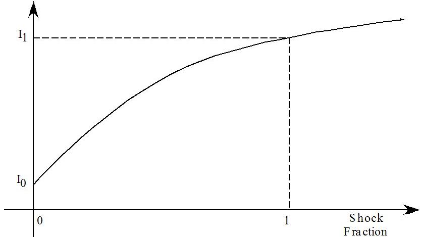
Figure 51.2 shows the effect of an import volume quota whose value is less than I1 . Then imports increase until they reach the quota and then level out.
Figure 51.2 Import quota
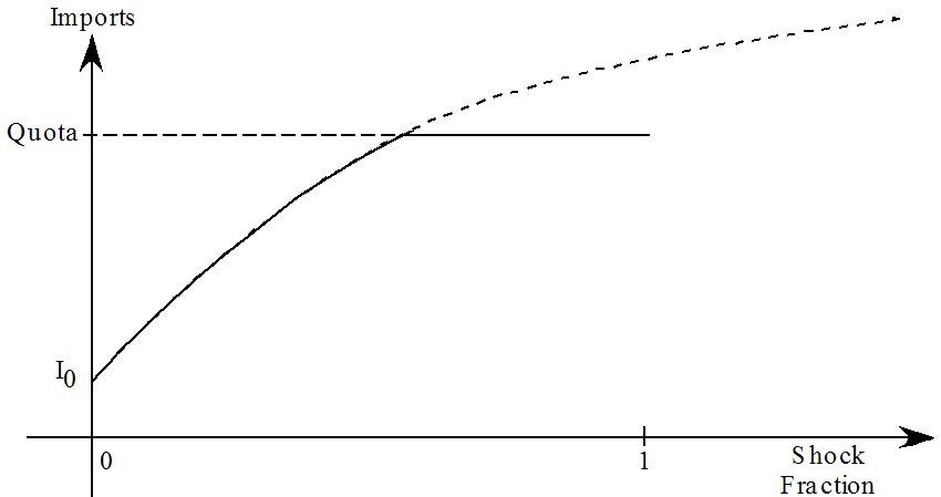
Figure 51.3 shows the import volumes (with an import quota in place) after each step of a 7-step Euler without a Newton correction term. During step number 4, the import volume jumps above the quota. During the remaining steps, its value stays at the same level (above the quota).
Figure 51.3 Quota - Euler with no Newton correction
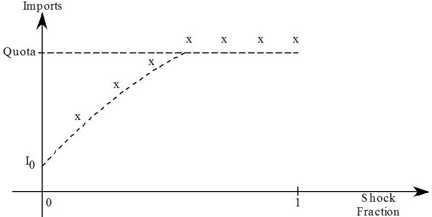
Figure 51.4 shows the difference that the Newton correction term makes: now imports go back to the quota during step 5 and remain on the quota for the rest of the simulation.
Figure 51.4 Quota - Euler with Newton correction
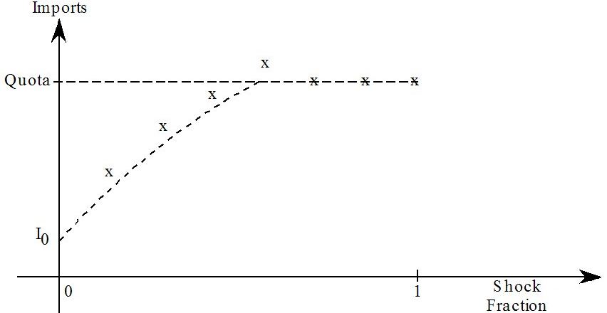
In general, these Newton corrections (bringing the import volume back to the quota volume if it goes above, or bringing the complementarity variable back above its lower bound of 1 if it should go below) ensure that the many-step Euler calculation has a very good chance of correctly finding the post-simulation states.
51.1.3 Combining the two ideas [gpd3.16.1.3]
The idea is to first carry out an Euler calculation (as in section 51.1.2) to try to find the post-simulation states. Then modify the original simulation as in section 51.1.1 to carry out an accurate simulation to obtain accurate results using extrapolation.
With the implementation described here, these two steps are automated. You start the simulation as usual by using a Command file. The following two steps are done within the same simulation.
- The software first carries out the Euler calculation. We call this the approximate run.
- Then, without any intervention by you, the software automatically modifies the closure and shocks to carry out the accurate run. The simulation results are those from the accurate run.
The software carries out checks to ensure that the post-simulation states (as estimated at the end of the approximate run) are those at the end of the accurate run. If not an error message is given. If you use automatic accuracy, the software automatically repeats the subinterval if such a problem occurs during any subinterval.
The rest of this chapter is an elaboration of these ideas.
51.2 States of the complementarity [gpd3.16.2]
Consider a general complementarity (see section 10.17)
L <=X<=U ⊥ EXP
which is notation for:
| Either | X = L | and | EXP > 0 |
| or | L<=X<=U | and | EXP = 0 |
| or | X=U | and | EXP < 0 |
See Figure 51.5 for this general complementarity.
Figure 51.5 General complementarity
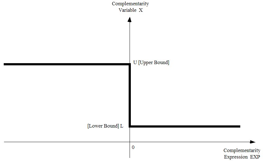
This means that there are three states associated with the general complementarity (see Figure 51.6).
State 1 (Variable Equal to Lower Bound)
The complementarity variable is equal to (or nearly equal to) its lower bound. [The complementarity expression should be positive or zero in this state.]
| X=L | and | EXP>0 |
State 2 (Expression Equal to Zero)
The complementarity expression is zero (or very nearly zero). [The complementarity variable should be in the range bounded by the lower and upper bounds.]
| L<=X<=U | and | EXP=0 |
State 3 (Variable Equal to Upper Bound)
The complementarity variable is equal to (or nearly equal to) its upper bound. [The complementarity expression should be negative or zero in this state.]
| X=U | and | EXP<0 |
As usual with GEMPACK, your pre-simulation data must be a solution of the model. This means that each component of the complementarity variable and the associated complementarity expression must be clearly in one of the above states in the pre-simulation data.
Figure 51.6 Three states of the general complementarity
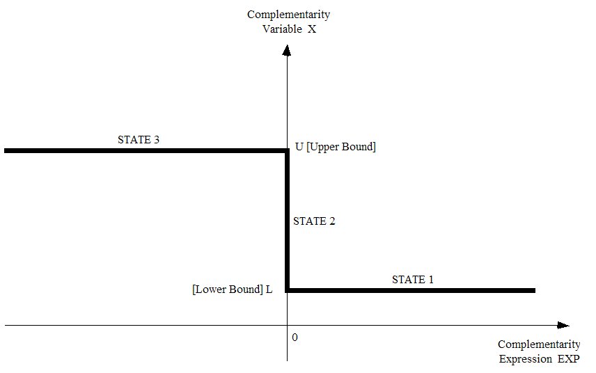
51.2.1 Complementarities with only one bound [gpd3.16.2.1]
First consider a Complementarity with only a lower bound
COMPLEMENTARITY (VARIABLE = X, LOWER_BOUND = L) comp1 Expression ;
This means that:
| Either | X = L | and | Expression > 0 | [State 1 - Variable Equal to Lower Bound] |
| or | X >= L | and | Expression = 0 | [State 2 - Expression Equal to Zero]. |
[Note that, when there is only a lower bound, there is no state 3, just states 1 and 2.]
Secondly consider a Complementarity with only an upper bound
COMPLEMENTARITY (VARIABLE = X, UPPER_BOUND = U) comp1 Expression ;
This means that:
| Either | X <= U | and | Expression = 0 | [State 2 - Expression Equal to Zero] |
| or | X = U | and | Expression < 0 | [State 3 - Variable Equal to Upper Bound]. |
[Note that, when there is only an upper bound, there is no state 1, just states 2 and 3.]
51.3 Writing the TABLO code for complementarities [gpd3.16.3]
The first step in using complementarities to model import, export or tariff rate quotas or other inequality constraints is to write in your TABLO Input file the additional TABLO code expressing the complementarity. The syntax for Complementarity statements is specified in section 10.17 and finer details of the semantics are in section 11.14. In the following section 51.3.1, there is a simple and fairly complete example of import quotas expressed as a complementarity. In section 51.3.2 this complementarity is added to a simple existing model (Miniature ORANI).
51.3.1 Import quota example [gpd3.16.3.1]
Volume quotas are applied to imports of commodities, which causes an extra import tariff, due to the quota, to be added to the existing import tariff.
XIMP_QUOTA(i) is the volume import quota and XIMP(i) is the volume of imports.
TIMP_QUOTA(i) is the extra power of the import tariff due to the import volume quota.
To write this complementarity, the variable XIMP_RATIO(i) is introduced, where
XIMP_RATIO(i) = XIMP(i)/XIMP_QUOTA(i)
is the ratio between the current volume of imports XIMP(i) and the quota volume XIMP_QUOTA(i). It is easy to see when the quota has been reached since then XIMP_RATIO is 1.0.
The complementarity expression can be written as 1-XIMP_RATIO(i).
The TABLO notation for the complementarity is :
COMPLEMENTARITY (Variable = TIMP_QUOTA, Lower_Bound = 1) IMPQUOTA (all,i,COM) 1.0 - XIMP_RATIO(i) ;
If the quota is not binding, XIMP(i) < XIMP_QUOTA(i) so that
XIMP_RATIO(i) < 1.0 that is, 1.0 - XIMP_RATIO(i) > 0
or, if the quota is binding, XIMP(i) = XIMP_QUOTA(i) so that
XIMP_RATIO(i) = 1.0 that is, 1.0 - XIMP_RATIO(i) = 0 .
In the pre-simulation data, the values TIMP_QUOTA(i) and XIMP_RATIO(i) must be in either State 1 or State 2 where the states are defined as:
| State 1 | (Quota not binding) | TIMP_QUOTA(i) = 1 | and | 1.0 - XIMP_RATIO(i) > 0 |
| State 2 | (Quota binding) | TIMP_QUOTA(i) >= 1 | and | 1.0 - XIMP_RATIO(i) = 0 |
It would be wrong to have TIMP_QUOTA(i) = 1 and XIMP_RATIO(i) > 1.0 for any commodity i in the pre-simulation data. (In economic terms this would mean imports XIMP were above quota in the pre-simulation data.)
51.3.2 Example: MOIQ (miniature ORANI with import quotas) [gpd3.16.3.2]
A simple example of import quotas is adding import quotas to the standard Miniature ORANI model MO.TAB.
The various files referred to here can be found in the file MOQ.ZIP which should be in the EXAMPLES subdirectory supplied with the GEMPACK software.
The files needed are
- MOIQ.TAB the TABLO Input file,
- MO.DAT the usual MO data file,
- MOIQ_RAT.DAT, the supplementary GEMPACK text data file containing import quota data,
- MOIQ1C.CMF, MOIQ1D.CMF and MOIQ1CX.CMF - Command files for this model.
MOIQ.TAB is the TABLO Input file for Miniature ORANI with import quotas added.
The supplementary data is in the text file MOIQ_RAT.DAT. In this data, imports of both commodities are in-quota. Imports of commodity 1 are 0.8 of the quota while imports of commodity 2 are 0.9 of the quota. The Complementarity statement is the same as in the previous section 51.3.1.
Various simulations with MOIQ are used in section 51.4 below to give you hands-on experience with simulations involving Complementarities. If you are keen to carry out a simulation with MOIQ now, go through the steps in section 51.4.1 below, and then return here to read the rest of this section (51.3).
Below we show you the Complementarity-related parts of MOIQ.TAB.
TABLO code from MOIQ.TAB
SET COM # commodities # (c1,c2) ; SET SOURCE # source of commodities # ( domestic, imported ) ; VARIABLE(DEFAULT=LEVELS) ; VARIABLE (all,i,COM)(all,s,SOURCE) PCOM(i,s) # commodity prices # ; (all,i,COM) PIMP(i) # import prices (foreign dollars) # ; (all,i,COM) XIMP(i) # import quantities # ; ! Change T(i) to TIMP(i) (WAS) T(i) # power of import duty #! (all,i,COM) TIMP(i) # power of import duty # ; PHI # exchange rate # ; ! etc .....[All statements above here are in the standard MO.TAB.] ! ! ADDITION FOR IMPORT VOLUME QUOTAS ! ! Set defaults for Levels variables and equations ! EQUATION(DEFAULT=LEVELS) ; VARIABLE(DEFAULT=LEVELS) ; FORMULA(DEFAULT=INITIAL) ; COEFFICIENT(DEFAULT=PARAMETER) ; Variable (GT 0) (All,i,COM) XIMP_QUOTA(i) # import volume quotas # ; Variable (All,i,COM) XIMP_RATIO(i) # ratios of import volume to import volume quota # ; Variable (All,i,COM) TIMP_QUOTA(i) # EXTRA power of import tariff due to import quota # ; FILE (TEXT) quota_ratios # Text file containing quota ratios # ; READ TIMP_QUOTA FROM FILE quota_ratios ; READ XIMP_RATIO FROM FILE quota_ratios ; Formula (Initial)(All,i,COM) XIMP_QUOTA(i) = XIMP(i)/XIMP_RATIO(i) ; Equation E_XIMP_RATIO ! (All,i,COM) XIMP_RATIO(i) = XIMP(i)/XIMP_QUOTA(i) ;! (All,i,COM) XIMP_RATIO(i)*XIMP_QUOTA(i) = XIMP(i) ; ! Original version of ZPPROFIMP equation must be modified to add TIMP_QUOTA ! FORMULA & EQUATION ZPPROFIMP ! Zero pure profits in importing commodity i - DPSV (5.36) ! !(ORIG) (all,i,COM) TIMP(i) = PCOM(i,"imported") / (PHI * PIMP(i));! (all,i,COM) TIMP(i) = PCOM(i,"imported") / (PHI * PIMP(i) * TIMP_QUOTA(i)) ; COMPLEMENTARITY (Variable = TIMP_QUOTA, Lower_Bound = 1) IMPQUOTA (All,i,COM) 1 - XIMP_RATIO(i) ;
51.3.3 Specifying bounds for the complementarity variable [gpd3.16.3.3]
When you write down the COMPLEMENTARITY statement, you specify the bounds for the complementarity variable via the LOWER_BOUND and UPPER_BOUND qualifiers. We recommend that you do not also specify these bounds via GE,LE qualifiers (see, for example, section 25.4) when you declare the complementarity variable.
For example, in the Import Quota Example just above, when you declare the complementarity variable TIMP_QUOTA do not include "(GE 1)". Rather declare it via
Variable (Levels) (All,i,COM) TIMP_QUOTA(i) ;
The Complementarity statement ensures that TIMP_QUOTA(i) >= 1.
51.3.4 Scale the complementarity expression if possible [gpd3.16.3.4]
It may be desirable to write down the complementarity expression in a way which makes it well scaled in the sense that its (levels) values are about the same size as those of the complementarity variable. A tariff example will make this clear.
Consider MOIQ.TAB (see sections 51.3.1 and 51.3.2 above). The complementarity variable is TIMP_QUOTA(i), the extra power of the import tariff due to the import quota. It has lower bound 1. The complementarity expression we use in MOIQ.TAB is
| 1 - XIMP_RATIO(i) | [1] |
where XIMP_RATIO(i) is equal to XIMP(i)/XIMP_QUOTA(i) which is the ratio between the current import volume XIMP(i) and the quota volume XIMP_QUOTA(i). So the values of this complementarity expression are somewhere between zero and 1. Thus the values of this expression and of the complementarity variable TIMP_QUOTA are roughly of the same magnitude.
Contrast the above form of the complementarity expression with perhaps the more natural
| XIMP_QUOTA(i) - XIMP(i) | [2] |
This has the same property as the expression [1] above, namely that it is either positive or zero and is zero when the complementarity variable is greater than the lower bound of 1. But the units of XIMP_QUOTA and XIMP may be quite different from those of TIMP_QUOTA. For example, the natural values to use for XIMP(i) are the values of imports as held on the pre-simulation data base. If these are held in dollars, they may be very large (perhaps in millions or larger).
The two complementarity expressions [1] and [2] above are equally good theoretically. But they may have different numerical properties. When carrying out complementarity simulations, the software needs to add or subtract the values of the complementarity variable and expression in order to estimate which state each component is. This addition or subtraction is more reliable numerically if the numbers being added or subtracted are about the same size. This is why we suggest that you try to scale the complementarity expression.3
If Possible Scale Bounds and Expression to be About 1
The programs endeavour to find out if the relevant states are fairly exact at the end of the accurate run (see section 51.7.5). Their reports will be more sensible if you are able to scale both the Complementarity Expression and Variable Bounds to of the same order of magnitude as 1. [For example, values between 0 and 5 for the bounds and expression would be ideal.]
We realise that this may not always be possible.
51.3.5 Levels variables are required [gpd3.16.3.5]
COMPLEMENTARITY statements require levels variables, both for the Complementarity Variable and in the Complementarity Expression.
This may appear to cause a problem when the rest of the TABLO Input file contains only linear variables and equations. However it turns out to be relatively easy to write TABLO code linking the levels variables needed for the COMPLEMENTARITY statement to the linear variables in the rest of the TABLO Input file. Below we discuss this issue in detail in two of the example models (see sections 51.8.4 and 51.8.7 below).
You will need to gain experience in writing this "linking" code if you wish to add a Complementarity to an existing linearized model. We suggest that you start by looking closely at the two examples referred to in the previous paragraph. Note also that the LINEAR_VAR= and LINEAR_NAME= Variable qualifiers (see section 9.2.2) are useful in this context.
51.3.6 Complementarities are related to MAX and MIN [gpd3.16.3.6]
Complementarities with a single bound (lower or upper) can be expressed in terms of MIN (minimum) and/or MAX (maximum), as we indicate below.
First consider a Complementarity with only a lower bound.
COMPLEMENTARITY (VARIABLE = X, LOWER_BOUND = L) comp1 EXP1 ;
This means that:
Either X = L and EXP1 > 0, or X >= L and EXP1 = 0.
Equivalently,
Either X - L = 0 and EXP1 > 0, or X - L >= 0 and EXP1 = 0,
which is the same as:
MIN( X - L, EXP1 ) = 0.
Secondly consider a Complementarity with only an upper bound.
COMPLEMENTARITY (VARIABLE = X, UPPER_BOUND = U) comp1 EXP1 ;
This means that:
Either X <= U and EXP1 = 0, or X = U and EXP1 < 0.
Equivalently,
Either X - U <= 0 and EXP1 = 0, or X - U = 0 and EXP1 < 0,
which is the same as:
MAX( X - U, EXP1 ) = 0.
Finally note that MAX(A,B)=0 is equivalent to MIN(-A,-B)=0, so that any complementarity with a single bound can be expressed in terms of either MAX or MIN.
51.3.7 Equivalent ways of expressing complementarities with a single bound [gpd3.16.3.7]
Consider the import quota example from above.
COMPLEMENTARITY (Variable = TIMP_QUOTA, Lower_Bound = 1) ImpQuota (all,i,COM) 1.0 - XIMP_RATIO(i) ;
or
COMPLEMENTARITY (Variable = TIMP_QUOTA, Lower_Bound = 1) ImpQuota2 (all,i,COM) XIMP_QUOTA(i) - XIMP(i) ;
It is easy to see that this can be written equivalently as
COMPLEMENTARITY (Variable = XIMP, Upper_Bound = XIMP_QUOTA) ImpQuota3 (all,i,COM) 1 - TIMP_QUOTA(i) ;
since this means that
| Either | XIMP(i) < XIMP_QUOTA(i) | and | 1 - TIMP_QUOTA(i) = 0 | [quota not binding], |
| or | XIMP(i) = XIMP_QUOTA(i) | and | 1 - TIMP_QUOTA(i) < 0 | [quota is binding]. |
More generally, any Complementarity with a single bound can be rewritten with what is the complementarity variable in the original complementarity becoming part of the complementarity expression in the rewritten complementarity, as we explain below.
Complementarity with only a lower bound.
COMPLEMENTARITY (VARIABLE = X, LOWER_BOUND = L) comp1 EXP1 ;
This means that:
Either X = L and EXP1 > 0, or X >= L and EXP1 = 0.
Introduce a new (levels) variable V and an equation saying that
V = EXP1.
Then V >= 0 (since EXP1 is >= 0). Hence the original complementarity can written as
COMPLEMENTARITY (VARIABLE = V, LOWER_BOUND = 0) comp1a X - L ;
since this means that
Either V = 0 and X - L > 0, or V >= 0 and X - L = 0.
In this alternative way of writing the complementarity, what was the complementarity variable in the original form has become part of the complementarity expression. The original complementarity has been rewritten as a different complementarity statement plus a new equation (the one linking V and EXP1).
Import Quota Example
Consider again the import quota example from above.
COMPLEMENTARITY (Variable = TIMP_QUOTA, Lower_Bound = 1) ImpQuota (all,i,COM) XIMP_QUOTA(i) - XIMP(i) ;
Following the ideas above this could be rewritten as the equation
(All,i,COM) V(i) = XIMP_QUOTA(i)- XIMP(i)
and the complementarity
COMPLEMENTARITY (Variable = V, Lower_Bound = 0) ImpQuota4 (all,i,COM) TIMP_QUOTA(i) - 1 ;
Complementarity with only an upper bound.
COMPLEMENTARITY (VARIABLE = X, UPPER_BOUND = U) comp2 EXP1 ;
This means that:
| Either | X <= U | and | EXP1 = 0, |
| or | X = U | and | EXP1 < 0. |
Introduce a new (levels) variable W and an equation saying that
W = EXP1.
Then W <= 0 (since EXP1 is <= 0). Hence the original complementarity can written as
COMPLEMENTARITY (VARIABLE = W, UPPER_BOUND = 0) comp2a U - X ;
since this means that
| Either | W <= 0 | and | U - X = 0, |
| or | W = 0 | and | U - X < 0. |
51.4 Hands-on examples with MOIQ [gpd3.16.4]
In this section we introduce you to hands-on simulations, taking MOIQ (Miniature ORANI with Import Quotas — see section 51.3.2 above) as the example model. We recommend that you run these complementarity simulations now, and check the outputs and LOG file, since then you will be in a better position to follow the discussion about complementarities in the rest of this chapter.
The various files referred to here can be found in the file MOQ.ZIP which should be in the EXAMPLES subdirectory supplied with the GEMPACK software. The files needed are
- MOIQ.TAB the TABLO Input file (see section 51.3.2),
- MO.DAT the usual MO data file,
- MOIQ_RAT.DAT, the supplementary text data file containing import quota data (see section 51.3.2),
- MOIQ1C.CMF, MOIQ1D.CMF and MOIQ1CX.CMF - Command files for this model.
To prepare for these simulations, run TABLO on MOIQ.TAB in the usual way, either producing the TABLO-generated program executable image MOIQ.EXE or the GEMSIM Auxiliary files MOIQ.GSS and MOIQ.GST.
51.4.1 Decreasing a quota volume - command file MOIQ1C.CMF [gpd3.16.4.1]
In the simulation in Command file MOIQ1C.CMF, the quota volume for commodity 1 is decreased by 30%. Since imports of commodity 1 are originally 0.8 of the quota, you would expect this to make the quota binding for commodity 1.
Run the simulation from the Command file4.
You will see indeed that imports of commodity 1 end up on-quota. The post-sim value of TIMP_QUOTA("c1") is 1.237 (which is larger than its lower bound of 1).
Look at the results using AnalyseGE. In AnalyseGE., open the Solution file MOIQ1C.SL4. Search for the COMPLEMENTARITY statement in the TAB file (in the TABmate window of AnalyseGE) and right-click on it. Select Show State and Variable Values.
| STATE-PRE | STATE-POST | VAR-PRE | VAR-POST | EXP-PRE | EXP-POST | LB-PRE | LB-POST | |
| c1 | 1 | 2 | 1 | 1.2374 | 0.2 | 0 | 1 | 1 |
| c2 | 1 | 1 | 1 | 1 | 0.1 | 0.049 | 1 | 1 |
The table5 shows that the pre-sim value of the complementarity variable (VAR-PRE) for commodity 1 is 1.0 and pre-sim value of the complementarity expression (EXP-PRE) for commodity 1 is 0.2. Both values are consistent with commodity 1 being in-quota.
The table shows that the post-sim value for commodity 1 of the complementarity variable (VAR-POST) is 1.2374 and expression (EXP-POST) is 0.0. Both values are consistent with the quota for commodity 1 being binding after the simulation.
The table also shows that the value of the complementarity expression for commodity 2 has decreased from the pre-simulation value (EXP-PRE) of 0.1 to a post-simulation value (EXP-POST) of 0.0490. Thus imports of commodity 2 increase in volume but remain in-quota.
The first two columns show that commodity 1 pre-simulation (STATE-PRE) is in State 1 (Complementarity variable equal to lower bound) and post-simulation (STATE-POST) is in State 2 (Expression equal to zero).
It is also instructive to look at the updated supplementary data in file MOIQ1CQ.UPD. This shows the post-sim values for the complementarity variables TIMP_QUOTA and for XIMP_RATIO.
Look at the Command file MOIQ1C.CMF used in this run. Most of the statements are ones you are familiar with. In fact the only unusual statement is
Complementarity steps_approx_run = 20 ;
This tells the program how many Euler steps to use in the approximate run (see section 51.6 below).
Now look at the LOG file MOIQ1C.LOG produced from this run6. You will see that
(A) The program first carries out the approximate run. There are 20 Euler steps.
(B) At the end of the first step of the approximate run, the program reports the initial states for the complementarity IMPQUOTA. The report says.
[Complementarity IMPQUOTA. Numbers initially in states 1 and 2 are 2 and 0 respectively.]
(C) During step 14 of the approximate run, the program reports a state change for commodity "c1". The report is:
[Complementarity IMPQUOTA("c1"):
State change from 1 to 2 during this step.
Occurs after 0.52873969 part of the step.]
This means that the quota for commodity "c1" has gone from non-binding (state 1 — see section 51.2 above) to binding (state 2).
(D) After the approximate run, the program says that it is beginning the accurate run. It also reports the states and changes found over the approximate run. This part of the LOG file is:
===> Beginning accurate complementarity calculation.
[Processing complementarity IMPQUOTA.]
[Are 1 changing from state 1 to state 2, and
0 changing from state 2 to state 1.]
[Are 1 remaining unchanged in state 1, and
0 remaining unchanged in state 2.]
[Total numbers in post-sim states 1 and 2 are
1 and 1 respectively.]
(E) Then the accurate run begins. This is a Gragg 6,8,10-step calculation, as requested in the Command file.
(F) At the end of the accurate run, the program checks to see if the states are the same as they were at the end of the approximate run. [If they were not, the program would report an error.] Since they are, the program reports the states:
Summary of state changes over whole simulation:
[Processing complementarity IMPQUOTA.]
[Are 1 changing from state 1 to state 2, and
0 changing from state 2 to state 1.]
[Are 1 remaining unchanged in state 1, and
0 remaining unchanged in state 2.]
[Total numbers in post-sim states 1 and 2 are. 1 and 1 respectively.]
and then indicates that the simulation has ended without error.
(G) In fact the program changed the closure for the accurate run to make imports of commodity "c1" exogenous (set to the level of the quota). This is done since the approximate run indicated that the quota would become binding for "c1". Notice that you did not need to intervene to achieve this. Nor is there anything in the Command file to suggest how the program should change the closure on the accurate run — this is deduced from the Complementarity statement in the TABLO Input file.
51.4.2 Decreasing both quota volumes - command file MOIQ1D.CMF [gpd3.16.4.2]
In this simulation, the quota volume for commodity 1 is decreased by 30% as for MOIQ1C above. Also the quota volume for commodity 2 is decreased by 25% which makes it also binding.
You might like to run this and check the points referred to above for the MOIQ1C simulation. In particular,
- check the post-simulation states and the post-simulation values of the Complementarity variables and expressions via AnalyseGE.
- check from the log file MOIQ1D.LOG when the states change during the approximate run.
51.4.3 No approximate run - command file MOIQ1CX.CMF [gpd3.16.4.3]
This is the MOIQ1C simulation (see section 51.4.1 above) except that the statement
complementarity do_approx_run = no ;
(see section 51.6 below) is added to the Command file. This instructs the program not to carry out the approximate run first. The state change which should occur with these shocks (the quota on commodity c1 should become binding) does not happen. Instead the post-simulation values of the complementarity variable TIMP_QUOTA end up being considerably lower than the specified lower bound of 1 for each commodity. The simulation ends with an error. The program reports that the simulation should be rerun, doing the approximate run first, in order to get the correct results.
We suggest that you run this simulation and look at the log file (start at the end) to confirm the points in the paragraph above.
51.5 Other features of complementarity simulations [gpd3.16.5]
In this section we comment on some other features of Complementarity simulations.
51.5.1 Closure and shocks [gpd3.16.5.1]
All components of the complementarity variable which are relevant to the complementarity must be endogenous. This must be a consequence of the closure in the Command file for the simulation.
For example, in the Import Quota example in section 51.3.1 above, all components of the variable TIMP_QUOTA must be endogenous.
If the complementarity only applies to subsets of the sets that the complementarity variable is defined over, the complementarity variable must be endogenous over the correct subsets. For example, consider
Variable(levels) (All,i,S1),(all,j,S2) V(i,j) ;
Variable(levels) (All,i,LS1),(all,j,LS2) L(i,j) ;
Coefficient(parameter) (All,i,US1),(all,j,US2) U(i,j) ;
Complementarity (Variable = V,
Lower_bound = L, Upper_bound=U) Comp1
(all, i, T1)(all, j, T2) X(i,j) - Y(i,j) ;
In this case the complementarity variable V(i,j) must be endogenous for all i in the set T1 and all j in the set T2. [Note that T1 must be equal to or a subset of each of S1, LS1 and US1 (see section 11.14). Similarly, T2 must be equal to or a subset of each of S2, LS2 and US2.]
When TABLO comes across a COMPLEMENTARITY statement, it automatically adds some levels variables (see section 51.7.2 below). When you specify the closure and shocks, you should not list the extra variables automatically added by TABLO in your closure as either endogenous or exogenous. The simulation program (GEMSIM or the TABLO-generated program) automatically sets these variables to be exogenous or endogenous as required, and gives a shock of 1 to the variable $del_comp.
In the example at the end of section 11.14, all components of $comp1@D and $del_Comp are exogenous and all components of c_comp1@E are endogenous. However these variables should not appear in the closure in specified in the Command file you use to run the simulation.
More details about these extra variables are given in section 51.7.2 below.
In counting up the number of equations to balance with the number of endogenous variables, the complementarity is equivalent to an equation with the same quantifier list.
For example, in the import volume quota example MOIQ.TAB in section 51.3.2,
- three new (levels) variables, XIMP_QUOTA, XIMP_RATIO and TIMP_QUOTA were added.
- one new equation E_XIMP_RATIO was added, and
- one COMPLEMENTARITY was added.
[These are the additions made to the standard MO.TAB file.]
This is like adding 3 COM variables and 2 COM equations. Thus it is necessary to specify one extra COM variable as exogenous when running a simulation.
In the Command file MOIQ1C.CMF (see section 51.4.1), the variable XIMP_QUOTA was added to the exogenous list.
51.5.2 Running TABLO and simulations [gpd3.16.5.2]
After writing the TABLO code for the model containing a complementarity, use TABLO to implement the model in the normal way. You can carry out condensation if your model is usually condensed - details of restrictions on condensation are in section 11.14.1.
To run the simulation, just use a Command file in the usual way. The program first does an approximate version of the simulation. Then an accurate version is run, all as part of the same simulation. You do not need to specify anything about the approximate run, or carry out any separate steps to make the approximate run occur.
51.5.3 Program reports state changes [gpd3.16.5.3]
While carrying out the multi-step Euler approximate simulation, the program reports
- the initial states of the complementarities before the simulation,
- state changes as they occur during the calculation,
- a summary of the state changes that have occurred over the whole approximate run.
You have already seen these reports for the MOIQ1C simulation in section 51.4.1 above.
51.5.4 Program checks states and bounds at end of run [gpd3.16.5.4]
After the accurate run, the program checks
- that the post-simulation states are the same as those found after the approximate run, and
- that the post-simulation values of the complementarity variables are within the specified bounds.
If either of these fails, a fatal error is generated [unless you are doing automatic accuracy, in which case the subinterval is redone, or unless you have the statement "complementarity state/bound_error = warn ;" (see section 51.6) in your Command file].
51.5.5 Checking the simulation results [gpd3.16.5.5]
As with any simulation, you must check that the simulation has accurate results, that is that the simulation has converged satisfactorily. Look either at the Extrapolation Accuracy Summaries (see section 26.2) on the Log file or, in detail, at the Extrapolation file (.XAC). [In checking these results, you can ignore non-convergence of the dummy variables added by TABLO (see section 51.7.2 below), since these play no role in the accurate simulation.]
As usual, if the simulation is highly non-linear, it may need more steps (or automatic accuracy) in order to produce sufficiently accurate results. If you think this is why the accurate simulation has not produced good results, increase the number of steps in your Command file, or ask for automatic accuracy. [See section 26.1 for general suggestions. See also section 51.7.4.]
51.5.6 Omitting the accurate run [gpd3.16.5.6]
It is possible to do just the approximate run and then stop if you include the statement
complementarity do_acc_run = no ;
in your Command file. For example, if your model is very large and takes a long time to solve, you may be reluctant to double the total solve time and may be content with the results of the approximate run. Note that, if a Complementarity changes state, because of the way that steps are redone with a Newton correction (see, for example, 51.4 above), the approximate run will produce more accurate results than would be produced by a single Euler solution which ignores the complementarity.
There are several restrictions in this case.
- The solution method must be Euler.
- You must ask for a single multi-step Euler solution (any number of steps).
- You must specify only one subinterval.
- You must not specify automatic accuracy.
51.5.7 Subtotals when there are complementarities [gpd3.16.5.6a]
It turns out that subtotals in models with complementarities need careful handling. We describe in chapter 52 how you should calculate subtotals in models containing complementarities. However, do not attempt to read that chapter until you are familiar with the material in this chapter.
51.6 Command file statements for complementarity simulations [gpd3.16.6]
To specify the number of Euler steps in the approximate run
The following statement is optional. You only need to add it if the default is not satisfactory. If the following statement is not present the default is the sum of the numbers of steps used in the accurate simulation. For example, if, in the Command file, you ask for Gragg with steps (8, 10, 12), then the default is to use 30 (=8+10+12) Euler steps in the approximate simulation.
complementarity steps_approx_run = ddd ;
where ddd is the number of Euler steps to use.
For example, if you want 10 Euler steps in the approximate run, include the statement
complementarity steps_approx_run = 10 ;
The actual number of steps may be more than you specify. This is because a step may be redone (see section 51.7.3).
Omit the Approximate Run
If you think that the shocks will not change any states, you can save time by not doing the approximate run. In this case, you can add the statement
complementarity do_approx_run = no ; ! default is YES
to your Command file. The software checks to see if the pre-simulation and post-simulation states are the same, and also to see if the complementarity variables are within the bounds specified in the complementarity statements. If the pre-sim and post-sim states are not the same, or if any complementarity variable is outside the bounds specified, the program reports this and sets a fatal error. Even if there is an error, all files (including the Solution, updated data and SLC files) are kept. Whether there is an error or not, the complementarity arrays are added to the SLC file so that you can look at them in AnalyseGE.
You must be very careful to check that the results obtained are sufficiently accurate (that is, have converged). [They may not converge if in fact, one or more state changes should occur as a consequence of the shocks.]
An example is the Command file MOIQ1CX.CMF supplied with MOIQ.TAB (see section 51.4.3 above). With the shocks in this Command file, the complementarity IMPQUOTA("c1") should change from state 1 (in-quota) to state 2 (quota is binding). But, because of the statement "complementarity do_approx_run = no ;" in MOIQ1CX.CMF, this state change is not picked up. Instead the post-simulation values of the complementarity variables TIMP_QUOTA("c1") and TIMP_QUOTA("c2") are reported to be significantly less than the specified lower bound of 1. This is what indicates that a state change should occur. The run ends with a message saying that the simulation has failed and suggesting that you remove the statement "complementarity do_approx_run = no ;" and then rerun the simulation.
Do Not Redo a Step if State Changes During Approximate Run
Normally, if one or more states change during a step in the approximate run, the step is redone with a shorter step length so that the state change occurs just before the end of the step (see section 51.7.3). While redoing steps can slow down the approximate run, the extra accuracy achieved is usually worth the extra time. If you do not want steps to be redone in this way, you can include the statement (which we do not recommend)
complementarity redo_steps = no ; ! default is YES
in your Command file.
Step Length when Redo Step
Normally, if one or more states change during a step in the approximate run, the step is redone with a shorter step length so that the state change occurs just before the end of the step (see section 51.7.3). If a state change occurs very early in the step, the step length of the redone step may be very small. You can control the minimum step length for redone steps by putting a statement of the form
complementarity redo_step_min_fraction = <number> ; ! default is 0.005
For example, if you put the <number> equal to 0.01, the step length of the redone step will never be less then 0.01 times the length of the original step7. If you do not include such a statement, the program will use the default value of 0.005.
Treat State or Bound Errors as Warnings Only
Normally state or bound errors discovered after the end of the accurate run (see section 51.5.4) are regarded as fatal errors (unless you are using automatic accuracy, in which case the subinterval is redone). If you wish these errors to be treated only as warnings, you can include the statement
complementarity state/bound_error = warn ; ! default is FATAL
in your Command file. If you include this statement (which we do not recommend), it is your responsibility to check your log file carefully for the relevant warnings.
Omit the Accurate Run
Normally the approximate run is followed by the accurate run. If you wish to just carry out the approximate run and then stop, you can include the statement
complementarity do_acc_run = no ; ! default is YES
in your Command file. See section 51.5.6 for more details about this option. In particular, there are some restrictions on when this is allowed.
51.7 Technical details about complementarity simulations [gpd3.16.7]
In this section we give technical details about complementarity simulations. You can probably ignore most of these on a first reading.
51.7.1 How the closure and shocks change for the accurate simulation [gpd3.16.7.1]
After running the approximate simulation, the program has estimates of the post-simulation states for each component relevant to each complementarity.
For each component of each complementarity, the program changes closure and gives extra shocks as described below.
1. Suppose that the post-sim state is state 2.
Then the post-sim value of the complementarity expression is zero. This component of the complementarity expression is made exogenous and shocked to the value zero. Since the program can calculate the pre-simulation levels value of this expression, it can calculate the shock.
2. Suppose that the post-sim state is 1.
Then the post-sim value of the complementarity variable must equal the post-sim value of the lower bound.
(a) Suppose that the lower bound is a constant, a parameter or a levels variable for which this component is exogenous. Then the post-sim levels value of the complementarity variable is known (exactly). Accordingly this component of the complementarity variable is made exogenous and shocked to the desired value. Since the program can calculate the pre-simulation levels value of this variable, it can calculate the shock.
(b) Suppose that the lower bound is a levels variable for which this component is endogenous. Then we cannot be sure of the exact post-sim levels value of this lower bound. Accordingly it is not a good idea to proceed as in (a). Instead the variable which is the difference between the complementarity variable and the lower bound is used. [Whenever the lower bound is a levels variable, this variable is introduced automatically by TABLO — see section 51.7.2 below.] The post-sim value of this variable must be zero. This component of this variable is made exogenous and shocked to zero. Since the program can calculate the pre-sim levels value of the complementarity variable and of the lower bound, it can calculate the pre-sim levels value of this variable (the difference between them). Hence the shock can be calculated exactly.
3. Suppose that the post-sim state is 3.
Then, we proceed as in 2. above (just replacing lower bound by upper bound). Either
(a) this component of the complementarity variable is made exogenous and shocked to the known post-sim upper bound, or
(b) this component of the variable equal to the difference between the complementarity variable and the upper bound variable is made exogenous and shocked to the post-sim value zero.
Hence, for every component of the complementarity, one component of one of the relevant variables is made exogenous. [This is either the complementarity expression when the post-sim state is 2, the complementarity variable or the variable which is the difference between this and the lower/upper bound when the post-sim state is 1 or 3.]
To keep the closure correct, ALL components of the complementarity dummy variable (see section 51.7.2 below) are made endogenous. This turns off the non-differentiable equation used as a translation of the complementarity during the approximate calculation.
Since these equations are the only non-differentiable equations in the system, the accurate simulation should converge using extrapolation.
When you carry out a simulation involving one or more complementarities via GEMPACK, the program (GEMSIM or a TABLO-generated program) sets up the new closure and extra shocks after the approximate run and uses this new closure and extra shocks for the accurate calculation.
Examples
Simulation in MOIQ1C.CMF
[This simulation was described in section 51.4.1 above.]
For commodity 1 the post-sim state is 2 (while the pre-sim state is 1). This means that commodity 1 of the complementarity expression is set exogenous in the accurate simulation. [The levels, change variable IMPQUOTA@E is introduced by TABLO and set equal to the complementarity expression via the equation E_IMPQUOTA@E — see section 51.7.2 where we describe the extra variables introduced.] Component 1 of this variable IMPQUOTA@E is shocked from its pre-sim value of 0.2 to the post-sim value of zero, so the shock is -0.2.
The post-sim state for commodity 2 is 1. Thus commodity 2 of the complementarity variable TIMP_QUOTA is made exogenous in the accurate simulation. This is shocked from its pre-simulation value of 1.0 (the lower bound) to its post-sim value, also 1.0. Thus the shock for this component is zero.
Simulation in MOTQ1C.CMF
[This simulation is described in section 51.8.2 below.]
For commodity 1 the post-sim state is 2 (while the pre-sim state is 1). This means that commodity 1 of the complementarity expression is set exogenous in the accurate simulation. [The levels, change variable TRQ@E is introduced by TABLO and set equal to the complementarity expression via the equation E_TRQ@E — see section 51.7.2 where we describe the extra variables introduced.] Component 1 of this variable TRQ@E is shocked from its pre-sim value of 0.25 to the post-sim value of zero, so the shock is -0.25.
The post-sim state for commodity 2 is 1. Thus commodity 2 of the complementarity variable TIMP_TRQ is made exogenous in the accurate simulation. This is shocked from its pre-simulation value of 1.0 (the lower bound) to its post-sim value, also 1.0. Thus the shock for this component is zero.
Simulation in MOTQ1D.CMF
[This simulation is described in section 51.8.2 below.]
For commodity 1 the post-sim state is 3 (while the pre-sim state is 1). Thus commodity 1 of the complementarity variable TIMP_TRQ is made exogenous in the accurate simulation. This is shocked from its pre-simulation value of 1.0 (the lower bound) to its post-sim value of 4.0 (the upper bound). Thus the shock for this component of TIMP_TRQ is 300% (since this is a percentage-change variable).
For commodity 2 the post-sim state is 2 (while the pre-sim state is 1). This means that commodity 2 of the complementarity expression is set exogenous in the accurate simulation. Component 2 of the associated variable TRQ@E is shocked from its pre-sim value of 0.20 to the post-sim value of zero, so the shock is -0.20.
51.7.2 Extra variables introduced with each complementarity [gpd3.16.7.2]
Extra variables are introduced for each complementarity as described below. However in general, these extra variables are of no concern to the user. The only restriction from the user's point of view is that all components of the complementarity variable must be endogenous.
(i) Complementarity expression. This levels, change variable is called
<comp-name>@E
The levels equation E_<comp-name>@E sets this variable equal to the complementarity expression.
(ii) Complementarity dummy variable. This linear, change variable is called
$<comp-name>@D
This variable appears in the complicated linear equation E_$<comp-name> (see, for example, the linear equation containing $del_Comp shown near the end of section 11.14) which captures the complementarity statement. This equation is used during the approximate run. This equation is turned off during the accurate simulation (by setting all components of the complementarity dummy variable to be endogenous).
(iii) Newton-correction variable $del_Comp. This is a scalar linear variable. Only one such variable is introduced even if there are several Complementarity statements in the TAB file. This same variable occurs in the linearized equations capturing each complementarity8. $del_Comp is a NO_SPLIT variable — the Variable qualifier "NO_SPLIT" is an alternative to "CHANGE" and "PERCENTAGE_CHANGE". It means that any shock given to this variable is given in full at each step of a multi-step calculation.
(iv) If there is a lower bound and if this lower bound is a levels variable, a levels, change variable is introduced. This is set equal to the difference between the complementarity variable and this lower bound variable. This levels variable is called
<comp-name>@L
The levels equation E_<comp-name>@L sets this variable equal to the complementarity variable minus the lower bound variable. [This variable will be needed in the accurate simulation if the post-sim state for some component is 1 and if this component of the lower bound variable is endogenous — see case 2(b) in section 51.7.1.]
(v) If there is an upper bound and if this upper bound is a levels variable, a levels, change variable is introduced. This is set equal to the difference between the complementarity variable and this upper bound variable. This levels variable is called
<comp-name>@U
The levels equation E_<comp-name>@U sets this variable equal to the complementarity variable minus the upper bound variable. [This variable will be needed in the accurate simulation if the post-sim state for some component is 1 and if this component of the lower bound variable is endogenous — see case 3(b) in section 51.7.1.]
During the approximate simulation9,
(a) all components of the complementarity variable must be endogenous (see section 51.5.1);
(b) the software automatically sets all components of the variable <comp-name>@E (set equal to the complementarity expression) endogenous;
(c) the software automatically sets all components of the complementarity dummy variable <comp-name>@D exogenous and not shocked;
(d) the software automatically sets the variable $del_Comp exogenous with a shock equal to 110 ;
(e) the software automatically sets all components of the complementarity variables <comp-name>@L and <comp-name>@U (if either exists) endogenous.
You must not mention any of the variables in (b)-(e) above in your Command file. The closure you set up in the Command file must satisfy (a). [If this does not seem possible, maybe you can express the complementarity in a slightly different way to accomplish this.]
However, variable $del_comp can be included in a subtotal statement (see section 29.1) in a Command file.
51.7.3 Step may be redone during approximate run [gpd3.16.7.3]
When a change of state occurs during one Euler step of the approximate run, this step is redone with a shorter step length so that the state change occurs just before the end of the step. This means that the simulation does not overshoot a bound by very much during the approximate run.
For example, in the MOIQ1C.CMF simulation (see section 51.4.1 above), the complementarity IMPQUOTA("c1") changes from state 1 (in-quota) to state 2 (on-quota) after about 0.529 of the 14th Euler step. This step is redone (reducing its length to a little over 52.9% of the original step length). When the step is redone, this complementarity IMPQUOTA("c1") changes state after approximately 0.995 of this new, shorter step. Thus the import volume of commodity "c1" only overshoots the quota by a very small amount on this rerun step11.
If two or more state changes occur during one Euler step of the approximate run, the step is redone with a shorter step length so that the state change which occurs first during the step occurs just before the end of the step. While this usually means that only one state change occurs during the redone step, it may happen that two or more occur since they occur at nearly the same stage during the step.
Because some steps may be redone, the actual number of steps in the approximate run may be more than you request in the "complementarity steps_approx_run = ... ;" statement (see section 51.6) in your Command file.
51.7.4 Several subintervals and automatic accuracy [gpd3.16.7.4]
As with any other simulation, you can request that the simulation be carried out over several subintervals (see section 26.3) or with automatic accuracy (see section 26.4).
If you specify several subintervals or automatic accuracy,
an approximate run is followed by an accurate run in each subinterval.
[You specify several subintervals by including a statement of the form "subintervals = ... ;" in your Command file (see section 26.3).
If you specify automatic accuracy, the software checks the accuracy at the end of each subinterval (as usual). It also checks that the complementarity part of the simulation has worked over this subinterval. For example, it checks that
- the post-simulation states after the accurate run for this subinterval are the same as the post-simulation states after the approximate run for this subinterval.
- the post-simulation values of the complementarity variables are within the required ranges.
If any of these tests fails, the subinterval is redone (with a shorter subinterval length). [An example is 1B5RAAX.CMF which is the same as 1B5RAA.CMF (see section 51.8.4 below) except that one subinterval is specified to start with. The attempt to do the whole simulation in one subinterval fails because the post-sim state for (sugar,AFR,USA) is 3 after the accurate simulation but 2 after the approximate simulation. The subinterval length is reduced and the simulation then proceeds ok.]
The advantage of specifying automatic accuracy with a relatively nonlinear simulation (for example, one with relatively large shocks) is that you do not need to experiment to determine how many Euler steps in a single subinterval are needed to satisfactorily predict the post-simulation states. An interesting example in this context is the 1B5R.CMF GTAP simulation (see section 51.8.4 below).
You specify automatic accuracy by including the statement "automatic accuracy = yes ;" in your Command file (see section 26.4). [You can also specify the length of the first subinterval via a statement of the form "subintervals = ... ;".]
If the approximate run is having difficulty finding the accurate post-simulation states (perhaps because of large shocks), we strongly recommend that you use several subintervals or automatic accuracy.
51.7.5 Checks that the pre- and post-simulation states are accurate [gpd3.16.7.5]
At the beginning of each simulation, the software checks that the data has each component of each complementarity accurately in one or other of the possible states. This means checking that the data represents points close to the exact graph of the complementarity. In terms of Figure 51.7, it means that all points lie within some dotted region close to the exact graph of the complementarity.
Similar checks are made at the end of the whole simulation (and at the end of each subinterval if there are several).
If any of the states is not exact (to within some tolerance represented by the dotted lines in Figure 51.7), a warning is issued. At present the software takes no stronger action in these cases and it is your responsibility to check out these warnings.
Less Exact States Used Elsewhere by the Software
This subsection contains technical information which you may prefer to ignore. It is included for those who wish to know in a little more detail how the software operates.
During the multi-step Euler approximate calculation, and at the end of the accurate run, the software must decide in which state each component of each complementarity lies. Especially during the approximate run, the points involved may lie some distance away from the exact states as represented in Figure 51.7. The software needs to assign a state for all points in the plane. This is done as indicated in Figure 51.8. All points above the higher diagonal line (with equation V - EXP = U) are assigned to state 3. All points below the lower diagonal line (with equation V - EXP = L) are assigned to state 1. All points between these diagonal lines are assigned to state 212.
Figure 51.7 Accurate states
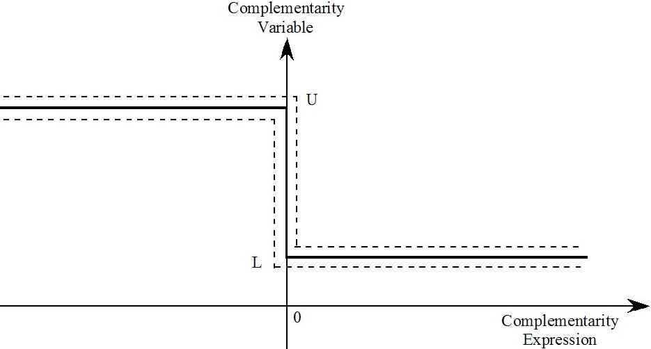
Figure 51.8 Whole plane divided into 3 (inexact) states
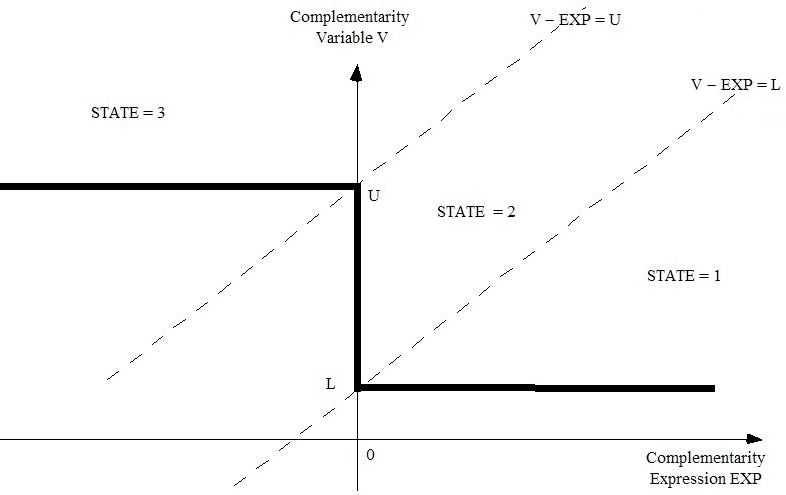
51.8 Complementarity examples [gpd3.16.8]
This section introduces several different models containing complementarities. The associated examples files are supplied with GEMPACK in the EXAMPLES subdirectory.
Examples on import quotas and tariff-rate quotas with Miniature ORANI (sections 51.8.1 to 51.8.3 below) are in the zip file MOQ.ZIP.
GTAP examples on bilateral tariff-rate quotas and global tariff-rate quotas (sections 51.8.4 to 51.8.6 below) are in G5TRQ.ZIP.
G94-QUO.ZIP contains examples from GTAP94 with bilateral import quotas and bilateral export quotas (see sections 51.8.7 and 51.8.8 below).
51.8.1 Example: MOIQ (miniature ORANI with import quotas) [gpd3.16.8.1]
The various files referred to here can be found in the file MOQ.ZIP which should be in the EXAMPLES subdirectory supplied with the GEMPACK software.
The files needed are
- MOIQ.TAB the TABLO Input file,
- MO.DAT the usual MO data file,
- MOIQ_RAT.DAT, the supplementary GEMPACK text data file containing import quota data,
- MOIQ1C.CMF, MOIQ1D.CMF, MOIQ1CX.CMF and MOIQ1DR.CMF - Command files for this model.
See sections 51.3.1 and 51.3.2 above for details about the TABLO code and the supplementary data file MOIQ_RAT.DAT, and see section 51.4 above about running the first three of these example simulations and a discussion of results.
The Command file MOIQ1DR.CMF carries out the reversal of the MOIQ1D.CMF simulation.
Also supplied in MOQ.ZIP is TABLO Input file MOI2.TAB. This contains an alternative form of the Complementarity statement to implement an import quota. [The Complementarity statement in MOT2.TAB has an upper bound whereas the Complementarity statement in MOIQ.TAB has a lower bound.] Command files MOI21C.CMF, MOI21D.CMF and MOI21DR.CMF carry out simulations with MOI2.TAB. The results of these are the same as the corresponding simulations based on MOIQ.TAB (as you can check if you carry them out).
51.8.2 Example: MOTRQ (miniature ORANI with tariff-rate quotas) [gpd3.16.8.2]
The various files referred to here can be found in the file MOQ.ZIP which should be in the EXAMPLES subdirectory supplied with the GEMPACK software.
The files needed are:
- MOTRQ.TAB, the TABLO Input file. This is usual Miniature ORANI TABLO Input file MO.TAB with tariff-rate quotas added.
- MO.DAT, the usual data file for MO.
- MOTRQ.DAT, a test data file which contains supplementary data for tariff-rate quotas.
- MOTQ1C.CMF, MOTQ1D.CMF and MOTQ1DR.CMF - the Command files for this model.
Associated with a tariff-rate quota are two import tariff rates. The lower rate (the in-quota rate) applies when the import volume is below the quota volume and the higher rate (the over-quota rate) applies when the import volume exceeds the quota volume.
Suppose by way of example, that the ad valorem in-quota rate is 25% and that the ad valorem over-quota rate is 400%. Then the in-quota power of the tariff is 1.25 and the over-quota power of the tariff is 5.
When the import volume is exactly equal to the quota volume, the tariff rate (the on-quota rate) is somewhere between the in-quota rate and the over-quota rate. Import volumes do not exceed the quota volume until importers are prepared to pay the full over-quota rate. As economic conditions become more favourable towards imports, the on-quota rate increases from the in-quota rate towards the over-quota rate. If conditions become extremely favourable to imports, the in-quota rate may rise to be equal to the over-quota rate, and then imports may expand to exceed the quota volume13.
In the numerical example above, the ad valorem on-quota rate varies between 25% and 400%.
MOTRQ.TAB
It is convenient to consider also the extra power of the import tariff due to the tariff-rate quota. In the TAB file MOTRQ.TAB you can see the following levels variables declared.
Variable (all,i,COM) TIMP(i) # power of import duty # ! One plus rate of import duty on commodity 1 - DPSV t(i) ! ; (all,i,COM) XIMP(i) # import quantities # ; (GT 0) (all,i,COM) XIMP_TRQ(i) # TRQ quota volume # ; (GT 0) (all,i,COM) TIMP_INQ(i) # in-quota power of import tariff # ; (all,i,COM) TIMP_TRQOVQ(i) # extra power of import tariff in over-quota case # ; (GT 0) (all,i,COM) TIMP_OVQ(i) # total power of import tariff in over-quota case # ; (GT 0) (all,i,COM) TIMP_TRQ(i) # actual extra power of import tariff due to TRQ # ; (GE 0, LE 1) (all,i,COM) XIMP_RATIO(i) # Current volume [XIMP] divided by TRQ quota volume [XIMP_TRQ] # ;
This makes the distinction between the total power of the import tariff in the over-quota case TIMP_OVQ(i) and the extra power of the import tariff in the over-quota case TIMP_TRQOVQ(i). These are connected by the equation.
Formula & Equation E_TIMP_OVQ # Total power in over-quota case # (All,i,COM) TIMP_OVQ(i) = TIMP_INQ(i) * TIMP_TRQOVQ(i) ;
In the numerical example above (where the in-quota power is 1.25 and the over-quota power is 5), TIMP_INQ is 1.25, TIMP_OVQ is 5 and so the extra power TIMP_TRQOVQ is 4 and the equation above says that 5 = 1.25*4.
There is also the distinction between the actual power of the import tariff TIMP(i) and the extra power due to the tariff-rate quota TIMP_TRQ(i). These are related by the equation.
Formula & Equation E_TIMP_TRQ # Actual extra power due to TRQ # (All,i,COM) TIMP_TRQ(i) = TIMP(i)/TIMP_INQ(i) ;
In the numerical example above, the actual power of the tariff TIMP can vary between 1.25 and 5. The extra power of the tariff due to the tariff-rate quota TIMP_TRQ can vary between 1 and 4.
The complementarity statement in MOTRQ.TAB is.
COMPLEMENTARITY
(Variable = TIMP_TRQ,
Lower_Bound = 1,
Upper_Bound = TIMP_TRQOVQ) TRQ
(All,i,COM) 1 - XIMP_RATIO(i) ;
The complementarity variable is TIMP_TRQ, the extra power of the import tariff due to the tariff-rate quota.
The complementarity expression is 1 - XIMP_RATIO(i), where
XIMP_RATIO(i) = XIMP(i) / XIMP_TRQ(i)
is the ratio between the current volume of imports XIMP(i) and the TRQ quota volume XIMP_TRQ(i).
Supplementary TRQ Data in File MOTRQ.DAT
The supplementary data are in the text data file MOTRQ.DAT. These data imply that
- imports of both commodities are in-quota.
- imports of commodity 1 are 0.75 of the quota volume while .imports of commodity 2 are 0.8 of the quota volume.
- the full extra power of the import tariff due to the tariff-rate quota is 4.0 for each commodity. That is, if imports of either commodity exceed the quota volume, this extra power of the tariff will apply.
You might like to examine MOTRQ.DAT in your text editor to see the actual data held there. The relevant levels variables and read statements in the TAB file are shown below.
Variable (GE 0) (all,i,COM) VIMP_TRQ(i) # value of quota volume at world prices (foreign currency) # ; (GE 0) (all,i,COM) VIMPINQ_TRQ(i) # value of quota volume at in-quota prices (foreign currency) # ; !---------------------------------------------------------------! ! Extra READs for Tariff-Rate Quotas ! !---------------------------------------------------------------! FILE (TEXT) trq_data # Text file containing TRQ data # ; READ TIMP_TRQOVQ FROM FILE trq_data ; READ VIMP_TRQ FROM FILE trq_data ; READ VIMPINQ_TRQ FROM FILE trq_data ;
The values of imports at world prices (as shown in the standard data file MO.DAT for Miniature ORANI) are 9 and 12 for the two commodities. [The total values including duty are 10 and 17, as seen from headers "IIMP" and "IMPH", while duty values are 1 and 5 respectively — see header "DUTY".] The VIMP_TRQ values on MOTRQ.DAT are 12 and 15 respectively. These mean that the corresponding XIMP_RATIO values are 0.75 (=9/12) and 0.8 (=12/15) respectively since.
XIMP_RATIO(i) = XIMP(i)/XIMP_TRQ(i) = VIMP(i)/VIMP_TRQ(i)
[where VIMP(i) is the value of imports at world prices] because the common price PIMP(i) cancels out.
Since these XIMP_RATIO values imply that imports are in-quota in each case, the VIMPINQ_TRQ(i) values shown must be 10/0.75 and 17/0.8 respectively, since 10 and 17 are the values including duty.
This explains the values you see on MOTRQ.DAT.
Example Simulations with MOTRQ
(i) Decreasing the Quota Volume until imports are on-quota - MOTQ1C.CMF
The simulation in Command file MOTQ1C.CMF decreases the quota volume XIMP_TRQ("c1") for commodity 1 by 30%. After this shock, the quota volume will only be 70% as large as it was initially.
Since initial imports XIMP("c1") are 0.75 of the initial quota volume, after this decrease in the quota volume, you would expect imports of commodity 1 to be on (or over) quota.
If you run the simulation you will see indeed that imports of commodity 1 end up on-quota. The post-sim value of TIMP_TRQ("c1") is 1.116 (which is between its lower bound of 1 and the upper bound of 4).
Run the simulation14. Then open the Solution file MOTQ1C.SL4 in AnalyseGE. Right-click on the COMPLEMENTARITY statement and select Show State and Variable Values.
| STATE-PRE | STATE-POST | VAR-PRE | VAR-POST | EXP-PRE | EXP-POST | LB-PRE | LB-POST | UB-PRE | UB-POST | |
| c1 | 1 | 2 | 1 | 1.116 | 0.25 | 0 | 1 | 1 | 4 | 4 |
| c2 | 1 | 1 | 1 | 1 | 0.2 | 0.177 | 1 | 1 | 4 | 4 |
The table shows that for commodity 1, the pre-sim value of the complementarity variable (VAR-PRE) is 1.0 and expression (EXP-PRE) is 0.25. Both values are consistent with commodity 1 being in-quota (that is, in state 1 — see the STATE-PRE column in the table). It shows that the post-sim value of the complementarity variable (VAR-POST) and expression (EXP-POST) for commodity 1 are 1.116 and 0.0 respectively. Both values are consistent with commodity 1 being on-quota after the simulation (that is, in state 2 — see the STATE-POST column in the table). This table also shows that the value of the complementarity expression for commodity 2 has decreased from 0.2 (pre-sim) to 0.177 (post-sim). Thus imports of commodity 2 increase in volume but remain in-quota.
It is also instructive to look at the updated supplementary TRQ data in file MOTQ1CQ.UPD. The extra powers of the tariff for over-quota imports do not change - they remain equal to 4.0 for each commodity. But the values of VIMP_TRQ and VIMPINQ_TRQ change for commodity 1. These are the values of the quota volume valued firstly at world prices (VIMP_TRQ) and secondly at the in-quota tariff rate (VIMPINQ_TRQ). Both are held in foreign dollars. For commodity 1 these are reduced by 30% (since the quota volume for commodity 1 has been reduced by 30% and foreign currency prices have not changed). These values for commodity 2 are unchanged since the quota volume and the foreign currency price is unchanged.
If you look at the log file motq1c.log produced in this run, you can see when the state change occurs during the approximate run. [Search for the word state in the log file.] You should find that the state for commodity c1 changes from 1 (in-quota) to 2 (on-quota) during Euler step 17 of the approximate run15. You can also see a little further down the log file that this step 17 is redone with a shorter length (see section 51.7.3).
(ii) Decreasing the Quota until the imports are over quota - MOTQ1D.CMF
The simulation in Command file MOTQ1D.CMF decreases the quota volume XIMP_TRQ("c1") for commodity 1 by 70%. This is a larger decrease than in MOTQ1C.CMF.
If you run the simulation you will see that imports of commodity 1 end up over-quota. The post-sim value of TIMP_TRQ("c1") is 4.000 and the post-sim value of the complementarity expression is .0.2678. Both of these values are consistent with commodity 2 being over-quota (since 4.0 is the full extra power of the import tariff which applies to over-quota imports of commodity 1 - see MOTRQ.DAT). [Again you can see these values most easily if you use AnalyseGE.]
The post-sim state of commodity 2 is interesting. You can see from AnalyseGE that this commodity ends up on-quota. Imports of this commodity expand and the post-sim values of the complementarity variable and expression for this commodity are 1.502 and 0.0 respectively.
Again it is instructive to look at the updated supplementary TRQ data in file MOTQ1DQ.UPD.
(iii) Increasing the Quota Volume MOTQ1DR.CMF - Reversing MOTQ1D
In MOTQ1D.CMF the quota volume for commodity 1 was decreased by 70%. The reversal of this in the Command file MOTQIDR.CMF is to increase the quota volume for this commodity by 233.333%16.
This simulation starts from the updated data after the MOTQ1D simulation. The shock is a 233.333% increase in the quota volume for commodity 1. You would expect the results of this simulation to be the exact opposite of the results of the original MOTQ1D simulation. And you would expect the post-simulation data after this reversal to be the same as the original MO data and supplementary TRQ data. It is easy to check these expectations, as we explain below.
For the simulation results, consider two examples.
(i) Look at industry activity in the first sector, that is p_Z("c1"). The result in MOTQ1D is a decrease of 13.749372%17. The reversal of such a decrease is an increase of 15.9412% 18.
The results from the reversal simulation MOTQ1DR show an increase of 15.9337% which is acceptably close to 15.9412.
(ii) Look at changes in import volumes p_XIMP for the two commodities. The MOTQ1D results show a decrease of 49.280865% in imports of commodity 1 and an increase of 25.0% in imports of commodity 2.. The exact reversals of these would be an increase of 97.1642% for commodity 1 and a decrease of 20.0% for commodity 219. The simulation results from MOTQ1DR indicate an increase of 97.1801% for commodity 1 and a decrease of 19.997% for commodity 2. Again these are reasonably close to the exact results. [Of course, you could get even better agreement if you carried out both simulations more accurately - that is, took more Gragg steps.]
For the data, you can use the GEMPACK program CMPHAR (see section 37.2) to compare the post-simulation data MOTQ1DR.UPD after the reversal simulation with the original data MO.DAT. You will find that they agree to at least 3-4 figures. You should also compare the supplementary TRQ data, that is compare MOTQ1DRQ.UPD with the original MOTRQ.DAT. [These are both text files.] Again you will find good agreement.
51.8.3 Example: MOTR2 (alternative COMPLEMENTARITY statement) [gpd3.16.8.3]
MOTR2.TAB is the same as MOTRQ.TAB except that an alternative form of the COMPLEMENTARITY statement is used.
COMPLEMENTARITY
(Variable = TIMP,
Lower_Bound = TIMP_INQ,
Upper_Bound = TIMP_OVQ) TRQ2
(All,i,COM) 1 - XIMP_RATIO(i) ;
In this alternative form, the complementarity variable is TIMP, the actual power of the import tariff. The lower and upper bounds are accordingly different from those in MOTRQ.TAB. In MOTR2.TAB the lower bound is TIMP_INQ (the in-quota power of the tariff) and the upper bound is TIMP_OVQ (the power of the tariff which applies if imports are over-quota).
The complementarity expression is the same as in MOTRQ.TAB.
Example Simulations with MOTR2 - MOT21C.CMF and MOT21D.CMF
These are very similar to the corresponding cases for MOTRQ.TAB You should run them and compare the results with those using MOTRQ.TAB. [First use AnalyseGE to look at the pre-sim and post-sim values of the complementarity variable and expression. Then look at some simulation results via ViewSOL.]
51.8.4 Example: G5BTRQ (GTAP with bilateral tariff-rate quotas) [gpd3.16.8.4]
The various files referred to here can be found in the file G5TRQ.ZIP which should be in the EXAMPLES subdirectory supplied with the GEMPACK software.
The files needed are:
- G5BTRQ.TAB, the TABLO Input file for GTAP with bilateral tariff-rate quotas.
- G5BTRQ.STI the condensation file for G5BTRQ.TAB .
- Standard data files for GTAP, SET6x4v5.HAR, DAT6x4v5.HAR and PAR6x4v5.HAR .
- Extra files with Bilateral TRQ data, TRQ6x4v5.HAR and QSHR6x4.DAT .
- 1A5.CMF and 1B5.CMF, two of the Command files for this model.
A brief introduction to tariff-rate quotas can be found in section 51.8.2 above. Further background information can be found in GTAP Technical Paper No 18 [Elbehri and Pearson (2000)], which we refer to here as TP18].
G5BTRQ.TAB
This TAB file is very similar to the file GTAP5TRQ.TAB described in TP18.
In G5BTRQ.TAB, a COMPLEMEMNTARITY statement is used to specify the behaviour required for bilateral tariff-rate quotas. The COMPLEMENTARITY statement in G5BTRQ.TAB is
COMPLEMENTARITY
(Variable = TMSTRQ,
Lower_Bound = 1,
Upper_Bound = TMSTRQOVQ) TRQ
(All,i,TRAD_COMM)(All,r,REG)(All,s,REG)
1 - QXSTRQ_RATIO(i,r,s) ; ! The complementarity expression !
This Complementarity means:
| Either | TMSTRQ = 1 | and | 1 - QXSTRQ_RATIO > 0 | [in-quota], |
| or | 1 <= TMSTRQ <= TMSTRQOVQ | and | 1 - QXSTRQ_RATIO = 0 | [on-quota], |
| or | TMSTRQ = TMSTRQOVQ | and | 1 - QXSTRQ_RATIO < 0 | [over-quota] |
The condensation Stored-input file G5BTRQ.STI (for running TABLO) is supplied in G5TRQ.ZIP. You can switch between GEMSIM and TABLO-generated program output by switching between "pgs" and "wfp" near the end of this Stored-input file.
The "B" in the name of this stands for "Bilateral" to distinguish this from the Global TRQ case (where "G" is used — see section 51.8.6 below).
51.8.4.1 Connections Between Complementarity and Rest of TAB File [gpd3.16.8.4.2]
We have built G5BTRQ.TAB by adding a module to a standard version of the TABLO Input file GTAP.TAB for the GTAP model. In fact G5BTRQ.TAB is based on Version 5.0 (May 2000) of GTAP.TAB since that was the version of GTAP.TAB used as the basis of the TABLO Input files in TP18. In G5BTRQ.TAB, the TRQ module is added after the basic GTAP model and before the Welfare Decomposition and Terms of Trade modules. The TRQ module added to Version 5.0 of GTAP.TAB could easily be added to the current version of GTAP.TAB (Version 6.1, August 2001). Few, if any, changes would be needed.
As explained earlier (see section 51.3.5), a COMPLEMENTARITY statement must be expressed using levels variables. This may seem to be a problem when the COMPLEMENTARITY statement is being added at the end of a TAB file such as GTAP.TAB in which there are mainly (or exclusively) linear variables (changes and percentage changes) and very few (if any) levels variables.
This problem is easily solved, as we explain here. The idea is to add levels variables whose linearized versions are equal to linearized variables already in the model, and to add equations which link the two together (see also section 11.14.2).
This is best explained and understood in the context of a concrete example. We describe below a couple of these linking equations from G5BTRQ.TAB.
One of the important relations is:
TMS(i,r,s) = TMSTRQ(i,r,s) * TMSINQ(i,r,s)
Since TMSTRQ and TMSINQ are introduced in the TRQ module as levels variables, it is natural to want to write this down as a levels equation. But in the GTAP.TAB being added to, the variable tms appears only as a linear, percentage-change variable, not as a levels variable. Introducing a levels version (which we call TMS_L to distinguish it from the "tms" already in GTAP.TAB) is done as follows:
VARIABLE (Levels, Linear_var = tms)
(all,i,TRAD_COMM)(all,r,REG)(all,s,REG) TMS_L(i,r,s)
# Total import tariff for TRQ commodity i from r into s. # ;
Formula (Initial) (all,i,TRAD_COMM)(all,r,REG)(all,s,REG)
TMS_L(i,r,s) = VIMS(i,r,s)/VIWS(i,r,s) ;
Formula & Equation E_TMSTRQ (all,i,TRAD_COMM)(all,r,REG)(all,s,REG)
TMSTRQ(i,r,s) = TMS_L(i,r,s) / TMSINQ(i,r,s) ;
The "Linear_var=tms" qualifier (see sections 9.2.2 and 10.4) in the declaration of the new levels variable TMS_L indicates that the linear variable associated with TMS_L is just the variable tms which is already in the model. [That is, the variable tms indicates the percentage change in TMS_L.]
The initial values for TMS_L are set up via the Formula(Initial) shown. The link between the levels variables TMS_L, TMSINQ and TMSOVQ is made via the final Formula & Equation shown. This is written as shown since the Formula part is used to give the pre-simulation values for TMSTRQ.
Note that, prior to the introduction of the LINEAR_VAR= qualifier, the connection between the new levels variable TMS_L and the linear variable tms already in the TAB file would have been made as follows.
VARIABLE (levels) (all,i,TRAD_COMM)(all,r,REG)(all,s,REG) TMS_L(i,r,s) # Total import tariff for TRQ commodity i from r into s. # ; Equation (Linear) E_TMS_L (all,i,TRAD_COMM)(all,r,REG)(all,s,REG) p_TMS_L(i,r,s) = tms(i,r,s) ;
The declaration of TMS_L here automatically generates the associated percentage-change linear variable p_TMS_L (see section 9.2.2). The equation E_TMS_L says that p_TMS_L and tms are the same. [If you look in GTAP5TRQ.TAB in Elbehri and Pearson (2000), you will find these equations since that TAB file was written while Release 7.0 of GEMPACK was current. At that time, LINEAR_VAR= qualifiers were not available.] We strongly recommend that you use LINEAR_VAR= qualifiers to simplify linking code.
If you look in G5BTRQ.TAB near the start of the Tariff-Rate Quota module added at the end, you will see other linking equations.
The general procedure for providing equations to link a levels module (at the end of a TAB file) to a linear model is also described in detail in Harrison and Pearson (2002), "Adding Accounting-Related Behaviour to a Model Implemented Using GEMPACK".
Example Simulations with G5BTRQ
Any of the example simulations and applications described in TP18 could be carried out using G5BTRQ. We refer you to that Technical Paper for more details about these simulations, the rationale behind them and the construction of the starting data base.
We have supplied Command files for several example simulations with G5BTRQ.TAB. We discuss these briefly below.
We encourage you to carry out all of these simulations if you are interested in modelling tariff-rate quotas.
Checking the Simulation Results
When you carry out one of these simulations, you should check the results in much the same way as you checked the results of the simulations in sections 51.4 and 51.8.2 above. In particular,
- use AnalyseGE to look at the pre-sim and post-sim states and values of the complementarity variables and expressions.
- look at the log file to follow through the state changes during the approximate run and to look at the other state reports. We give a detailed example of this in section 51.8.4 below.
- look at the updated data (especially the updated supplementary TRQ data) to check that the values there are consistent with the post-simulation states.
When checking a reversal simulation (for example, 1A5R.CMF and 1B5R.CMF), you should follow the methods described in the discussion of the reversal MOTQ1DR.CMF simulation in section 51.8.2 above to check that
- states and values of complementarity variables and expressions return to their original value.
- simulation results are reversed
- the updated data after the reversal simulation is essentially identical to the data before the original simulation.
Increasing the In-quota Tariff - Command files 1A5.CMF and 1B5.CMF
These are simulations in which the in-quota tariff on sugar imported from Africa (AFR) to the United States (USA) is increased. These are what are called Cases 1A and 1B in TP18. In 1B5, the triple (sugar,AFR,USA) moves from state 3 (over-quota) to state 1 (in-quota).
Reversals - Command files 1A5R.CMF and 1B5R.CMF
The reversal 1B5R.CMF of case 1B is especially interesting. The shock in the Case 1B simulation is relatively large (a doubling of the in-quota tariff for sugar from AFR to USA) so this simulation is relatively nonlinear. Accordingly the reversal simulation has to "work quite hard" to get back to the original (that is, before Case 1B is run) over-quota state 3. This is especially so since the original state of (sugar,AFR,USA)20 is over quota (state 3) but not all that far over quota since the original import volume is 1.057 times the quota volume.
If you try the reversal 1B5R.CMF with 20 steps in the approximate run, the reversal simulation fails (even though the accurate run converges well). [To carry out 1B5R with just 20 Euler steps, change the relevant statement in 1B5R.CMF to "complementarity steps_approx_run = 20 ;".] The LOG file shows various problems. The most obvious ones are that, at the end of the accurate run,
the post-simulation value of TMSTRQ(sugar,AFR,USA) is 1.844 which exceeds the upper bound of 1.8199 [the value of TMSTRQOVQ(sugar,AFR,USA)] specified in the COMPLEMENTARITY statement.
the post-sim state for triple (sugar,AFR,USA) is 2 (on-quota) after the approximate run while it is 3 (over-quota) after the accurate run.
Thus the simulation fails with 20 Euler steps. Similar problems occur if you take 40 Euler steps (when again the post-sim state for (sugar,AFR,USA) is 2 after the approximate run instead of the desired state 3). However these problems all disappear if you take 50 Euler steps.
Reversal of 1B5 with Automatic Accuracy - Command file 1B5RAA.CMF
Having to reach the correct post-sim state in a relatively nonlinear simulation like this in a single Euler calculation is quite demanding. It is for this reason that it may be better to allow the software to break the simulations (approximate and accurate) into several subintervals (of possibly different lengths). This is what happens with user-specified accuracy, which you have when you put the statement "automatic accuracy = yes ;" in your Command file (see section 51.7.4 for more details). You can see the effects of this if you carry out the reversal simulation using Command file 1B5RAA.CMF. [In this, only 20 Euler steps are specified for the approximate run. The software takes 2 subintervals, each taking 20 Euler steps for the approximate run, to complete the run. Although the total CPU time may be greater than for a single subinterval with 50 Euler steps in the approximate run, you may waste a lot of time experimenting before you realise that 50 steps are required in that case.]
Reversal of 1B5 with Automatic Accuracy again - Command file 1B5RAAX.CMF
This is the same as 1B5RAA.CMF except that one subinterval is specified to start with. The attempt to do the whole simulation in one subinterval fails because the post-sim state for (sugar,AFR,USA) is 3 after the accurate simulation but 2 after the approximate simulation. The subinterval length is reduced and the simulation then proceeds ok.
Reporting State Changes - Command file 1B5.CMF
Whenever you carry out a simulation in which one or more complementarities may change state, you should check the state changes, as reported in the log file of the run. We illustrate this below by following through in detail the reports about states and state changes in the log file from the 1B5.CMF simulation. [You can do the same for the other simulations with this and other models involving complementarities.]
In this simulation, the in-quota power of the tariff on (sugar,AFR,USA) is doubled and the ratio between over-quota and in-quota powers remains fixed. This moves the triple (sugar,AFR,USA) from over-quota to in-quota.
There are 20 Euler steps in the initial approximate simulation followed by an accurate simulation using the Gragg method with 8, 12, 16 steps:
Method = Gragg ; Steps = 8 12 16 ; complementarity steps_approx_run = 20 ;
[The "steps_approx_run" statement is a way of telling the software how many Euler steps to take in the approximate run. It is optional. See section 51.6 for more details.]
It is instructive to follow the state changes reported during this run.
In the log file 1b5.log from this run, you can see the approximate run (a 20-step Euler). At the beginning the program reports that 136 of the 144 triples (i,r,s). are in state 1 (in-quota) and that 8 are in state 3 (over quota). During step 1 of the 20 Euler steps, the program reports that (sugar,AFR,USA) moved from state 3 to state 2 (on quota). During step 16 it reports that (sugar,AFR,USA) moved from state 2 to state 1. After the approximate run it tells you that 1 triple moved from state 3 to state 1 and that the other 143 remained in their pre-simulation states.
[To see the state reports, search for "state" in the log file.]
The pre-simulation state report is as follows:
[Complementarity TRQ. Numbers initially in states. 1, 2 and 3 are 136, 0 and 8 respectively.]
The program will report changes in state as they occur throughout the approximate simulation. For example, there is a state change from state 3 to state 2 during Euler step number 1, as reported below:
[Complementarity TRQ("Sugar","AFR","USA"):
State change from 3 to 2 during this step.
Occurs after 0.25966060 part of the step.]
(Redoing this step to change state more gradually.)
Whenever a state change occurs during a step, the step is repeated with a shorter step length to ensure that the state change occurs near the end of this (shorter) step. [The reasons for this are set out in section 51.7.3.] Because of the above state change during step 1, this step is carried out again. The state change report in this repeated step is as follows:
[Complementarity TRQ("Sugar","AFR","USA"):
State change from 3 to 2 during this step.
Occurs after 0.99961501 part of the step.]
Then later there is another state change from state 2 to state 1 during Euler step 17:
---> Beginning pass number 17 of 20-pass calculation.
[Complementarity TRQ("Sugar","AFR","USA"):
State change from 2 to 1 during this step.
Occurs after 0.79648900 part of the step.]
(Redoing this step to change state more gradually.)
This step is also repeated (with a shorter length). The reported state change during this repeated step number 17 is:
(Beginning the update after pass 17 of this 20-pass calculation.)
[Complementarity TRQ("Sugar","AFR","USA"):
State change from 2 to 1 during this step.
Occurs after 0.99987364 part of the step.]
At the end of the approximate simulation just before starting the accurate Gragg simulation there is a report of state changes which occurred during the approximate run, and which are therefore expected during the accurate simulation :
===> Beginning accurate complementarity calculation.
[Processing complementarity TRQ.]
[Are 0 changing from state 1 to state 2, and
0 changing from state 1 to state 3.]
[Are 0 changing from state 2 to state 1, and
0 changing from state 2 to state 3.]
[Are 1 changing from state 3 to state 1, and
0 changing from state 3 to state 2.]
[Numbers remaining unchanged in states 1,2 and 3 are
136, 0 and 7 respectively.]
[Total numbers in post-sim states 1,2 and 3 are
137, 0 and 7 respectively.]
---> Beginning pass number 1 of 9-pass calculation.
51.8.5 Alternative form of the complementarity - G5BTR2.TAB [gpd3.16.8.5]
The files needed are:
- G5BTR2.TAB, the TABLO Input file for GTAP with Bilateral Tariff-Rate Quotas.
- G5BTR2.STI the condensation file for G5BTRQ.TAB .
- Standard data files for GTAP, SET6x4v5.HAR, DAT6x4v5.HAR and PAR6x4v5.HAR .
- Extra files with Bilateral TRQ data, TRQ6x4v5.HAR and QSHR6x4.DAT .
The Command files for the G5BTRQ model can be used with this model by changing the name of the auxiliary files to g5btrq2 instead of g5btrq.
This TAB file is the same as G5BTRQ.TAB except that an alternative form of the complementarity statement is used. This version has TMS_L [the levels value of the actual total import tariff (including any due to the tariff-rate quota)] as the complementarity variable instead of TMSTRQ (the extra power of the tariff due to the tariff-rate quota). The lower and upper bounds in this second case are TMSINQ (the in-quota power) and TMSOVQ (the total over-quota power) respectively. The complementarity statement in G5BTR2.TAB is:
COMPLEMENTARITY (Variable = TMS_L,
(Lower_Bound = TMSINQ, Upper_Bound = TMSOVQ) TRQ2
(All,i,TRAD_COMM)(All,r,REG)(All,s,REG)
1 - QXSTRQ_RATIO(i,r,s) ; ! The complementarity expression !
This second form of the complementarity means:
| Either | TMS_L = TMSINQ | and | 1 - QXSTRQ_RATIO > 0 | [in-quota], |
| or | 1 <= TMS_L <= TMSOVQ | and | 1 - QXSTRQ_RATIO = 0 | [on-quota], |
| or | TMS_L = TMSOVQ | and | 1 - QXSTRQ_RATIO < 0 | [over-quota] |
The condensation Stored-input file G5BTR2.STI (for running TABLO) is supplied in G5TRQ.ZIP. You can switch between GEMSIM and TABLO-generated program output by switching between "pgs" and "wfp" near the end of this Stored-input file.
Example Simulations with G5BTR2
Any of the simulations with G5BTRQ.TAB can be carried out with G5BTR2.TAB. We supply only the Command file 1B5R2.CMF carries out the reversal of Case 1B (see section 51.8.4 above) using G5BTR2.TAB instead of G5BTRQ.TAB.
We suggest that you carry out the 1B5R2.CMF simulation and check that the results are the same as for the 1B5R.CMF simulation which is based on G5BTRQ.TAB.
In this reversal 1B5R2.CMF simulation, the post-simulation state of the triple (sugar,AFR,USA) is 3 (over-quota). Thus, in the accurate simulation, the complementarity variable must be shocked so that it becomes equal to the upper bound. With the alternative form of the complementarity in G5BTR2.TAB (see above), the upper bound TMSOVQ is endogenous. Hence this is an example where the variable TRQ2@U (set equal to the difference between the complementarity variable TMS_L and the upper bound — see Case 3(b) in section 51.7.1) is made exogenous and shocked (to zero).
51.8.6 Example: G5GTRQ (GTAP with global and bilateral trqs) [gpd3.16.8.6]
With a bilateral TRQ, the trigger is the bilateral import volume. In contrast, a global TRQ is one which is triggered by aggregate imports (from all exporting regions).
The files needed are:
- G5GTRQ.TAB, the TABLO Input file for GTAP with global and bilateral tariff-rate quotas.
- G5GTRQ.STI the condensation file for G5GTRQ.TAB .
- Standard data files for GTAP, SET6x4v5.HAR, DAT6x4v5.HAR and PAR6x4v5.HAR .
- Extra file with supplementary global TRQ data, GTRQ6x4.DAT .
In G5GTRQ.TAB is a
- bilateral TRQ for commodity sugar, and
- a global TRQ for commodity othag (other agriculture).
[It would be easy to modify this TAB file to apply to different commodities.]
You may like to look in G5GTRQ.TAB to see how the global TRQ is specified.
In the supplementary global TRQ data supplied (see file GTRQ6X4.DAT), imports of othag into the 4 regions ASI (Asia), LAM (Latin America), AFR (Africa) and ROW (Rest-of-World) are over quota while imports into the remaining 2 regions USA and E_U (Europe) are in quota. The full extra power of the tariff TMTRQOVQ due to the global TRQ is 8.0 for USA and E_U and is 1.4 for the other 4 regions. Imports into USA and E_U are assumed to be 0.8 of the quota volume while imports into the other 4 regions are assumed to be 1.2 times the quota volume.
The condensation Stored-input file G5GTRQ.STI (for running TABLO) is supplied in G5TRQ.ZIP. You can switch between GEMSIM and TABLO-generated program output by switching between "pgs" and "wfp" near the end of this Stored-input file.
The "G" in the name of this stands for "Global" to distinguish this from the Bilateral TRQ case (where "B" is used — see section 51.8.4 above).
Example Simulations with G5GTRQ
Below we describe briefly the example simulations provided with the GEMPACK examples.
We suggest that you carry out all these simulations and that you check the results following the general guidelines given above under the heading "Checking the Simulation Results" in section 51.8.4.
Bilateral and Global TRQ combined - Command file G2B5.CMF
In this Command file, the Case 1B bilateral TRQ shock (see 1B5.CMF above) is given. There is also a 25% increase in the global TRQ quota volume for imports of othag into Africa.
In the pre-simulation data, (othag,AFR) is in state 3 with respect to the global TRQ. The effect of these shocks is to bring (othag,AFR) on-quota with respect to the global TRQ and to bring (sugar,AFR,USA) in-quota with respect to the bilateral TRQ on sugar. If you carry out this simulation, you can see from the LOG file approximately when these state changes occur during the approximate run. The state changes for the whole simulation are reported at the end of the whole run.
You can find interesting information about the 2 complementarities via AnalyseGE.
Reversal of G2B5 - Command file G2B5R.CMF
As with 1B5R (see above), 40 Euler steps are not sufficient for the approximate run, but 50 steps are sufficient. [Again automatic accuracy would be a good option.]
When you check that the reversal has worked, and are looking to compare the updated data after the reversal simulation with the original data, you should remember to compare the supplementary data files as well as the main GTAP data file. For example, you should compare the updated supplementary global TRQ data in file G2B5RG.UPD with the original data in file GTRQ6X4.DAT (which you can do in a text editor since they are text files).
51.8.7 Example: G94-XQ (GTAP94 with bilateral export quotas) [gpd3.16.8.7]
The various files referred to here can be found in the file G94-QUO.ZIP which should be in the EXAMPLES subdirectory supplied with the GEMPACK software.
The files needed are:
- G94-XQ.TAB, the TABLO Input file for GTAP94 with bilateral export quotas.
- G94-XQ.STI the condensation file for G94-XQ.TAB .
- Standard data files for GTAP94, SET2-01.HAR, DAT2-01.HAR and PAR2-01.DAT .
- Extra file with supplementary data, XQ2-01.DAT .
- Command files XQ-A2.CMF, XQ-A4.CMF, XQ-A6.CMF and XQ-P2.CMF.
This example is supplied as an updated version of the bilateral export quota model and applications supplied with Bach and Pearson (1996) which is GTAP Technical Paper No. 4 [TP4]. The Technical Paper TP4 described an early implementation of bilateral export and import quotas with GTAP and GEMPACK.
Additional Export Quota Data XQ2-01.DAT
Extra data is required to indicate the pre-simulation state of the quotas. As in TP4, this extra data is for 3 tradeable commodities (food, manufactures, services) and three regions USA, EU and ROW. The extra quota data is set up so that no quotas are binding. Exports of manufactures "mnfcs" from ROW to USA and EU are 0.98 of the quota volume (that is, these two quotas are nearly binding). In all other cases, exports are 0.2 of the quota volume (that is, the quotas are far from binding).
In TP4 the extra data consisted of VXQD (values of exports by destination at prices which include normal export taxes or subsidies, but do not include the extra tax due to the quota) and QXS_RATIO values (the ratio of current export volume to the quota volume). In G94-XQ.TAB we have chosen to hold TXS_QUOTA (the extra power of the export tax due to the quota) instead of the VXQD values. Because no quotas are binding in this extra data, all TXS_QUOTA values are 1.
G94-XQ.TAB
This is version 2.2a (August 1995) of GTAP94.TAB with export quotas added. The TAB file statements to implement export quotas are at the end of that file. Similar (probably identical) statements could be added to more recent versions of GTAP.TAB to do the same job.
The export quota module in G94-XQ.TAB file is shown below. Noteworthy features are:
- Only two levels variables TXS_QUOTA and QXS_RATIO are added for the complementarity. These must be levels variables because the COMPLEMENTARITY statement requires levels variables (see section 51.3.5).
- The only other variables required to link to the rest of the model are qxs_quota and pxs. Each of these has been added as a linear (percentage-change) variable [although these could have been added as levels variables].
- The accounting identities linking prices and ratios have been put in as Linear equations called E_QXS_RATIO and E_PFOB.
- The EXPRICES equation from the standard model must be altered as shown. [The version in the top of the file has been commented out.]
- The choice of which extra quota-related data to read (see section 51.8.7) affects the way the equations are written down. [If VXQD were read, as in TP4, probably some extra levels prices would have been needed.]
- Having only two new levels variables means that the code to link the quota code to the rest of the model (see section 11.14.2 and section 51.3.5 above) is extremely simple in this case.
Also shown below are the statements used to calculate and report the changes in the associated quota rents (see the equation E_QXS_RENT_RAT).
! Addition for export quotas in G94-XQ.TAB !
VARIABLE (Levels) (all,i,TRAD_COMM)(all,r,REG)(all,s,REG) TXS_QUOTA(i,r,s)
# extra export tax, due to quota, in r on good i bound for region s # ;
VARIABLE (Levels) (all,i,TRAD_COMM)(all,r,REG)(all,s,REG) QXS_RATIO(i,r,s)
# Ratio between volume of exports of i from r to s and import quota # ;
VARIABLE (Linear) (all,i,TRAD_COMM)(all,r,REG)(all,s,REG) qxs_quota(i,r,s)
# Volume export quota on exports of i from r to s # ;
VARIABLE (Linear) (all,i,TRAD_COMM)(all,r,REG)(all,s,REG) pxs(i,r,s)
# price of i supplied from r to s inclusive of normal export tariffs #;
! But exclusive of export quota tariff equivalents. May be less than
PMS(i,r,s) in the levels if the export quota on i from r to s is binding !
FILE (TEXT) EXP_QUOTA # File containing export quota data # ;
READ QXS_RATIO FROM FILE EXP_QUOTA ;
READ TXS_QUOTA FROM FILE EXP_QUOTA ;
Equation (Linear) E_QXS_RATIO # Links export volume, quota and ratio #
(all,i,TRAD_COMM)(all,r,REG)(all,s,REG)
! Levels equation is: QXS_RATIO=QXS_L/QXS_QUOTA !
qxs(i,r,s) = p_QXS_RATIO(i,r,s) + qxs_quota(i,r,s) ;
EQUATION (Linear) E_PFOB
# Links dom price of exports with usual and quota-related export tariffs #
(all,i,TRAD_COMM)(all,r,REG)(all,s,REG)
pfob(i,r,s) = pxs(i,r,s) + p_TXS_QUOTA(i,r,s) ;
! Next equations are modified from the usual GTAP94.TAB version
If this quota addition is used, the original equation (EXPRICES)
should be deleted or excluded with strong comment marks.
This equation links agent's and world prices. In addition to tx we have txs
which embodies both production taxes (all s) and export taxes (r not equal
to s) (HT#27)!
EQUATION EXPRICES (all,i,TRAD_COMM)(all,r,REG)(all,s,REG)
pxs(i,r,s) = pm(i,r) - tx(i,r) - txs(i,r,s) ;
COMPLEMENTARITY
(Variable = TXS_QUOTA, Lower_Bound = 1) EXPQUOTA
(all,i,TRAD_COMM)(all,r,REG)(all,s,REG) 1 - QXS_RATIO(i,r,s) ;
VARIABLE (Levels, Change)
(all,i,TRAD_COMM)(all,r,REG)(all,s,REG) QXS_RENT_RAT(i,r,s)
# Ratio of quota rent to pre-quota value of exports for each commodity #;
! Here pre-quota value is taken as the value including normal export
tariffs - that is, QXS_L*PXS_L.
Thus, in the levels,
QXS_RENT_RATIO_L= [QXS_L*(PFOB_L-PXS_L)]/[QXS_L*PXS_L]
= [PFOB_L/PXS_L] - 1
= TXS_QUOTA - 1 !
Equation (Levels) E_QXS_RENT_RAT (all,i,TRAD_COMM)(all,r,REG)(all,s,REG)
QXS_RENT_RAT(i,r,s) = TXS_QUOTA(i,r,s) - 1 ;
Example Simulations with G94-XQ
Those supplied are the accurate versions of the simulations XQ-A2.CMF, XQ-A4.CMF, XQ-A6.CMF and XQ-P2.CMF from TP4. All the same results as in TP4.
We suggest that you carry out all these simulations and that you check the results following the general guidelines given above under the heading "Checking the Simulation Results" in section 51.8.4.
We also suggest that you read the description of these simulations in TP4 and check that the results here are as reported there.
Decreasing the Quota - Command file XQ-A2.CMF
The shock in this simulation will reduces the quota for exports of mnfcs from ROW to USA. This makes it binding.
shock qxs_quota("mnfcs","ROW","USA") = -10;
Reversal of the XQ-A2.CMF Simulation - Command file XQ-A4.CMF
This simulation reverses the XQ-A2.CMF simulation.
shock qxs_quota("mnfcs","ROW","USA") = 11.111111 ;
Increase One Quota and Decrease Another Quota - Command file XQ-A6.CMF
This simulation starts from the post-simulation data after simulation XQ-A2. In simulation XQ-A2, the quota on (mnfcs,ROW,USA) was decreased by 10% which makes it binding.
The shocks in XQ-A6.CMF are to
- return the quota on (mnfcs,ROW,USA) to its original value (which should make it non-binding),
- decrease the quota on (mnfcs,ROW,EU) by 10 percent (which should make it binding).
It is instructive to look at the information which AnalyseGE provides if you right click on the COMPLEMENTARITY statement (in the TABmate form) and then select item Show State and Variable Values. If you select the drop-down boxes in the top right-hand corner of the ViewHAR form to show mnfcs, ROW, All REG, All $CPINFO respectively, you will see the following matrix (in which the row and column totals have been suppressed since they are of no value here).
| STATE-PRE | STATE-POST | VAR-PRE | VAR-POST | EXP-PRE | EXP-POST | LB-PRE | LB-POST | |
| USA | 2 | 1 | 1.037662 | 1 | 0 | 0.006597 | 1 | 1 |
| EU | 1 | 2 | 1 | 1.037282 | 0.007942 | 0 | 1 | 1 |
| ROW | 1 | 1 | 1 | 1 | 0.798572 | 0.798366 | 1 | 1 |
Look first at the USA row. This shows that the triple (mnfcs,ROW,USA) has changed from state 2 (STATE-PRE) where the quota is binding to state 1 (STATE-POST) where the quota is not binding. The values of the complementarity variable (TXS_QUOTA) confirm this. The pre-simulation value is 1.037662 (VAR-PRE) while the post-simulation value (VAR-POST) appears to be exactly 1. The values of the complementarity expression (1 - QXS_RATIO) also confirm this. The pre-simulation value (EXP-PRE) is exactly zero while the post-simulation value (EXP-POST) is 0.006597 which means that exports are approximately 0.993403 of the quota volume (that is, the quota is nearly binding). The last two columns (LB-PRE and LB-POST) shown the pre- and post-simulation values of the lower bound (both exactly 1).
You should also look at the EU and ROW rows. Check that all information in the EU row is consistent with the triple (mnfcs,ROW,EU) moving from non-binding to binding. Have exports of (mnfcs,ROW,ROW) moved closer to or further away from the (non-binding) quota?
51.8.8 Example: G94-IQ (GTAP94 with bilateral import quotas) [gpd3.16.8.8]
The various files referred to here can be found in the file G94-QUO.ZIP which should be in the EXAMPLES subdirectory supplied with the GEMPACK software.
This example is supplied as an updated version of the bilateral import quota model and applications supplied with Bach and Pearson (1996) which is GTAP Technical Paper No. 4 [TP4]. The Technical Paper TP4 described an early implementation of bilateral export and import quotas with GTAP and GEMPACK.
In TP4 bilateral import quotas are specified in the TAB file GTAP33IQ.TAB for all commodities, though the applications only relate to quotas on food imports. In G94-IQ.TAB the quotas are only specified for food (though it would be easy to add other commodities).
The files needed are:
- G94-IQ.TAB, the TABLO Input file for GTAP94 with bilateral import quotas.
- G94-IQ.STI the condensation file for G94-IQ.TAB .
- Standard data files for GTAP, SET2-01.HAR, DAT2-01.HAR and PAR2-01.DAT .
- Extra file with bilateral import data, IQ-FOOD.DAT .
- Command files IQ-B1.CMF and IQ-B3.CMF, also IQ-QUO1.CMF .
Additional Export Quota Data IQ-FOOD.DAT
Extra data is required to indicate the pre-simulation state of the quotas. As in TP4, this extra data is for 3 tradeable commodities (food, manufactures, services) and three regions USA, EU and ROW. The extra quota data is set up so that all quotas are just binding - that is, they bind but the extra power of the tariff due to the quotas is still 1.
In TP4 the extra data consisted of VIQS (values of imports by source at prices which include normal import taxes or subsidies, but do not include the extra tax due to the quota) and QIS_RATIO values (the ratio of current import volume to the quota volume). In G94-XQ.TAB we have chosen to hold TMS_QUOTA (the extra power of the import tax due to the quota) instead of the VIQS values. Because all quotas are just binding in this extra data, all TMS_QUOTA values are 1.
G94-IQ.TAB and Example Simulations
You may wish to look at the import quota implementation in G94-IQ.TAB. The relevant statements are near the bottom of the file. We have adopted a similar strategy to that in G94-XQ.TAB of adding the minimum number of levels variables in order to simplify the links with the rest of the model.
We suggest that you carry out all these simulations and that you check the results following the general guidelines given above under the heading "Checking the Simulation Results" in section 51.8.4.
We also suggest that you read the description of these simulations in TP4 and check that the results here are as reported there.
The applications IQ-B1.CMF and IQ-B3.CMF can be run with this model. All quotas start as binding which is classed as state 2 by the complementarity software. Because these quotas are just binding, there can be a large number of state changes at the start of any simulation (since a tiny move towards the quota being not binding will result in a state change). You can see these state changes if you look in the log files from these simulations.
In the IQ-B1.CMF simulation, the tariff on food imports of food from USA and ROW into EU is decreased. Since these quotas were originally binding, they remain binding. There are no quantity changes and the only price change is a 10% fall in the imported price (including normal import tariff but excluding the tariff equivalent of the import quota) of these two imports [this price is variable qis]. There is an increase in the associated quota rents as you can see from the c_QIS_RENT_RAT results.
In the IQ-B3.CMF simulation, as well as the tariff reductions in IQ-B1.CMF (see above), the quota volumes on imports of food from USA and ROW into the EU are increased by 15 percent. These quotas remain binding (and there is as associated increase in these two import volumes of 15 percent - the variable qxs). However the quotas on imports of food from ROW into USA and from EU into itself become non-binding, as you can see when you check the results.
We include another example, IQ-QUO1.CMF. In this example, quota volumes on food from both USA and ROW into EU are increased by 15 percent. Since all quotas are just binding in the pre-simulation data, the post-simulation equilibrium should be identical to the pre-simulation one except that these two quotas will be non-binding. Although not economically interesting, this simulation is interesting from a numerical point of view. After the approximate run, the post-simulation state for triple (food,EU,EU) is 1 (non-binding) whereas the state is 2 (binding) after the accurate run. Normally this would result in an error. But in this case, the software is able to tell that the post-simulation state after the accurate run (state 2) is also very close to state 1, so the software judges this to be ok. [In fact the post-sim state for this triple should be that the quota is just binding. It is somewhat arbitrary whether the software declares this to be state 1 or 2 since it is really on the corner in Figure 51.6.]
51.9 Piecewise linear functions via complementarities [gpd3.16.9]
In this section we show how various piecewise linear functions can be expressed accurately using Complementarity statements.
We begin with MAX and MIN. In view of section 51.3.6 above, it is not surprising that MAX and MIN can be expressed in terms of Complementarities.
We also include an example of a progressive income tax schedule in section 51.9.2. Other piecewise linear functions can be expressed similarly, as the examples in section 51.9.3 show.
51.9.1 Max and min [gpd3.16.9.1]
Z = MAX(0,Y)
Firstly consider the function Z = MAX(0,Y) [See Figure 51.9.]
This can be expressed via the Complementarity statement
COMPLEMENTARITY (Variable = Z, Lower_Bound = 0) <name> Z - Y ;
The Complementarity Variable is Z, the Lower Bound is zero and the Complementarity Expression is Z - Y.
To see this, suppose that Z = MAX(0,Y). Firstly note that Z >= 0 always so that 0 is a lower bound for Z. There are two cases:
(i) Suppose Y >= 0. Then Z=Y and so Expression Z - Y=0. Hence in this case, Variable Z >= Lower Bound 0 and Expression = 0. This is state 2 for the above Complementarity.
(ii) Suppose Y < 0. Then Z=0 so Variable is equal to Lower Bound. Also Expression Z - Y > 0. This is state 1 for the above Complementarity.
Z = MAX(X,Y)
| Firstly note that | Z = MAX(X,Y) |
| is the same as | Z - X = MAX(0,Y - X). |
We know from the section above how to express MAX(0,Y - X) using a Complementarity statement. Hence Z = MAX(X,Y) can be expressed using an equation to introduce variable W=Z-X and then using the Complementarity
COMPLEMENTARITY (Variable = W, Upper_Bound = 0) <name> W - (Y-X) ;
to express W=MAX(0,Y - X). Thus Z = MAX(X,Y) can be expressed via the statements
VARIABLE (LEVELS) W # Difference between Z and X # ; EQUATION (LEVELS) E_W W = Z - X ; COMPLEMENTARITY (Variable = W, Lower_Bound = 0) C_Z W - (Y-X) ;
An alternative way of expressing Z=MAX(X,Y) can be found in section 51.9.3 below.
Z = MIN(0,Y)
This is very similar to MAX in section 51.9.1 above. You can see that Z = MIN(0,Y) — see Figure 51.10 — can be expressed via the Complementarity statement
COMPLEMENTARITY (Variable = Z, Upper_Bound = 0) <name> Z - Y ;
Figure 51.9 Z = MAX(0,Y)
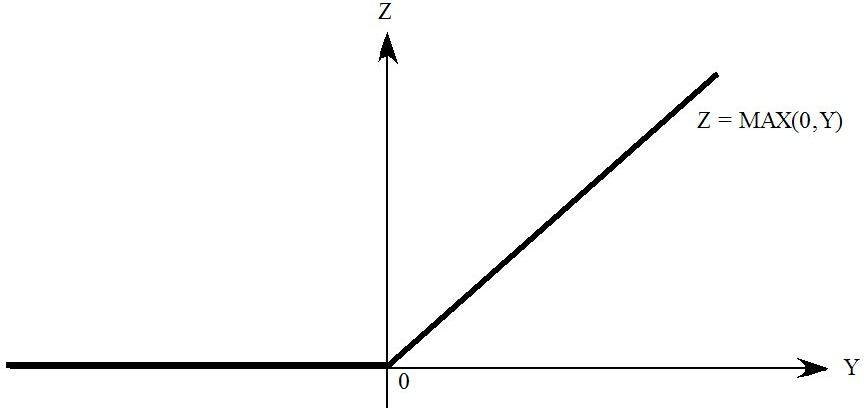
Figure 51.10 Z = MIN(0,Y)
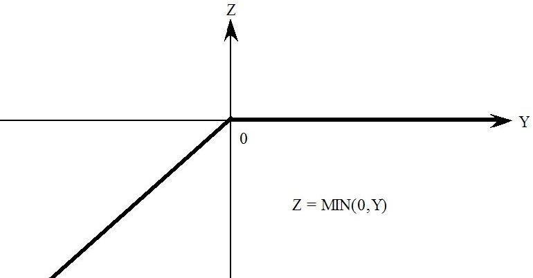
Z = MIN(X,Y)
| Firstly note that | Z = MIN(X,Y) |
| is the same as | Z - X = MIN(0,Y - X). |
Thus Z = MIN(X,Y) can be expressed via the statements
VARIABLE (LEVELS) W # Difference between Z and X # ; EQUATION (LEVELS) E_W W = Z - X ; COMPLEMENTARITY (Variable = W, Upper_Bound = 0) C_Z W - (Y-X) ;
An alternative way of expressing Z=MIN(X,Y) can be found in section 51.9.3 below.
51.9.2 Progressive income tax schedule [gpd3.16.9.2]
Consider a progressive income tax schedule as follows:
- for the first $5000 of income, no tax is paid.
- for any income between $5,001 and $20,000, tax is paid at the rate of 10 cents in the dollar.
- for any income above $20,001, tax is paid at the rate of 20 cents in the dollar.
[See Figure 51.11.]
The formula connecting INCOME and TAX is as follows:
| TAX = 0 | if INCOME <= 5000, |
| TAX = 0.1*(INCOME - 5000) | if 5000 <= INCOME <= 20000, |
| TAX = 0.1*15000 + 0.2*(INCOME - 20000) | if INCOME > 20000. |
You can see that the first two parts of this can be expressed by saying that
TAX = MAX( 0, 0.1*(INCOME - 5000) ) .
Hence, if we introduce a new variable TAX2 via
TAX2 = MAX( 0, 0.1*(INCOME - 5000) ) ,
then you can see that the full rule above connecting INCOME and TAX can be expressed via
TAX = MAX( TAX2, 0.1*15000 + 0.2*(INCOME - 20000) ) .
Thus (using sections 51.9.1 and 51.9.1 above) the piecewise linear connection between INCOME and TAX can be expressed in TABLO language as follows21.
VARIABLE (LEVELS) TAX2 # First 2 parts of tax schedule # ;
COMPLEMENTARITY (Variable = TAX2, Lower_Bound = 0) C_TAX2
TAX2 - 0.1*(INCOME - 5000) ;
VARIABLE (LEVELS) TAX3 # Difference between TAX and TAX2 # ;
EQUATION (LEVELS) E_TAX3 TAX3 = TAX - TAX2 ;
COMPLEMENTARITY (Variable = TAX3, Lower_Bound = 0) C_TAX
TAX3 - { [0.1*15000 + 0.2*(INCOME - 20000)] - TAX2 } ;
Figure 51.11 Progressive income tax schedule
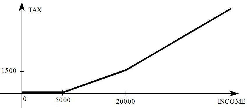
51.9.3 Other piecewise linear functions [gpd3.16.9.3]
You can see from the tax schedule example above that any piecewise linear function can be expressed using various auxiliary variables and Complementarity statements. We give some more examples below.
Z = ABS(X)
Here ABS is for the Absolute Value function — see Figure 51.12.
Since ABS(X) = MAX(X, -X), it is a simple matter to use the details in section 51.9.1 above to express Z = ABS(X) in TABLO language as follows:
VARIABLE (LEVELS) W ; EQUATION (LEVELS) E_W W = Z - X ; COMPLEMENTARITY (Variable = W, Lower_Bound = 0) C_Z W + (2*X) ;
MIN(X,Y) = 0
This relation between X and Y [see Figure 51.10] can be expressed via the statement
COMPLEMENTARITY (Variable = X, Lower_Bound = 0) Comp1 Y ;
Z = MIN(X,Y) Revisited
| If | Z = MIN(X,Y) |
| then | 0 = MIN(X - Z, Y - Z) . |
Hence section 51.9.3 above suggests an alternative to that in section 51.9.1 for expressing Z = MIN(X,Y), namely:
VARIABLE (LEVELS) U # Difference between X and Z # ; EQUATION (LEVELS) E_U U = X - Z ; COMPLEMENTARITY (Variable = U, Lower_Bound = 0) C_MIN Y - Z ;
Figure 51.12 Z = ABS(X)
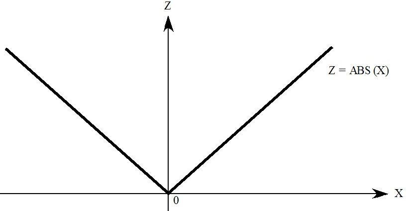
Figure 51.13 MIN(X,Y)=0
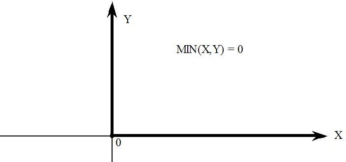
MAX(X,Y) = 0
This relation between X and Y [see Figure 51.14] can be expressed via the statement
COMPLEMENTARITY (Variable = X, Upper_Bound = 0) Comp2 Y ;
Z = MAX(X,Y) Revisited
| If | Z = MAX(X,Y) |
| then | 0 = MAX(X - Z, Y - Z) . |
Hence section 51.9.3 above suggests an alternative to that in section 51.9.1 for expressing Z = MAX(X,Y), namely:
VARIABLE (LEVELS) U # Difference between X and Z # ; EQUATION (LEVELS) E_U U = X - Z ; COMPLEMENTARITY (Variable = U, Lower_Bound = 0) C_MAX Y - Z ;
Figure 51.14 MAX(X,Y) = 0
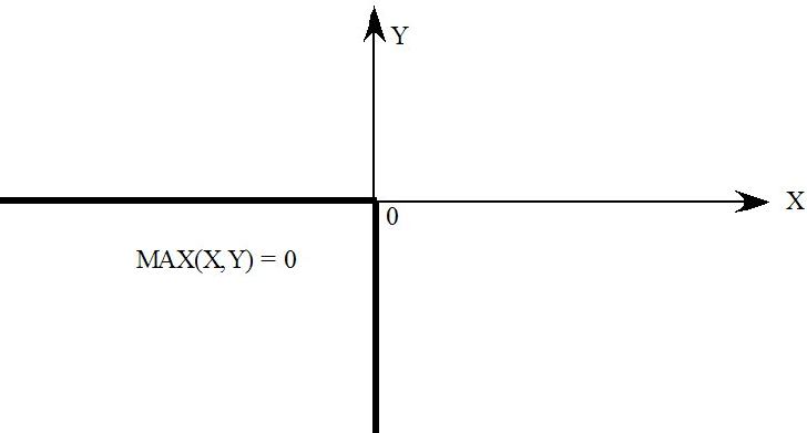
51.10 Example: ORANIGRD (ensuring investment stays non-negative) [gpd3.16.10]
In many models, investment is determined endogenously as a function of rates of return. If the rate of return in an industry increases, this is a signal to increase investment in that industry, while if the rate of return falls, investment falls. In the latter case, care must be taken to ensure that the functional relationship between investment and the rate of return does not result in negative investment.
In this example,
- we show how negative investment can occur in a simple modification of the ORANIGRD model.
- we show how to modify the functional relationship between investment and the rate of return using a Complementarity to ensure that investment is always non-negative.
ORANIGRD (see section 60.14) is a recursive dynamic version of the well-known ORANIG model. [The "RD" at the end of ORANIGRD stands for "recursive dynamic".] The ORANIGRD model was built by Mark Horridge.
In ORANIGRD,
- GROSSRET stands for the GROSS rate of RETurn in an industry - this is equal to capital rentals divided by the value of the capital stock.
- GROSSGRO stands for the GROSS GROwth rate in investment - this is equal to the value of investment divided by the value of the capital stock.
The files for the examples described here can be found in zip file ORANIGRD.ZIP supplied with GEMPACK.
51.10.1 OGRD1.TAB and negative investment [gpd3.16.10.1]
ORANIGRD.TAB contains several alternative ways of determining investment22.
In OGRD1.TAB we have added an alternative way of determining investment (added to the bottom of the TAB file). This modified way of determining investment is the simple rule
delGGRO = alpha * delGRET (INV5A)
where delGGRO is a linear variable equal to the change in GROSSGRO and delGRET is a linear variable equal to the change in GROSSRET. The simple investment rule INV5A above says that the change in GROSSGRO is alpha times the change in GROSSRET (where alpha is a parameter which is set equal to 3 in OGRD1.TAB).
The problem with this (and other similar) investment rules is that, if GROSSRET falls sufficiently, the resulting negative change in GROSSRET may result in negative GROSSRET and hence in negative investment.
You can see this if you run the simulation in OGRD1.CMF in which a uniform negative technological progress is applied to all primary factors23. [The variable a1prim is shocked by 2 which indicates technical regress.] Investment in industry "OthMining" [Other Mining] falls by 108 percent, which means that investment has become negative. [To see this, look at the results for variable x2tot which is the percentage change in investment by industry.]
51.10.2 OGRD2.TAB - A complementarity to ensure non-negative investment [gpd3.16.10.2]
In the levels, the simple rule INV5A above corresponds to a linear (straight line) relationship between GROSSGORO and GORSSRET as shown in Figure 51.15. This will result in negative GROSSGRO and hence negative investment if GROSSRET falls below the value indicated by point N in that figure.
The levels form of the equation is
GROSSGRO = alpha*GROSSRET + FINV5
where FINV5 is the value of the Y-intercept (that is, the value of GROSSGRO when GROSSRET=0)24.
The obvious way to modify the simple investment rule INV5A above is to use it as long as it keeps investment positive but then to override it if it would imply negative investment. For example, use INV5A if it results in positive investment, otherwise set investment equal to zero. This would result in GROSSGRO being determined by the function shown in Figure 51.16. The function there has the equation
GROSSGRO = MAX( alpha*GROSSRET + FINV5 , 0) . (INV5B)
Alternatively, you may prefer to always leave a small positive investment in each industry. This is what we have done in OGRD2.TAB in which the relationship between GROSSGRO and GROSSRET is
GROSSGRO = MAX( alpha*GROSSRET + FINV5 , GGRO_LBOUND) . (INV5C)
where GGRO_LBOUND is a lower bound on the possible values for GROSSGRO. We have set GGRO_LBOUND equal to one-tenth of the initial (that is, pre-simulation) value of GROSSGRO in each industry. See Figure 51.17.
This modified investment rule INV5C is a piecewise linear function involving MAX. As we have seen above (section 51.9.1), this can be represented accurately via a Complementarity statement. This is done in OGRD2.TAB where the Complementarity statement is25.
Complementarity (Variable = GROSSGRO_L, Lower_Bound = GGRO_LBOUND) C_FINV5 # Simple investment rule - complementarity version # (all,i,IND) GROSSGRO_L(i) - [GGRO_GRET(i)*GROSSRET_L(i) + FINV5_L(i)] ;
You can see that this keeps investment non-negative if you run the simulation in OGRD2.CMF in which the same uniform negative technological progress is applied to all primary factors as in OGRD1.CMF26. Investment in industry "OthMining" [Other Mining] now falls by just 90 percent (since GROSSGRO is not allowed to fall below the lower bound equal to 10% of its original value and since capital stock does not change in this simulation). [To see this, look at the results for variable x2tot which is the percentage change in investment by industry.]
Of course there are several other investment rules which ensure that investment does not become negative. Many would involve MAX (as did our example above).27.
Figure 51.15 Linear investment rule INVA
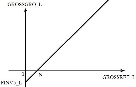
Figure 51.16 Non-negative investment rule INVB

Figure 51.17 Non-negative investment rule INVC
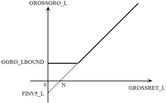
51.11 Complementarities - speeding up single Euler calculations [gpd9.7.18]
Explanation
It is traditional to solve some large models, including the MMRF and TERM models used at the Centre of Policy Studies, using a single multi-step Euler calculation - for example, an Euler 8-step28.
When there are Complementarity statements in the model, the CPU time (see section 49.2) is roughly doubled compared to the same model with these Complementarity statements omitted. The doubling comes from the need to do the approximate run and then the accurate run.
When extrapolation is used, the accurate run usually produces a much more accurate solution than the approximate run. We strongly recommend that you do the accurate run when you would normally extrapolate from 2 or 3 multi-step calculations when solving your model.
But when the accurate run is done via a single Euler multi-step calculation, the accurate run results are probably hardly (if at all) more accurate than those from the approximate run - this is explained in section 51.11.1 below. In that case, it may make sense to omit the accurate run, since that will reduce the total CPU time by about 50%. The accurate run will be omitted if you include the statement
complementarity do_acc_run = no ;
in your Command file (see section 51.5.6).
There are some restrictions as noted in section 51.5.6, namely the solution method must be a single multi-step Euler, and only one subinterval is allowed and automatic accuracy is not allowed.
51.11.1 Accuracy of approximate and accurate runs using Euler [gpd9.7.18.1]
This compares the accuracy of the approximate and accurate runs when the accurate run is done using a single Euler multi-step calculation (eg Euler 8-step).
Recall that, during the approximate run, a step is normally29 redone if there is a state change. The step is redone with a shorter step length so that the state change occurs just before the end of the step. This ensures that the simulation does not overshoot a bound by very much. See section 51.7.3 for details.
This redoing of steps, coupled with the Newton correction terms (see, for example, Figure 51.4), means that the approximate run should be nearly as accurate as the following accurate run if you are using just a single Euler multi-step calculation for the accurate run. But it may still result in small overshooting of bounds which should not happen during the accurate run.
Example
Consider an import quota simulation such as in Figures 51.1 to 51.4. There may be small overshooting of the quota bound on the approximate run (despite redoing steps and despite the Newton correction terms). But there should be no overshooting on the accurate run since then the closure is changed and a shock to the import volume is given so that it exactly hits the quota bound.
You may decide that the slight overshooting from the approximate run may be acceptable in order to gain the speed increase from not doing the accurate run.
52 Subtotals with complementarity statements [gpd5.7]
Click here for detailed chapter contents
Subtotals in models with complementarities need careful handling, as we learned some time after subtotals were introduced in Release 8.0 (October 2002). Users passed on applications in which there were bugs or the subtotals results calculated on the accurate run were not as expected. These examples were an important catalyst for the new features in Release 9 for subtotals results from models with complementarities. We describe these new features below.
In running a model containing complementarity statements, two runs are carried out. First an approximate simulation using a single Euler many-step calculation is run to see what state each complementarity is at the end of the run. Secondly an accurate run is carried out after a closure swap. The purpose of these two runs is described in chapter 51.
Subtotals and the Accurate Run
Subtotals calculated during the accurate complementarity run are not easy to interpret. We do not recommend that you calculate or report them. [See section 52.3 below for more details.]
Subtotals and the Approximate Run
We recommend that you calculate and report subtotals calculated during the approximate complementarity run because they are easy to interpret and give you what you expect. See section 52.2 below for more details.
Decomposition of Results
By "decomposition", we mean that you set up subtotals where each shock applied in the simulation is in just one subtotal. The sum of the subtotals should add up to exactly the total cumulative solution.
Details about how to use subtotals to decompose your results during the approximate run are given in section 52.2. We recommend that you use this method. Details about decomposing results during the accurate run are give in section 52.3 below but we do not recommend that you use subtotals during the accurate run when reporting your work because the subtotals are difficult to interpret and are not robust.
The main points about decomposition are:
- To complete a decomposition on the approximate run, you need to include the Newton correction variable $del_Comp (see section 51.7.2) in one of the subtotals (preferably its own). If this variable is the only shocked variable in a subtotal, that subtotal can be interpreted as the consequences of overshooting the complementarity bounds on Euler steps. [See section 52.2 below for more details.]
- To complete a decomposition on the accurate run, you need to include in subtotals some variables introduced by the software (see section 51.7.2).
We elaborate on these points below.
52.1 Telling the software when to calculate subtotals [gpd5.7.1]
There are Command file statements that apply when you are solving a model containing Complementarity statements.
You can tell the software whether to calculate subtotals on the approximate run (recommended) or on the accurate run (not recommended) via the following Command file statement.
complementarity subtotals = APPROXIMATE|accurate ; ! default is "approximate"
This tells if subtotals are to be calculated during the approximate run or during the accurate run.
The default is APPROXIMATE unless the simulation is only doing the accurate run.
You can include the results of the approximate run as a subtotal on the Solution file via the following Command file statement.
complementarity approx_as_subtot = first|last|yes|no ;
This tells if the cumulative solution from the approximate run will be added as a subtotal solution.
- first or yes means that it will be added as the first subtotal (before any subtotals defined by "subtotal" statements in the Command file),
- last means that it will be added as the last subtotal (after any subtotals defined by "subtotal" statements in the Command file),
- no means that it will not be added as a subtotal.
If there are any subtotal statements in your Command file and you are calculating these subtotals on the approximate run, the default is first. Otherwise the default is no.
Example:
Run TABLO with the TAB file MOIQ.TAB and then run a simulation using the Command file MOIQ3.CMF supplied with the Examples files1. Notice that MOIQ3.CMF does not contain either of the two statements above, so the default values apply. This is equivalent to having the following statements in the Command file:
complementarity subtotals = approximate; complementarity approx_as_subtot = first ;
There are four subtotal statements in MOIQ3.CMF:
subtotal p_XImp_Quota = XImp_quota changes ; subtotal p_TIMP = TIMP changes ; subtotal $del_comp = complementarity overshooting ; subtotal p_XImp_Quota $del_comp p_TIMP = ALL changes ;
If you look at MOIQ3.SL4 in ViewSOL, it has 5 subtotal columns but the first "subtotal" is the cumulative solution from the approximate run. Click on the ViewSOL Menu item Description to see that the subtotals are:
- Cumulative solution from the approximate run
- XImp_quota changes
- TIMP changes
- complementarity overshooting
- ALL changes
Notice also that, as expected, results in the first subtotal (cumulative solution from the approximate run) differ slightly from the cumulative solution for the accurate run (which is the true solution of the simulation).
Subtotal results 2, 3 and 4 above are a decomposition of the solution from the approximate run. Thus they add to the solution from the approximate run but do not add exactly to the solution from the accurate run. We say more about this in section 52.2.1 below.
52.2 Calculating subtotals on the approximate run - recommended [gpd5.7.2]
We believe that the natural time to calculate subtotals is on the approximate run. You are then calculating what you expect based on the closure and shocks in the Command file for the simulation. However, if you calculate subtotals on the accurate run (when the software may modify the closure and shocks2), we are not sure how to interpret the results — see section 52.3 below.
If you specify subtotals whose related exogenous variables cover all the shocked variables (including the Newton correction variable $del_Comp — see section 51.7.2), the relevant subtotal results add exactly to the cumulative solution from the approximate run. That is, it is relatively easy to decompose the approximate result into several natural subtotals (provided you remember to include the Newton correction variable $del_Comp in one subtotal).
In tests we have carried out, the subtotal results are robust to variations in the number of subintervals. [That is, you get similar subtotal results for the same simulation with one, two or several subintervals.]
52.2.1 Decomposed results do not sum to accurate cumulative solution [gpd5.7.2.1]
Unfortunately there is a downside to this. The cumulative solution from the approximate run will usually be slightly different from the cumulative solution from the accurate run. And it is the latter (the cumulative solution from the accurate run) which you will want to report as the results of your application. So, if your subtotals cover all the shocks,
- the good news is that the subtotals results from the approximate run are an exact decomposition of the cumulative solution from the approximate run (and these subtotals results are what you expect from subtotals results), but
- the bad news is that these subtotals results are not an exact decomposition of the cumulative solution you wish to report, namely the cumulative solution from the accurate run.
You noticed these points when you carried out the MOIQ3.CMF simulation in section 52.1 above. We discuss this and related simulations in more detail in section 52.4 below.
If you are not reporting a decomposition, but just some interesting subtotals, there is no problem.
If you are reporting a decomposition, you might note (perhaps in a footnote) that the decomposition results only add approximately to the results reported. Or you might like to scale the subtotals results so that they do add exactly. [If so, you will need to scale them differently for each endogenous result you report.]
We will be interested to hear from users as to how they decide to handle this dilemma.
Note that this problem is not a really serious one since subtotals results are only a rough attribution of the contribution of a group of shocks within the context of a simulation. See chapter 29 and HHP) for more details. For example, the subtotals results depend on the path of the simulation (see section 29.6).] In particular, you should never regard subtotals results as definitively as you regard the accurate cumulative solution from a simulation.
52.3 Calculating subtotals on the accurate run - not recommended [gpd5.7.3]
In order to calculate on the accurate run subtotals which add to the cumulative result, you need to include in subtotals some variables added by the system for complementarities.
We do not recommend reporting subtotals results calculated during the accurate run.
- We do not know how to interpret the subtotal results reported from some standard simulations.
- The results are not robust since the results calculated change significantly as the number of subintervals changes.
The results in section 52.4.4 illustrate these points.
Notice that the closure on the accurate run may change from subinterval to subinterval. This is because the target states can vary on each subinterval. [For example, there may be no state changes during subinterval 1 but one or more state changes during the second subinterval.]
For these reasons, if you calculate subtotals on the accurate run, you will see that the shocked components included in each subtotal are re-examined at the start of the accurate run in each subinterval.
52.3.1 Decomposing accurate - include extra variables in subtotals [gpd5.7.3.1]
If, despite our recommendation in section 52.3 above, you want to produce subtotals results which decompose the accurate simulation result, you need to explicitly include the relevant extra variables (as documented in section 51.7.2) in subtotals statements. These variables are
- the complementarity expression variable (whose name ends with "@E") - for example, c_IMPQUOTA@E in the MOIQ3 example below,
- the complementarity variable (p_TIMP_QUOTA in the MOIQ3 example below).
[You never need to include the lower bound or upper bound variables (their names end with "@L" or "@U" — see section 51.7.2) since they are always endogenous (if they are needed).3 ]
Note also that you can use levels names rather than the associated linear variables. For example, the four subtotals statements we have included in MOIQ3AC.CMF:
subtotal XImp_Quota = XImp_Quota changes ; subtotal IMPQUOTA@E TIMP_QUOTA = IMPQUOTA state changes ; subtotal TIMP = TIMP changes ; subtotal XImp_Quota IMPQUOTA@E TIMP_QUOTA TIMP = ALL changes ;
all use levels names.
In general, for each complementarity we recommend that you include a separate subtotal statement which reports the consequences of any state changes in that complementarity.
For example, suppose you have a Complementarity called COMP1 in the TAB file and that the associated complementarity levels variable is called LEV_COMP1. Then you could include the subtotal statement
subtotal LEV_COMP1 COMP1@E = COMP1 state changes ;
to capture the consequences of any state changes in that complementarity. [You would probably want to include such a subtotal statement for every complementarity in the model.]
In the example MOIQ3AC.CMF, the subtotal is called IMPQUOTA and the associated complementarity variable is TIMP_QUOTA, so the subtotal statement is (using levels names)
subtotal IMPQUOTA@E TIMP_QUOTA = IMPQUOTA state changes ;
or, using linear variable names,
subtotal c_IMPQUOTA@E p_TIMP_QUOTA = IMPQUOTA state changes ;
See the MOIQ3AC.CMF examples given in section 52.4.1 below.
52.4 Examples: MOIQ3.CMF and related simulations [gpd5.7.4]
In Release 8.0 of GEMPACK, the examples subdirectory contains the TABLO Input file for the MOIQ model, MOIQ.TAB, and also the Command file MOIQ1C.CMF which runs a simulation to decrease the import quota volume of commodity 1 by 30%. This decrease makes the import quota binding for commodity 1. The shock in the Command file MOIQ1C.CMF is
shock p_XImp_Quota = -30 0 ;
Below we use a simulation in MOIQ3.CMF that is similar to the Command file MOIQ1C.CMF distributed with Release 8.0 of GEMPACK4.
The difference between the original simulation in MOIQ1C.CMF and the simulation in MOIQ3.CMF is that an additional shock has been added. The additional shock statement in MOIQ3.CMF is:
shock p_TIMP = uniform 5 ;
This extra shock is added in this example so that we have more shocks to use in examples of subtotal statements. The closure and shocks in MOIQ3.CMF are shown below.
Closure and shocks in MOIQ3.CMF
exogenous p_PIMP p_FEXP p_XEXP("c2") p_PHI
p_V 1 p_FWAGE p_CR p_TIMP p_XCAP
p_XImp_Quota
;
rest endogenous ;
shock p_XImp_Quota = -30 0 ;
shock p_TIMP = uniform 5 ;
In MOIQ1C.CMF and in MOIQ3.CMF, there are 20 Euler steps on the approximate run.
complementarity steps_approx_run = 20 ;
The subtotals statements in MOIQ3.CMF are shown below.
Subtotal statements in command file MOIQ3.CMF
! Subtotals - decompose cumulative result from approximate run subtotal p_XImp_Quota = XImp_quota changes ; subtotal p_TIMP = TIMP changes ; subtotal $del_comp = complementarity overshooting ; subtotal p_XImp_Quota $del_comp p_TIMP = ALL changes ;.
As discussed in section 52.2 above, in order to get a decomposition on the approximate run, you need to include the Newton-correction complementarity variable $del_Comp in one subtotal. The variable $del_Comp is used during the approximate run to generate Newton correction terms that force the solution path back onto the appropriate branch of the complementarity condition if the step has overshot. This is discussed in section 51.7.2 and in section 11.14.
You must not add $del_Comp to the list of exogenous variables, or to the list of shocks, in your Command file - it is automatically exogenous and given a shock of 1 in the approximate run (see section 51.7.2). However you do need to add it to one of the subtotals if you are trying to decompose the cumulative results from the approximate run (which is what we recommend for decompositions). You can see that $del_Comp is in the third subtotal above. You will see later, when we discuss the results, why we give the description "complementarity overshooting" to this subtotal.
The simulation MOIQ3.CMF decomposes the cumulative results for the approximate run into three subtotals (the first three above) whose results add to the cumulative result. [The results of the fourth subtotal "ALL changes" above should equal the cumulative result from the approximate run since all shocked variables are in that subtotal.]
The full MOIQ3.CMF Command file is shown on in Figure 52.1.
We have also supplied some variants of MOIQ3.CMF to illustrate various points. These variants, whose names begin with MOIQ3 (for example, MOIQ3AC.CMF and MOIQ32I.CMF), are discussed below. The variants have the same closure and shocks as in MOIQ3.CMF but have different Command file statements to say when subtotals are calculated and to vary the number of subintervals.
Figure 52.1 Command file MOIQ3.CMF
! GEMPACK Command file for running
! GEMSIM or the TABLO-generated program
! for the Mixed Levels/Linear version (MOIQ.TAB)
! of the Miniature ORANI model (not condensed) with Import Quotas
! Steps in approximate run
complementarity steps_approx_run = 20 ;
! Solution method and steps
method = gragg ;
steps = 6 8 10 ;
verbal description =
Quota test.
Illustrate decomposition of results from approximate run ;
! Auxiliary files
auxiliary files = moiq ;
! Input data
file basedata = mo.dat ;
file quota_ratios = moiq_rat.dat ;
! Updated data
updated file basedata = <cmf>.upd ;
updated file quota_ratios = <cmf>q.upd ;
extrapolation accuracy file = yes ;
log file = yes ;
! Closure
exogenous p_PIMP p_FEXP p_XEXP("c2") p_PHI
p_V 1 p_FWAGE p_CR p_TIMP p_XCAP
p_XImp_Quota ;
rest endogenous ;
! Shocks
shock p_XImp_Quota = -30 0 ;
shock p_TIMP = uniform 5 ;
! Subtotals - decompose cumulative result from approximate run
subtotal p_XImp_Quota = XImp_quota changes ;
subtotal p_TIMP = TIMP changes ;
subtotal $del_comp = complementarity overshooting ;
subtotal p_XImp_Quota $del_comp p_TIMP = ALL changes ;
52.4.1 Example: MOIQ3AC.CMF simulation [gpd5.7.4.1]
Before we discuss the results of the MOIQ3.CMF simulation, we describe a similar Command file MOIQ3AC.CMF. This carries out the same simulation but calculates subtotals which decomposes the cumulative result from the accurate simulation (rather than the approximate one as in MOIQ3.CMF).
The relevant statements in MOIQ3AC.CMF are shown below.
Subtotal statements in command file MOIQ3AC.CMF
! Subtotals for accurate run (not recommended)
! Next tells program to calculate subtotals on accurate run.
! [The default is to calculate subtotals on the approximate run.]
complementarity subtotals = accurate ;
! Subtotals - decompose cumulative result from accurate run
subtotal p_XImp_Quota = XImp_quota changes ;
subtotal p_TIMP = TIMP changes ;
subtotal IMPQUOTA@E TIMP_QUOTA = IMPQUOTA state changes ;
subtotal XImp_Quota
IMPQUOTA@E TIMP_QUOTA
p_TIMP = ALL changes ;
The versions of GEMSIM and TABLO-generated programs for Release 8.0-001 (October 2003) and later allow you to include the complementarity variables (such as p_IMPQUOTA@E above) in subtotal statements.
The variables listed in the exogenous statement in MOIQ3.CMF are exogenous during both the approximate and the accurate runs5.
Also relevant to the exogenous variables for the accurate run are the complementarity variable and the complementarity expression variable (see section 51.7.2). If the complementarity is in state 1 or 3 after the approximate run, the complementarity variable (p_TIMP_QUOTA in the MOIQ model) is exogenous and shocked in the accurate run. If the complementarity is in state 2 after the approximate run, the complementarity expression variable (c_IMPQUOTA@E in the MOIQ model) is exogenous and shocked in the accurate run.
To include the effect of all shocks in the accurate run, you need the third subtotal above
subtotal c_IMPQUOTA@E p_TIMP_QUOTA = IMPQUOTA state changes ;
The description (IMPQUOTA state changes) suggests that you might interpret the results of this subtotal as showing the effects of state changes. You will learn more about that when we discuss the results in section 52.4.4 below.
52.4.2 Several subintervals [gpd5.7.4.2]
When discussing the results, it is useful to also have results from this simulation solved over several subintervals (see section 26.3). We have supplied the following Command files.
- MOIQ3.CMF - the basic simulation (see section 52.4). The subtotals here decompose the cumulative results from the approximate run. Just one subinterval.
- MOIQ3AC.CMF - the same simulation but subtotals decompose the cumulative result from the accurate run (see section 52.4.1). Just one subinterval.
- MOIQ32I.CMF and MOIQ39I.CMF - same as MOIQ3.CMF except these are run over 2 and 9 subintervals respectively.
- MOIQ3AC2.CMF - same as MOIQ3AC.CMF except there are 2 subintervals.
If you have access to Release 9 of GEMPACK, we suggest that you run these 5 simulations now so that you can look at the results as you read our discussion of the results in section 52.4.3 below.
52.4.3 MOIQ3.CMF subtotals calculated during approximate run [gpd5.7.4.3]
In the following sections we will look just at one variable p_CHOUS but the other variables behave in a similar way. You will find the variable p_CHOUS under the heading Macros in ViewSOL.
In MOIQ3.SL4 produced by MOIQ3.CMF, the p_CHOUS result reported (this is from the accurate version of the simulation in each case) is 10.755.
| p_CHOUS = 10.755 | (accurate simulation result from MOIQ3.CMF) |
In MOIQ3.SL4 you can also see the cumulative result for p_CHOUS from the approximate run since the first subtotal results are the cumulative solution from the approximate run. [This is explained in section 52.1 above since the default is "complementarity approx_as_subtot = first ;".] To check this, after you have loaded the MOIQ3 results into ViewSOL make sure that you have selected the moiq3 solution (in the "Choose which solution to view" drop-down box), and then click on Description in the main menu. You will see the descriptions for the different subtotals. Although there are only 4 subtotal statements in MOIQ3.CMF, the software has added the cumulative solution from the approximate run as an extra one and made it the first subtotal. Note that the second subtotal result shown from MOIQ3 shows the effects of the Ximp_Quota changes, the third shows the effects of the TIMP shocks, the fourth show the effects of the $del_Comp shock and the fifth shows the effects of all shocks. Of course the fifth subtotal results are identical to the first subtotal results.]
The p_CHOUS results from MOIQ3.CMF are:
Table 52.1 Subtotals during MOIQ3.CMF approximate run
| p_CHOUS = | |
| 10.755 | (accurate cumulative result) |
| 10.403 | (subtotal 1 - cumulative results from approximate run) |
| 6.435 | (subtotal 2 - XImp_Quota changes ) |
| 3.967 | (subtotal 3 - TImp changes ) |
| 0.0001 | (subtotal 4 - complementarity overshooting ) |
| 10.403 | (subtotal 5 - ALL changes - same as subtotal 1) |
Note that overshooting occurs since the complementarity for commodity C1 changes state after about 10% of the 15th Euler step of 20. But the $del_Comp overshooting subtotal result is very small (about 0.00001) since the software redoes that step to minimise overshooting6.
It is also interesting to note the p_CHOUS result for the accurate version of this simulation, which is 10.755, is not a lot different from the approximate result of 10.403.
As indicated at the beginning of this chapter, we believe that these subtotals results, calculated during the approximate run, are the natural ones to calculate and report.
As we indicated in section 52.2.1 above, there is a downside to reporting subtotals results from the approximate simulation. Even when (as is the case here) the subtotals are a decomposition of all the shocks, they do not add exactly to the cumulative result from the accurate run (though they do add exactly to the cumulative result from the approximate run). Since the p_CHOUS results (and those for other variables) are not much different between the accurate and approximate runs, this is not much of a problem.
You might also like to look at the p_CHOUS results from the Command files MOIQ32I.CMF and MOIQ39I.CMF where 2 and 9 subintervals have been used. The results from MOIQ32I.CMF are
Table 52.2 Subtotals during MOIQ32I.CMF approximate run (2 subintervals)
| p_CHOUS = | |
| 10.755 | (accurate cumulative result) |
| 10.650 | (subtotal 1 - cumulative results from approximate run) |
| 6.684 | (subtotal 2 - XImp_Quota changes ) |
| 3.966 | (subtotal 3 - TImp changes ) |
| 0.0001 | (subtotal 4 - complementarity overshooting ) |
| 10.650 | (subtotal 5 - ALL changes - same as subtotal 1) |
while the results from MOIQ39I.CMF are
Table 52.3 Subtotals during MOIQ39I.CMF approximate run (9 subintervals)
| p_CHOUS = | |
| 10.755 | (accurate cumulative result) |
| 10.739 | (subtotal 1 - cumulative results from approximate run) |
| 6.770 | (subtotal 2 - XImp_Quota changes ) |
| 3.969 | (subtotal 3 - TImp changes ) |
| 0.0001 | (subtotal 4 - complementarity overshooting ) |
| 10.739 | (subtotal 5 - ALL changes - same as subtotal 1) |
Notice that, as expected, the cumulative solution from the approximate run gets closer to the cumulative result from the accurate run when more subintervals are used.
Notice also that the subtotal results don't change by very much. This is in contrast to the subtotal results calculated during the accurate run which (as you will see in section 52.4.4 below) change dramatically if the number of subintervals is changed.
Note that there is only one variable $del_Comp introduced by the software, even if you have several complementarity statements in your model. The subtotal relating to this variable (subtotal 4 in the example above) captures overshooting for all complementarities. There are not separate $del_Comp variables which allow you to separate the effects of overshooting on different Complementarities.
52.4.4 MOIQ3AC.CMF subtotals calculated during accurate run (not recommended) [gpd5.7.4.4]
In MOIQ3AC.SL4 produced by MOIQ3AC.CMF, the p_CHOUS result reported (this is from the accurate version of the simulation in each case) is 10.755.
| 10.755 | (p_CHOUS accurate simulation result from MOIQ3AC.CMF) |
Of course, this is the same as the accurate simulation result from MOIQ3.CMF (see section 52.4.3 above).
The subtotals results in MOIQ3AC.SL4 are
- Ximp_Quota changes (effects of shocks to p_Ximp_Quota). This is subtotal number 1.
- TIMP changes (effects of shocks to p_TIMP). This is subtotal number 2.
- IMPQUOTA state changes (effects of system-supplied shocks to IMPQUOTA@E and TIMP_QUOTA). This is subtotal number 3.
- effect of all shocks. This is subtotal number 4.
Notice that the cumulative solution from the approximate run is not added automatically as a subtotal — see section 52.1 - since the default is "complementarity approx_as_subtot = no ;" when subtotals are calculated during the accurate run.
The p_CHOUS results from MOIQ3AC.CMF are
Table 52.4 Subtotals during MOIQ3AC.CMF accurate run (not recommended)
| p_CHOUS = | |
| 10.755 | (accurate cumulative result) |
| 19.191 | (subtotal 1 - XImp_Quota changes ) |
| 3.485 | (subtotal 2 - TImp changes ) |
| -11.920 | (subtotal 3 - effect of state changes) |
| 10.755 | (subtotal 4 - ALL changes - same as cumulative result) |
Notice that the result for subtotal 1 (Ximp_Quota changes) is dramatically different from MOIQ3.CMF which calculates the subtotals on the approximate run. However the subtotal 2 results (TImp changes) are not so different.
We cannot find any natural interpretation for the first and third subtotals above (the Ximp_Quota changes and the IMPQUOTA state changes results). Since these results are not numerically robust (see just below) perhaps this is not surprising. Subtotals usually depend heavily on the closure and the path so that it is very difficult to interpret the results if the closure and path are changed through the simulation, as happens in the accurate run.
The p_CHOUS results from MOIQ3AC2.CMF (same as MOIQ3AC.CMF except use 2 subintervals) are
Table 52.5 Subtotals during MOIQ3AC2.CMF accurate run 2 subintervals (not recommended)
| p_CHOUS = | |
| 10.755 | (accurate cumulative result) |
| 10.656 | (subtotal 1 - XImp_Quota changes ) |
| 3.841 | (subtotal 2 - TImp changes ) |
| -3.742 | (subtotal 3 - effect of state changes) |
| 10.755 | (subtotal 4 - ALL changes - same as cumulative result) |
Notice that the results for subtotals 1 and 3 are dramatically different from those from MOIQ3AC.CMF when only one subinterval is used. This is a clear illustration as to why we do not recommend calculating subtotals during the accurate run.
- Subtotals results calculated during the accurate run are not robust. [For example, they can change a lot if the number of subintervals is changed.]
- Hence we do not know how to interpret subtotals results when calculated during the accurate run.
We elaborate on this in section 52.4.5 below.
Fortunately, these problems do not occur when subtotals are calculated during the approximate run.
52.4.5 Subtotals from accurate run not robust [gpd5.7.4.5]
The subtotals results from the accurate run change dramatically if several subintervals are used. We report some of these results (based on MOIQ3AC.CMF with one or more subintervals) below.
We think we understand why these results are not robust and include our reasons later in this section.
The results below come from calculating subtotals in MOIQ3AC.CMF on the accurate run.
- Subtotal 1 refers to the XImp_Quota changes,
- Subtotal 2 refers to the TIMP changes, and
- Subtotal 3 refers to the IMPQUOTA state changes.
The p_CHOUS results from MOIQ3AC.CMF are over 1 subinterval (for 6 8 10 Gragg)
| 10.755 (sim) | 19.191 (subtot 1) | 3.485 (subtot 2) | -11.920 (subtot 3) |
Now, suppose that we solve this over 2 subintervals (6 8 10 Gragg) [MOIQ3AC2.CMF]. The p_CHOUS results are
| 10.755 (sim) | 10.657 (subtot 1) | 3.841 (subtot 2) | -3.742 (subtot 3) |
Note that subtotals results 1 and 2 have changed dramatically.
Now, suppose that we solve this over 20 subintervals (6 8 10 Gragg). The p_CHOUS results are
| 10.755 (sim) | 7.668 (subtot 1) | 3.934 (subtot 2) | -0.847 (subtot 3) |
Note that subtotals results 1 and 2 have changed dramatically again.
We think that we understand what is happening, at least in this simulation. We explain this below. This explanation relies on a detailed understanding of the closure swap made during the accurate simulation, and is somewhat complicated. It is not essential that you understand this explanation, so feel free to skip on the next subsection 52.4.6.
In this simulation, there is just one state change. The state of complementarity IMPQUOTA for the first commodity C1 changes from being in state 1 (non-binding quota) to state 2 (binding quota) about three-quarters of the way along the simulation. When we break the simulation up into 20 subintervals, this state change happens in just one of them (actually in subinterval number 14). It is only in this subinterval that the complementarity variables IMPQUOTA@E and TIMP_QUOTA which make up subtotal number 3 receive nonzero shocks. [To understand this, see section 51.7.1.] So subtotal number 3 only has a nonzero value in this single subinterval. And, the size of the subtotal in that single subinterval cannot be too large because only part of the overall shock is being applied there.
Indeed, suppose that we broke up the simulation into just three subintervals of unequal length. Suppose that the first subinterval takes the simulation up until just before this state change. Suppose that the second subinterval is very small and just takes the simulation from where the quota is nearly binding to where it has just become binding. And suppose that the third subinterval completes the simulation. Clearly the subtotal 3 result will be very small since it only has a nonzero value in the tiny subinterval number 2.
This is the intuition behind our understanding of subtotal number 3. If you use a very large number of equal-sized subintervals, the result for subtotal number 3 must be small since it only gets a nonzero value in one of these subintervals. As the number of subintervals increases, this subtotal number 3 must get closer and closer to zero.
To check that, we ran the simulation with 100 subintervals. The results for p_CHOUS are
| 10.755 (sim) | 6.884 (subtot 1) | 3.936 (subtot 2) | -0.094 (subtot 3) |
Sure enough, the subtotal 3 result has become smaller again, as expected.
Notice also that the results for subtotal number 2 (effects of the TIMP shock) are hardly changing as we vary the number of subintervals. This subtotal result is almost the same as the corresponding subtotal calculated during the approximate run. Indeed the subtotals results for p_CHOUS calculated during the approximate run are (see the MOIQ3.CMF results quoted in section 52.4.3 above)
| 10.403 (subtot 1) | 6.435 (subtot 2) | 3.967 (subtot 3) | 0.0001 (subtot 4) |
Here subtotal number 1 is the cumulative solution from the approximate run, subtotal number 2 is the effect of the XIMP_QUOTA shock, subtotal number 3 is the effects of the TIMP shock and subtotal number 4 is the effects of the $del_Comp shock. Thus the effects of the TIMP shock are very similar in the approximate run and in the accurate run, irrespective of the number of subintervals used for the accurate run. And the effects of the XIMP_QUOTA shock are very similar in the approximate run (6.435) and in the accurate run when many subintervals are used (6.884 with 100 subintervals).
This provides another perspective on calculating subtotals on the accurate run. We don't trust them since they are not robust (they change greatly if we change the number of subintervals), as the example above shows. Perhaps they give meaningful results if we were to use a very large number of subintervals since that limits the influence of the shocks to the quota variables (IMPQUOTA@E and TIMP_QUOTA in this model). But there is no point in having to use a large number of subintervals to calculate subtotals in the accurate case. You can more easily calculate subtotals during the approximate run (usually with just one subinterval) and subtotals calculated during the approximate run seem to capture what we expect of subtotals.
This completes our example which shows conclusively that subtotals results on the accurate run are not robust because they may change dramatically if you use more or less subintervals.
52.4.6 Subtotals from approximate run are robust [gpd5.7.4.6]
Contrast the non-robustness of subtotals from the accurate run with subtotals calculated on the approximate run. We have seen in section 52.4.3 above that, when a decomposition of the approximate simulation is calculated using 20 Euler steps on 1, 2 or 9 subintervals, the results hardly change as we vary the number of subintervals.
Below
- Subtotal 1 is the cumulative solution from the approximate run,
- Subtotal 2 refers to the XImp_Quota changes,
- Subtotal 3 refers to the TIMP changes, and
- Subtotal 4 refers to the effects of overshooting ($del_Comp shock).
For 20 Euler steps with 1 subinterval, the p_CHOUS values are:
| 10.370 (subtot 1) | 6.435 (subtot 2) | 3.967 (subtot 3) | 0.00001 (subtot 4) |
For 100 Euler steps with 1 subinterval [MOIQ3A2.CMF], the p_CHOUS values are:
| 10.683 (subtot 1) | 6.715 (subtot 2) | 3.969 (subtot 3) | 0.00002 (subtot 4) |
The cumulative result from this approximate run has moved closer to the accurate result of 10.755. The other subtotal results have not changed significantly.
For 1000 Euler steps with 1 subinterval [MOIQ3A3.CMF], the p_CHOUS values are:
| 10.748 (subtot 1) | 6.779 (subtot 2) | 3.969 (subtot 3) | 0.000002 (subtot 4) |
This further reinforces our recommendation to calculate and report subtotals from the approximate run, rather than from the accurate run.
Subtotals results from the approximate run are robust and relatively easy to interpret.
However,
Subtotals results from the accurate run are not robust and are difficult to interpret.
52.4.7 The initial closure is shown on solution files [gpd5.7.4.7]
Although the cumulative results shown on the Solution file (and hence, in ViewSOL and AnalyseGE) are those from the accurate simulation, the closure stored on the Solution file is the original closure (that is, the closure for the approximate simulation). [Remember that ViewSOL shows results for exogenous variables in red and results for endogenous variables in black.] We think that the closure from the approximate simulation is the natural one for you to see since it is the closure you specified in the Command file.
We apologise for not documenting this in the Release 8.0 documentation.
For example, in the MOIQ3.CMF simulation in section 52.4 above, ViewSOL indicates that both components of the variable p_IMPQUOTA@E are endogenous, even though the C1 component is shocked by -0.2 in the accurate simulation, and is included in the third subtotal in section 52.4.1 above. Similarly ViewSOL shows that the both components of the complementarity dummy variable $IMPQUOTA@D are exogenous even though they are endogenous in the accurate simulation (see section 51.7.2).
52.5 Variables with no components exogenous allowed in subtotals [gpd5.7.5]
In order to allow subtotals which constitute a decomposition to be calculated during the accurate run, we softened [in Release 8.0-001 (October 2003)] the testing of variables that are allowed in a subtotal statement. You are now allowed to include all components of a variable, none of whose components are exogenous. [But you are not allowed to specify just some components of a variable if these components are not exogenous.7 ]
Example: Consider the third subtotal statement in MOIQ3AC.CMF (see section 52.4.1 above).
subtotal IMPQUOTA@E TIMP_QUOTA = IMPQUOTA state changes ;
Here all components of variables IMPQUOTA@E and TIMP_QUOTA are included in this subtotal.
If there are no state changes then, since both quotas are non-binding in the initial data, both components of TIMP_QUOTA will be exogenous (and given shocks of zero) while no components of IMPQUOTA@E will be exogenous. Under the checking rules in force in Release 8.0, that statement would not be allowed. It is now allowed.
53 More examples of post-simulation processing [postsim2]
Click here for detailed chapter contents
In this chapter we give several examples of PostSim processing in a TAB file (see chapter 12). These are all based on Examples files distributed with GEMPACK. We encourage you to work through these examples on your computer as you are reading about them.
We point out in section 53.3 that much of the sophisticated post-simulation processing (such as is currently available with the GTAP model and some other standard models) could more easily now be done using PostSim statements in the main model TAB file. Similar sophisticated post-simulation processing could easily be added to other models.
53.1 Examples — summaries of the updated data [gpd5.2.1]
Many models write summaries of the salient features of a database as part of the TAB file used to solve the model, or in a related TAB file. Below you can work through examples based on ORANIG03.TAB and GTAP61.TAB. The relevant TAB and Command files are in the supplied GEMPACK examples.
53.1.1 Adding some PostSim processing to ORANIG03.TAB [gpd5.2.1.1]
In ORANIG03.TAB1, summary information is written to the logical file SUMMARY using statements such as:
Code in ORANIG03.TAB
Set INCMAC # Income Aggregates # (Land, Labour, Capital, IndirectTax);
Coefficient (all,i,INCMAC) INCGDP(i) # Income Aggregates #;
Formula
INCGDP("Land") = V1LND_I;
INCGDP("Labour") = V1LAB_IO;
INCGDP("Capital") = V1CAP_I;
INCGDP("IndirectTax") = V0TAX_CSI;
Write INCGDP to file SUMMARY header "IMAC";
These statements collect together the aggregates that make up GDP from the income side V1LND_I, V1LAB_IO, V1CAP_I and V0TAX_CSI into one Coefficient INCGDP and write the values to the SUMMARY file. These are calculated from the pre-simulation data on the BASEDATA file.
As an example, the simulation in ORNG03SR.CMF is a 5 percent cut in the real wage using the short-run closure2. The following table shows INCGDP values on the SUMMARY file SUMMARY.HAR produced when you carry out this simulation. The values shown reflect the values in the original data OZDAT934.HAR.
Table 53.1 Initial INCGDP values from original data file
| IMAC | INCGDP |
| Land | 2735.663 |
| Labour | 194981.218 |
| Capital | 180575.218 |
| IndirectTax | 49512.164 |
| Total | 427804.250 |
Using PostSim statements, you can easily arrange for the calculation of summary facts based on the updated data to happen as part of the original simulation. All you have to do is to duplicate the write statements, as shown below.
For example, you could add the following statements:
PostSim code in OG03PS.TAB
File (New) SUMMARY_UPD # Summary info for updated data #; Write (PostSim) INCGDP to file SUMMARY_UPD header "IMAC" ;
We have added these statements to ORANIG03.TAB to produce the new file OG03PS.TAB3.
Because the Write statement above includes the qualifier (PostSim), the values of the GDP aggregates INCGDP written to file Summary_UPD will be the updated or post-simulation values.
We suggest that you carry out the wage-cut simulation using OG03PS.TAB, and following these steps:
(a) first implement OG03PS.TAB by running TABLO taking inputs from the Stored-input file OG03PSGS.STI. This produces output for GEMSIM.
(b) then carry out the simulation using Command file WAGEPS.CMF4. This has the same shock as in ORNG03SR.CMF but it is set up to carry out the simulation accurately (Gragg 2,4,6) based on OG03PS.TAB.
(c) Then look at the two Summary files produced. The first one is the file with logical name SUMMARY. The version of this file produced during the WAGEPS.CMF simulation is called WAGEPS-SUM.HAR since the Command file statement is
file Summary = <cmf>-sum.har ;
This file should contain INCGDP values based on the pre-simulation data as shown in the table above.
(d) The second one is the file with logical name Summary_UPD. The version of this file produced during the WAGEPS.CMF simulation is called WAGEPS-SUM-UPD.HAR since the Command file statement is
file Summary_UPD = <cmf>-sum-upd.har ;
This file contains INCGPD values based on the post-simulation data (since there is a "PostSim" qualifier in the Write statement added to OG03PS.TAB). The values should be as shown below.
Table 53.2 Post-simulation values of INCGDP
| IMAC | INCGDP |
| Land | 2940.36 |
| Labour | 185162.02 |
| Capital | 180363.03 |
| IndirectTax | 49623.88 |
| Total | 418089.28 |
For example, you can see that the value of INCGDP("labour") falls by roughly 5 percent from 194981 in the original data to 185162 in the updated data.
How is the PostSim value of INCGDP("Labour") calculated?
Initially V1LAB values are read in from file BASEDATA. After the simulation, V1LAB(i,o) has the same values as the updated values written to the updated version of file BASEDATA. The post-simulation values of the coefficients V1LAB_O, V1LAB_IO and INCGDP("Labour") are then calculated from these updated V1LAB(i,o) values using the Formulas:
Formula (all,i,IND) V1LAB_O(i) = sum{o,OCC, V1LAB(i,o)};
Formula V1LAB_IO = sum{i,IND, V1LAB_O(i)};
Formula INCGDP("Labour") = V1LAB_IO;
Before PostSim statements were introduced in Release 9, if you wanted to know the same summary facts about the updated data as you calculated about the pre-simulation data, you had to re-run the program GEMSIM (or ORANIG03) starting from the updated data5.
53.1.2 ORANIG03 — table of winning and losing industries [gpd5.2.2.3]
In post-simulation sections, you can use variables containing the results of the simulation in formulas and carry out post-simulation processing of your results.
In the ORANI-G model, variable x1tot(i) reports the percentage change in the activity level in industry i. You can add post-simulation code to the TABLO file to report the winning and losing sectors from any simulation. The code is shown below. We have included this code near the end of OG03PS.TAB.
The code starts with the statement
PostSim (begin) ;
and ends with
PostSim(end) ;
Some new coefficients are defined. Then Formulas are used to manipulate simulation results for x1tot.
Note the use of the functions MAXS and MINS (see section 11.4.3) to work out the maximum and minimum x1tot values.
The sets Win_Ind and Lose_Ind are data-dependent sets where, in this case, the data are the x1tot simulation results. The Variable x1tot is used just like a Coefficient in the Post-simulation code. If you used x1tot in Data-dependent sets like Win_Ind and Lose_Ind or in write statements in the ordinary part of the TAB file, there would be a syntax error. However Variables can be used like Coefficients in a post-simulation part.
Finally in the code below, the x1tot results for the winning sectors (those in set Win_Ind) and for the losing sectors (those in set Lose_Ind) are written to different headers on the output Header Array file with logical name PostSim1.
PostSim code in OG03PS.TAB
PostSim (begin) ; ! Work out the winning and losing sectors ! Coefficient MAX_X1TOT ; Coefficient MEAN_X1TOT ; Coefficient MIN_X1TOT ; Coefficient NIND # Number of industries # ; Formula NIND = SUM(i,IND,1) ; Formula MAX_X1TOT = MAXS(i,IND,x1tot(i)) ; Formula MIN_X1TOT = MINS(i,IND,x1tot(i)) ; Formula MEAN_X1TOT = SUM(i,IND,x1tot(i))/NIND ;. Set Win_Ind # Winning industries, judged by x1tot results # = (all,i,IND: x1tot(i) >= (MAX_X1TOT+MEAN_X1TOT)/2 ) ; Set Lose_Ind # losing industries, judged by x1tot results # = (all,i,IND: x1tot(i) <= (MIN_X1TOT+MEAN_X1TOT)/2 ) ; Write x1tot to file Summary_UPD Header "XTOT" ; Write (all,i,Win_Ind) x1tot(i) to file Summary_UPD Header "WINI" longname "Winning industries, judged by x1tot results" ; Write (all,i,Lose_Ind) x1tot(i) to file Summary_UPD Header "LOSI" longname "Losing industries, judged by x1tot results" ; PostSim (end) ;
To see how this code works, look at the file WAGEPS-SUM-UPD.HAR produced when you ran the wage-cut simulation with OG03PS.TAB and WAGEPS.CMF in section 53.1.1 above.
You can see the x1tot results at header "XTOT".
You can see the x1tot results for the winning industries at header "WINI". Note that 10 of the 35 industries are deemed to be "winners" using the test in the TAB code above6.
You can see the x1tot results for the losing industries at header "LOSI". Note that, by coincidence, 10 of the 35 industries are deemed to be "losers" using the test in the TAB code above7.
53.1.3 Adding some PostSim processing to GTAP61.TAB [gpd5.2.1.2]
In GTAP, a summary of the salient features of the database is not written as part of the main GTAP model but is handled by various related TAB files such as GTAPVIEW.TAB and DECOMP.TAB.
However, by using PostSim statements, summaries of both the original and updated coefficients can be written in the main TAB file. For example, in the TAB file GTAP61.TAB, the coefficient GDP(r) contains values of the Gross Domestic Product in region r. GDP(r) is calculated by the formula below:
Formula for GDP in GTAP61.TAB
Coefficient (all,r,REG)
GDP(r) # Gross Domestic Product in region r #;
Formula (all,s,REG). GDP(s) = sum(i,TRAD_COMM, VPA(i,s) )
+ sum(i,TRAD_COMM, VGA(i,s) )
+ sum(k,CGDS_COMM, VOA(k,s) )
+ sum(i,TRAD_COMM, sum(r,REG, VXWD(i,s,r)))
+ sum(m,MARG_COMM, VST(m,s))
- sum(i,TRAD_COMM, sum(r,REG, VIWS(i,r,s)));
In order to write the pre-simulation and also the post-simulation values of GDP(r), you could introduce two summary files and write the coefficient values as shown below: We have added these statement at the end of GTAP61.TAB to produce GT61PS.TAB.
PostSim code in GT61PS.TAB
File (new) SUMMARY # Summary file for the original data #; File (new) SUMMARY_UPD # Summary file for the updated data #; Write GDP to file SUMMARY header "GDP" ; Write(PostSim) GDP to file SUMMARY_UPD header "GDP" ;
To see how this works, we have included in the Example files the Command file GSEF1PS.CMF. This is the same simulation as in the standard Command file GSEFTA1.CMF but modified to work with GT61PS.TAB. GSEF1PS.CMF includes the following two statements
file summary = <cmf>-sum.har ; file summary_upd = <cmf>-sum-upd.har ;
To see the effect of these changes:
First implement GT61PS.TAB by running TABLO taking inputs from the Stored-input file GT61PSGS.STI. This produces output for GEMSIM.
Then carry out the simulation by running GEMSIM taking inputs from the Command file GSEF1PS.CMF8.
Then look at the two Summary files produced.
- The first one is the file with logical name SUMMARY. The version of this file produced during the GSEF1PS.CMF simulation is called GSEF1PS-SUM.HAR (see the Command file statements above). This file contains GDP values based on the pre-simulation data.
- The second one is the file with logical name Summary_UPD. The version of this file produced during the GSEF1PS.CMF simulation is called GSEF1PS-SUM-UPD.HAR (see the Command file statements above). This file contains GPD values based in the post-simulation data (since there is a "PostSim" qualifier in the Write statement added to GT61PS.TAB).
You can see, for example, that the pre-simulation value of GDP in SAFRICA is about 135338 while the post-simulation value of GDP in SAFRICA is about 136560.
53.1.4 New file can contain both the original and updated data [gpd5.2.1.3]
You can also write the original pre-simulation data and the updated or post-simulation data to the same file. To do this, you can declare a new File (that is, one to which you will write the values of Coefficients or Variables) in either the normal or the PostSim part of the TAB file.
Such a new file can contain both pre-simulation and post-simulation values. Continuing the GTAP61 example from the previous section, to write both the pre-sim and PostSim values of GDP to the same file, you can add the following statements to the GTAP61.TAB file. We have added these statements to produce GT61P2.TAB.
PostSim code in GT61P2.TAB
File (New) Pre_Post # Holds Pre-sim and PostSim values # ; Write GDP to file Pre_Post header "GDP" Longname "Original GDP values"; Write(PostSim) GDP to file Pre_Post header "GDPU" Longname "Updated GDP values" ;
To see how this works, we have included in the Example files the Command file GSEF1P2.CMF. This is the same simulation as in the standard Command file GSEFTA1.CMF but modified to work with GT61P2.TAB. GSEF1P2.CMF includes the following statement
file Pre_Post = <cmf>-pre-post.har ;
To see the effect of these changes,
- first implement GT61P2.TAB by running TABLO taking inputs from the Stored-input file GT61P2GS.STI. This produces output for GEMSIM.
- then carry out the simulation by running GEMSIM taking inputs from the Command file GSEF1P2.CMF.
Then look at the Pre_Post file produced. This has name GSEF1P2-PRE-POST.HAR because of the Command file statement above. If you look at this file in ViewHAR, you can see, for example, that the pre-simulation value of GDP in SAFRICA is about 135338 [header "GDP"] while the post-simulation value of GDP in SAFRICA is about 136560 [header "GDPU"]. Of course these values are the same as you saw for the same simulation (with slightly different TAB and Command files) in section 53.1.3 above.
53.2 Examples — post-simulation processing of variable results [gpd5.2.2]
In most models, it is necessary to do some post-simulation processing of results for the variables. We give some examples below and show how this is simpler with post-simulation processing TAB file statements. Again we encourage you to carry out the examples below on your computer as you read about them.
53.2.1 GTAP — table of important regional results [gpd5.2.2.1]
Consider the GTAP model. You may wish to build up a table showing the results for some important variables in each region. The program SLTOHT can be used to do this — see the first example (for variables u, y and EV) in section 40.4.
Alternatively, using PostSim statements, this table can be set up by adding to the GTAP TAB file the following section. We have added these statements near the end of the file GT61PS.TAB which is included with the examples files (see also section 53.1.3 above). Note the Formulas with Variables u, y and EV on the right-hand side and Coefficients on the left-hand side. The Coefficient RegResults1 is only used during the post-simulation processing.
PostSim code in GT61PS.TAB
PostSim (Begin) ; ! Beginning of a section of PostSim code ! SET RegVar1 (u, y, EV) ; Coefficient (All,r,REG)(All,v,RegVar1) RegResults1(r,v) ; Formula (All,r,REG) RegResults1(r,"u") = u(r) ; Formula (All,r,REG) RegResults1(r,"y") = y(r) ; Formula (All,r,REG) RegResults1(r,"EV") = EV(r) ; File (new, text, SSE) PostSim1 ; !sse or spreadsheet! Write RegResults1 to File PostSim1 ; ! or write it to a Header Array file ! PostSim (End) ; ! Marks end of a section of PostSim code !
This shows a section of code which starts with the statement
PostSim (begin) ;
and ends with the statement
PostSim (end) ;
This is what we mean by a PostSim section of code in a TAB file. The statements in this section are not carried out until after the simulation has been solved. Then the formulas and write statements in this PostSim section of code are carried out during what we refer to as post-simulation processing.
The file with logical name PostSim1 holds the output produced in the PostSim stage. The File statement for PostSim1.File (new, text, SSE) PostSim1;.uses the file qualifier SSE described in section 10.5.1 and produces output with row and column labels, in Comma Separated Value (CSV) format. (Spreadsheet programs can read CSV files.)
We have included in the Command file GSEF1PS.CMF (see section 53.1.3 above) the statement
file PostSim1 = <cmf>-psim1.csv ;
You ran the GSEF1PS.CMF simulation in section 53.1.3 above. If you look at the CSV file produced (it is called GSEF1PS-PSIM1.CSV) in your spreadsheet program, you can see the table shown below.
Table 53.3 SSE output from GSEF1PS.CMF
| RegResults1(REG:RegVar1) | u | y | EV |
| SAFRICA | 0.264 | 0.958 | 306.319 |
| RESTSAF | -0.113 | -0.089 | -17.436 |
| RESTSSH | -0.005 | -0.005 | -7.762 |
| EUNION | -0.002 | -0.005 | -131.458 |
| RESTWLD | -0.001 | -0.001 | -115.048 |
53.2.2 TERM — table of important regional results [gpd5.2.2.2]
TERM is a regional model of a single country (such as Australia or China) developed by Mark Horridge and colleagues at the Centre of Policy Studies. See http://www.copsmodels.com/term.htm for more details.
TERM organises the main macro results (by region) into a variable called MainMacro(m,q) where index m ranges over various interesting macro variables (real household expenditure, real investment etc) and index q ranges over the regions in the model. It is used mainly to build up a table of regional macro results.
Code in TERM.TAB
Set MAINMACROS # Set of reporting main macro variables #
(RealHou, RealInv, RealGov, ExpVol, ImpVolUsed, ImpsLanded, RealGDP,
AggEmploy, averealwage, AggCapStock,CPI,ExportPI, ImpsLandedPI,
Population);
Variable (all,m,MAINMACROS)(all,q,REG) MainMacro(m,q)
# Convenient table of macros for reporting #;
Equation
E_MainMacroA (all,q,REG) MainMacro("RealHou",q) = xfin("Hou",q);
E_MainMacroB (all,q,REG) MainMacro("RealInv",q) = xfin("Inv",q);
E_MainMacroE (all,q,REG) MainMacro("ImpVolUsed",q) = ximpused(q);
! and so on!
A similar job could also be done in a post-simulation part via Coefficients and Formulas rather than using Variables and Equations. We have added the following PostSim section to TERM.TAB to produce TERMPS.TAB. In this code, the Coefficient called MainMacroF is given the same values as are given in the code above to the Variable MainMacro. The Coefficient MainMacroF is written to the spreadsheet file with logical name PostSim1. As a check the code below also writes the values of the Variable MainMacro to this file. Of course these values should be identical to those of MainMacroF.
PostSim code in TERMPS.TAB
PostSim (Begin) ; ! The beginning of a section of PostSim code !
Coefficient (all,m,MAINMACROS)(all,q,REG) MainMacroF(m,q)
# Convenient table of macros for reporting #;
Formula
(all,q,REG) MainMacroF("RealHou",q) = xfin("Hou",q);
(all,q,REG) MainMacroF("RealInv",q) = xfin("Inv",q);
(all,q,REG) MainMacroF("ImpVolUsed",q) = ximpused(q);
! and so on!
File (new, text, sse) PostSim1 ;
Write MainMacroF to file PostSim1 ; ! or to a Header Array file !
! Also write MainMacro - values should be same as MainMacroF. !
Write MainMacro to file PostSim1 ;
PostSim (End) ; ! Marks end of a section of PostSim processing !
We suggest that you run a simulation with TERMPS.TAB to see how this works first hand. [The relevant files are all supplied.] To do so:
First run TABLO taking inputs from Stored-input file TERMPSGS.STI. This produces output for GEMSIM.
Then run GEMSIM taking inputs from Command file TERM1PS.CMF9. This carries out a simulation in which government spending in region Gippsland is increased by 10 percent.
The simulation produces a spreadsheet file called TERM1PS.CSV (since the relevant statement in TERM1PS.CMF is "File PostSim1 = <cmf>.csv ;"). You can load this file into your favourite spreadsheet program (or into TABmate) and look at the results. The table of results for MainMacroF should be similar to that shown below. Notice that the table has element labelling. That is because the qualifier "SSE" (see section 10.5.1 below) is used when declaring the file PostSim1 in TERMPS.TAB.
Table 53.4 TERM main macro results
| MainMacroF(MAINMACROS:REG) | Gippsland | OtherVic | OtherAus |
| RealHou | 1.3859 | 1.47E-03 | -1.39E-02 |
| RealInv | 1.095918 | -4.42E-03 | -2.10E-02 |
| RealGov | 10 | 0 | 0 |
| ExpVol | -2.30686 | -5.87E-02 | -6.41E-03 |
| ImpVolUsed | 0.75452 | 4.21E-03 | -5.26E-03 |
| ImpsLanded | 0.976353 | 2.46E-03 | 2.82E-03 |
| RealGDP | 0.721188 | 8.06E-03 | -1.83E-03 |
| AggEmploy | 1.39802 | 1.35E-02 | -1.88E-03 |
| averealwage | 1.96E-08 | -1.23E-09 | 2.53E-11 |
| AggCapStock | 0 | 0 | 0 |
| GDPPI | 0.85818 | 1.75E-02 | -7.32E-03 |
| CPI | 0.807638 | 1.57E-02 | -5.34E-03 |
| ExportPI | 0.465686 | 1.17E-02 | 1.28E-03 |
| ImpsLandedPI | 0 | 0 | 0 |
| Population | 0 | 0 | 0 |
53.2.3 ORANIG03 — tariff cut simulation results [gpd5.2.2.4]
Another of the simulations covered in the Practical GE Modelling Course is a reduction in tariffs on imported Clothing and Footwear, using the ORANI-G model of Australia.
In analysing this simulation, you may wish to know the tariff rate TARFRATE on different commodities and other related data such as V0TAR, V0CIF and V0IMP both pre-sim and PostSim.
It may also be helpful to consider some of the tariff-related variables calculated during the simulation. These variables are on the Solution file but it may be convenient to add some of these variables, for example, t0imp and delV0TAR, to the PostSim summary file.
We have included the following code segment near the bottom of OG03PS.TAB to show this sort of post-simulation information whenever you carry out a simulation with this version of ORANI-G.
PostSim code in OG03PS.TAB
File (New) SUMMARY_UPD # Summary info for updated data # ; ! Save the pre-sim values so can calculate percent changes PostSim ! Coefficient(parameter) (All,c,COM) V0TARORIG(c) ; Formula(initial) (All,c,COM) V0TARORIG(c) = V0TAR(c) ; Coefficient(parameter) V0TAR_CORIG ; Formula(initial) V0TAR_CORIG = V0TAR_C ; PostSim(Begin); Write ! Same headers as pre-sim values written to SUMMARY file ! TARFRATE to file SUMMARY_UPD header "TRAT"; V0TAR to file SUMMARY_UPD header "0TAR"; V0CIF to file SUMMARY_UPD header "0CIF"; V0IMP to file SUMMARY_UPD header "0IMP"; t0imp to file SUMMARY_UPD header "t0im" ; delV0TAR to file SUMMARY_UPD header "dTAR" ; ! percent change = change / original value * 100 ! Coefficient (All,c,COM) p_V0TAR(c) #percent change in V0TAR#; Formula (All,c,COM) p_V0TAR(c)=IF(V0TARORIG(c) NE 0.0, 100*delV0TAR(c)/V0TARORIG(c)) ; Write p_V0TAR to file SUMMARY_UPD header "pTAR" ; Coefficient p_V0TAR_C #percent change in total V0TAR_C# ; Formula p_V0TAR_C = 100*Sum(c,COM, delV0TAR(c))/V0TAR_CORIG ; Write p_V0TAR_C to file SUMMARY_UPD header "V0TC" ; PostSim(End) ;
The code above includes calculation of the percentage change values p_V0TAR(c) using the simulation variable delV0TAR and the pre-simulation values V0TARORIG of V0TAR. The change variable delV0TAR is used in the model because some of the V0TAR values are zero. However you can calculate p_V0TAR using the PostSim formula:
Formula (All,c,COM) p_V0TAR(c)=IF(V0TARORIG(c) NE 0.0, 100*delV0TAR(c)/V0TARORIG(c)) ;
We suggest that you carry out the tariff-cut simulation to see the effects of the statements above. To do this:
First run TABLO taking inputs from Stored-input file OG03PSGS.STI. This produces output for GEMSIM.
Then run GEMSIM taking inputs from Command file TARCUTPS.CMF10. This carries out a simulation in which government spending in region Gippsland is increased by 10 percent.
You can look at the pre-sim tariff values in the SUMMARY file which is called .TARCUTPS-SUM.HAR and at the PostSim tariff values in the Summary_UPD file which is called TARCUTPS-SUM-UPD.HAR. You will see, for example, that
the pre-simulation value of TARFRATE("ClothingFtw") is 0.1956 (which means an ad valorem tariff rate of 19.56%) while the post-simulation value of TARFRATE("ClothingFtw") is 0.0760 (which means an ad valorem rate of 7.60%). [See header "TRAT" in the relevant files.]
53.3 Sophisticated post-simulation processing [gpd5.2.3]
Various standard models carry out sophisticated post-simulation processing. They typically do this via TAB files which are run after the simulation is completed. The program SLTOHT is used to convert the simulation results to a Header Array SOL file (see section 39.1). The post-simulation processing TAB files read simulation results from this SOL file.
Excellent post-simulation processing tools of this kind have been developed for the GTAP model. These are currently automated under the RunGTAP interface which handles the running of the different jobs (SLTOHT, DECOMP, GTAPVOL etc).
All of this sort of post-simulation processing could be done more simply in the TAB file for the main model. Below we illustrate this by showing in section 53.3.1 how the code in various typical parts of DECOMP.TAB could be replaced by code in GTAP.TAB11.
53.3.1 GTAP — sophisticated post-simulation processing in DECOMP.TAB [gpd5.2.3.1]
Associated with the GTAP model are several TAB files that process and organise simulation results. Examples are DECOMP.TAB and GTAPVOL.TAB. These are run after the simulation has been completed (and after SLTOHT has been run to convert the simulation results on the Solution file to a Header Array file), and carry out very sophisticated post-simulation processing.
Using PostSim statements, all of the work which is done in DECOMP.TAB could be done more simply in the TAB file GTAP.TAB for the main model12. And the results currently obtained from DECOMP.TAB would then be available every time the main model is solved (rather than having to first run SLTOHT and then run DECOMP as is done now).
Below we show how this could be done. We look at some typical parts of DECOMP.TAB and show how these could be replaced by post-simulation processing code which could be added to GTAP.TAB13.
Code Organising Variable Results into Welfare Decomposition Headers
There are several parts of DECOMP.TAB whose purpose is simply to organise the results of variables into appropriate headers for the welfare decomposition.
Here is a typical example of such code.
Code in DECOMP.TAB
File GTAPSOL # file containing all solution variables #;
Coefficient (all,r,reg) cntalleffr(r)
# total contribution to regional EV of allocative effects #;
Read cntalleffr from file GTAPSOL header "ALLR";
Coefficient (all,r,reg)(all,j,column)
welfare(r,j) # aggregate report of welfare change #;
Formula (all,r,reg) welfare(r,"alloc_A1") = cntalleffr(r);
! and so on to fill all of Coefficient welfare !
Write welfare to file WELVIEW header "A"
longname "summarized welfare report";
The simulation results are put onto the file connected to logical filename GTAPSOL by running SLTOHT before DECOMP is run. Using PostSim statements, there would be no need to run SLTOHT. The above code could be replaced by the following code (in a post-simulation part of GTAP.TAB).
PostSim code which could be added to GTAP.TAB
PostSim (Begin) ;
Coefficient (all,r,reg)(all,j,column)
welfare(r,j) # aggregate report of welfare change #;
Formula (all,r,reg) welfare(r,"alloc_A1") = cntalleffr(r);
! and so on to fill all of Coefficient welfare !
Write welfare to file WELVIEW header "A"
longname "summarized welfare report";
PostSim (End) ;
Note that the results in Variable cntalleffr can be accessed directly in this PostSim section of code.
Code Accessing Pre- and Post-Simulation Values of Coefficients
DECOMP.TAB also needs to access pre-simulation values of Coefficients (for example BVOA and BVOM below) and post-simulation values of the same Coefficients (for example, UVOA and UVOM below). These are calculated using values of things like BVFM (base values) and UVFM (updated values) which are read from files GTAPBASE and GTAPUPDATE respectively.
Code in DECOMP.TAB
File GTAPBASE # file containing all base data #;
File GTAPUPDATE # file containing all updated base data #;
Coefficient (all,i,ENDW_COMM)(all,j,PROD_COMM)(all,r,REG) BVFM(i,j,r)
# Base producer expenditure on i by j in r at market prices #;
Read BVFM from file GTAPBASE header "VFM";
Coefficient (all,i,NSAV_COMM)(all,r,REG) BVOM(i,r)
# Base value of commodity i output in region r at mkt prices #;
Formula (all,i,ENDW_COMM)(all,r,REG)
BVOM(i,r) = sum(j,PROD_COMM, BVFM(i,j,r));
! Then formulas for BVOM(i,r) for i in other sets (MARG_COMM etc) !
! Similarly for BVOA(i,r) - Base values of VOA !
Coefficient (all,i,ENDW_COMM)(all,j,PROD_COMM)(all,r,REG) UVFM(i,j,r)
# Updated producer expenditure on i by j in r at market prices #;
Read UVFM from file GTAPUPDATE header "VFM";
Coefficient (all,i,NSAV_COMM)(all,r,REG) UVOM(i,r)
# Updated value of commodity i output in region r at mkt prices #;
Formula (all,i,ENDW_COMM)(all,r,REG)
UVOM(i,r) = sum(j,PROD_COMM, UVFM(i,j,r));
! Then formulas for UVOM(i,r) for i in other sets (MARG_COMM etc) !
! Similarly for UVOA(i,r) - Updated values of VOA !
! Then are formulas below calculating pre-sim tax rates BOUTAX
and PostSim tax rates UOUTAX using BVOA,BVOM and UVOA,UVOM !
Zerodivide (nonzero_by_zero) default 0;
Coefficient (all,i,NSAV_COMM)(all,r,REG) BOUTAX(i,r);
Formula (Initial) (all,i,NSAV_COMM)(all,r,REG)
BOUTAX(i,r) = [BVOM(i,r) - BVOA(i,r)] / BVOM(i,r) * 100;
Coefficient (all,i,NSAV_COMM)(all,r,REG) UOUTAX(i,r);
Formula (all,i,NSAV_COMM)(all,r,REG)
UOUTAX(i,r) = [UVOM(i,r) - UVOA(i,r)] / UVOM(i,r) * 100;
Zerodivide (nonzero_by_zero) off;
Coefficient (all,i,NSAV_COMM)(all,r,REG)(all,c,COL) OUTPUT(i,r,c) ;
Formula (all,i,NSAV_COMM)(all,r,REG) OUTPUT(i,r,"taxrateb") = BOUTAX(i,r);
Formula (all,i,NSAV_COMM)(all,r,REG) OUTPUT(i,r,"taxrateu") = UOUTAX(i,r);
Write OUTPUT to file WELVIEW header "A211"
longname "combination of output welcnt,vol change and tax rate";
Using PostSim code, this could all be done in GTAP.TAB. The Formula for BOUTAX could be done as a Formula(Initial) in a non-PostSim part. The right-hand side of this Formula can refer to VOM and VOA (since these are equal to the Base values in a Formula(Initial) in a non-PostSim part). There is no need for Coefficients BVOA and BVOM to be declared explicitly. Of course the Formula(Initial) for BOUTAX must be placed after the values of Coefficients VOA and VOM have been calculated via the usual Formulas in GTAP.TAB. Nor would there be any need for the Coefficients UVOA and UVOM to be declared explicitly (and hence no need of File GTAPUPDATE). If VOA and VOM are accessed in a post-simulation part of the code (see the Formula for UOUTAX below), their values are automatically the post-simulation (or, updated) values. That is, the following code could be added to GTAP.TAB to achieve what is done in the section of DECOMP.TAB code shown above. Note that the first part (calculating BOUTAX) must not be in a PostSim part while the second part (calculating UOUTAX) must be in a PostSim part.
Code which could be added to GTAP.TAB
! These formulas setting base values do not go in a PostSim part !
Zerodivide (nonzero_by_zero) default 0;
Coefficient (Parameter) (all,i,NSAV_COMM)(all,r,REG) BOUTAX(i,r)
# Base value of output tax rates # ;
Formula (Initial) (all,i,NSAV_COMM)(all,r,REG)
! VOM,VOA here are base values since is Formula(Initial) !
BOUTAX(i,r) = [VOM(i,r) - VOA(i,r)] / VOM(i,r) * 100;
Zerodivide (nonzero_by_zero) off;
! Next must be in a PostSim part !
PostSim (Begin) ;
Zerodivide (nonzero_by_zero) default 0;
Coefficient (all,i,NSAV_COMM)(all,r,REG) UOUTAX(i,r)
# Updated value of output tax rates # ;
Formula (all,i,NSAV_COMM)(all,r,REG)
! VOM,VOA here are the updated values since in PostSim part !
UOUTAX(i,r) = [VOM(i,r) - VOA(i,r)] / VOM(i,r) * 100;
Zerodivide (nonzero_by_zero) off;
Coefficient (all,i,NSAV_COMM)(all,r,reg)(all,c,col) OUTPUT(i,r,c) ;
Formula (all,i,NSAV_COMM)(all,r,reg)
OUTPUT(i,r,"taxrateb") = BOUTAX(i,r);
Formula (all,i,NSAV_COMM)(all,r,reg)
OUTPUT(i,r,"taxrateu") = UOUTAX(i,r);
Write OUTPUT to file WELVIEW header "A211"
longname "combination of output welcnt,vol change and tax rate";
PostSim (End) ;
GTAPVOL.TAB
Another part of the post-simulation processing supplied with the GTAP model is GTAPVOL.TAB. This has code similar to the above examples from DECOMP.TAB. All of the processing done via GTAPVOL.TAB could be done more simply in post-simulation parts of GTAP.TAB.
53.3.2 Example — SJPS.TAB and SJPSLB.CMF [gpd5.2.8.1]
Included amongst the examples distributed with GEMPACK are SJPS.TAB and SJPSLB.CMF.
SJPS.TAB consists of the standard SJ.TAB (see chapters 3 and 4) with the following section of PostSim processing code added at the end. This produces a table of sectoral results.
PostSim processing code in SJPS.TAB
PostSim (Begin) ; File (New, Text, SSE) Results1 # holds results for reporting # ; Set SECTRES (PC, XCOM, XH) ; Coefficient (All,i,SECT)(All,v,SECTRES) SECTRESULTS(i,v) ; Formula (All,i,SECT) SECTRESULTS(i,"PC") = p_PC(i) ; Formula (All,i,SECT) SECTRESULTS(i,"XCOM") = p_XCOM(i) ; Formula (All,i,SECT) SECTRESULTS(i,"XH") = p_XH(i) ; Write SECTRESULTS to file Results1 ; PostSim (End) ;
SJPSLB.CMF is the standard Command file SJLB.CMF (see chapter 3) modified to work with SJPS.TAB. This Command file SJPSLB.CMF carries out the standard 10% increase in labor simulation. It produces the following table of sectoral results.
| SECTRESULTS(SECT:SECTRES) | PC | XCOM | XH |
| s1 | 0 | 5.88527 | 5.88527 |
| s2 | -0.94858 | 6.899293 | 6.899292 |
We suggest that you carry out this simulation via the following steps:
First run TABLO taking inputs from the Stored-input file SJPSGS.STI. That will produce output for GEMSIM.
Then run GEMSIM taking inputs from the Command file SJPSLB.CMF14.
Check that the output Results1 file called SJPSLB.CSV contains the table of results shown above.
Then look at the output LOG file SJPSLB.LOG in TABmate. You should be able to see the usual steps for carrying out the simulation. Then, towards the end of the LOG file, you should see where the three PostSim passes described in section 12.5 above are carried out.
Search for the words "Starting the PostSim Job". This marks the beginning of the processing of the PostSim part of the TAB file. You will see the following lines.
---> Starting the PostSim Job ---> Beginning pass number 1 of 3-pass calculation [On this pass, do all reads and formulas, starting from the updated data This finds the post-simulation values of all Coefficients.] (Opened existing file 'sjpslb.upd'.)
These mark the start of the first PostSim pass. Note that the reading of values (for example, those of DVCOMIN) is done from the updated data file SJPSLB.UPD.
Notice that all the normal Formulas are done during this pass. These calculate the PostSim values of the relevant Coefficients.
At the end of this pass, notice that the SLC file is written. When PostSim processing is done, the SLC file contains pre-simulation values of the Coefficients and also the post-simulation values of the same Coefficients. For example, if you open SJPSLB.SLC in ViewHAR, you will see the pre-simulation values of Coefficient XC at header 0007 and the post-simulation (or updated) values of Coefficient XC at header U007.
Next in the LOG file SJPSLB.LOG you will see the lines
---> Beginning pass number 2 of 3-pass calculation [On this pass, do all sets, subsets and mappings defined in the PostSim part of the TAB file.] Set 'SECTRES'. [Set has size 3.]
These constitute the whole of the second PostSim pass. This is the pass in which PostSim Sets, Subsets and Set Mappings are worked out. Here only the set SECTRES needs to be worked out. [Note that this set is not worked out on the preliminary pass since it is a PostSim set.]
Next in the LOG file you will see the lines
---> Beginning pass number 3 of 3-pass calculation [On this pass, carry out all actions (reads, formulas, writes etc) in the PostSim part of the TAB file.]. Formula for 'SECTRESULTS' Formula for 'SECTRESULTS' Formula for 'SECTRESULTS' (Opened, for writing, file 'sjpslb.csv'.) Writing 'SECTRESULTS'. (Written real array, size 2x3.)
This is where the values of PostSim Coefficient SECTRESULTS are calculated and written.
Finally, you will see in the LOG file the lines
(Completing the Solution Coefficients (SLC) file.). [Finished the PostSim Job.]
The program waits until the end of all PostSim passes to write the details of sets and subsets to the SLC file. This is because it needs to write the PostSim sets as well as the ordinary sets.
That completes all the PostSim processing and the program then concludes as usual.
53.3.3 Other examples [gpd5.2.8.2]
In earlier sections of this chapter, you carried out several simulations which include post-simulation processing. You can view the LOG files from these simulations in order to see what processing was done on each of the 3 PostSim passes.
54 Using MODHAR to create or modify header array files [gpd4.3]
Click here for detailed chapter contents
This chapter is a complete documentation of the program MODHAR, which is used to create or modify the Header Array files described in Chapter 5.
54.1 An overview of the use of MODHAR [gpd4.3.3]
Data on Header Array files cannot be edited (that is, modified) using normal text editors. The data on a Header Array file is encoded in binary form to keep the size of the file small. MODHAR is therefore provided to enable you to create a new Header Array file that is based on, but differs from, an existing Header Array file. MODHAR can also be used to create a new Header Array file.
The usual method of running MODHAR is interactively whether you are working in WinGEM or at the Command prompt (see section 3.3). However if you are carrying out a complicated edit using MODHAR, use the SIF option to create a Stored-input file containing your responses. If you need to rerun MODHAR to carry out the same task, you can then run MODHAR using the STI option. See section 48.3 for details of STI and SIF, and see section 54.11 for an example of the preparation of a Stored-input file for MODHAR.
54.1.1 Creating a new header array file [gpd4.3.3.1]
When MODHAR is being used to create a new file, the basic method of operation is to read data values from some source into memory and then write them as header arrays to the new file.
Data values can be read in from text files or the terminal as shown in Figure 54.1.1. Arrays of data can also be copied from existing Header Array files to the new file. In this mode of operation the data values in the arrays are not usually modified, merely copied unchanged from the source to the new file.
Figure 54.1 Creating a new header array file
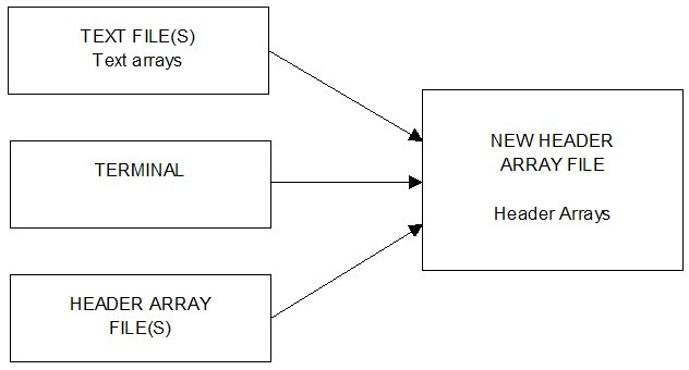
54.2 Modifying an existing header array file [gpd4.3.4]
One very common need for GEMPACK users is to modify data on an existing Header Array file. The arrays on the file cannot be edited directly; instead they are copied from the old existing file to a work array in memory. Here the data values in the array can be changed and finally can be written as Header Arrays to the new file. As shown in Figure 54.2, extra arrays can also be added from extra Header Array files (not just the old file) and from extra text files.
Figure 54.2 Modifying an existing header array file

Arrays on the old file which are not modified can be conveniently copied directly to the new Header Array file as a block.
Note that unlike some other packages (such as word processors or spreadsheets), MODHAR does not actually modify the existing Header Array file. Rather, MODHAR leaves it unchanged and creates a new Header Array file containing the changes you make. (For this reason, the new file should be given a different name from that of the existing one.)
54.2.1 Adding arrays from other files using MODHAR [gpd4.3.4.1]
MODHAR includes simplified procedures (via the commands at and ah) for adding arrays from text files (including spreadsheets1), or from extra header array files.
Using the format of GEMPACK text data files described in chapter 38 you can
- add several arrays from the same text file.
- include on text files the header and long name associated with each array (see section 38.1.4), and read them in with the array. This makes it a quick and simple procedure to read in all the arrays on a text file at once. Alternatively you can skip over arrays on the text file if you don't want them included on the new Header Array file.
- specify the order of data on text files as row-order, column-order or spreadsheet. The aim of this is to make it easy to transfer arrays of data between spreadsheets and Header Array files since one of the most convenient ways of editing data is on a spreadsheet.
54.3 Using MODHAR commands [gpd4.3.5]
MODHAR is a command-driven program and is easy to use. The menus of possible actions clearly state the tasks that you can currently perform.
MODHAR commences with the usual sort of GEMPACK options screen (as described in section 48.3). Then you are asked if the new file to be created is to be based on an old (that is, an existing) file.
Old or New File
If you are modifying an old file, respond 'y', and you will then be asked for the name of the file you wish to modify.
Otherwise (that is, you are creating a new file), respond 'n'.
Note that any references below to the "old file" are only relevant in case (i) above.
The MODHAR Command Menu offers the following commands:
Table 54.1 MODHAR commands
| ah | add one or more arrays from Header Array file |
| ds | define sets for adding arrays from a text file |
| at | add one or more arrays from text file |
| da | delete one or more arrays from old file |
| ra | restore one or more deleted arrays from old file |
| mw | modify data from the original file and write it on the new file |
| aw | add new data and write it on the new file |
| ex | exit, saving the new Header Array file |
| q | quit, without saving the new Header Array file |
| lh | list the headers, their status and size of associated arrays |
| oh | show one header, its status and size of associated array |
| ch | change a header name |
| eln | examine a long name |
| cln | change the long name associated with a header |
| ? | help |
MODHAR commands fall into four groups
- Commands for simply adding arrays to the new file ah, at, ds. [These are documented in section 54.4 below.]
- Commands for carrying out operations on headers or long names lh, oh, ch, eln, cln, da, ra. [These are documented in section 54.5 below.]
- Commands for complicated modification or addition of data on arrays from the old file, terminal or other files mw, aw. [These are documented in section 54.6 below.
- Exit commands ex or q. [These are documented in section 54.7 below.]
54.4 Commands for creating a new header array file [gpd4.3.6]
When MODHAR is being used to create a new Header Array file, it is usually just a matter of transferring data from elsewhere (text files, other Header Array files or input from the terminal) to the new Header Array file. This process is illustrated in Figure 54.4 where you can see that this can be accomplished using the MODHAR commands at, ah and aw. Once all the desired data has been added, you use the exit command ex (see section 54.7.1 below) to complete the task.
Figure 54.3 Commands for creating a new header array file
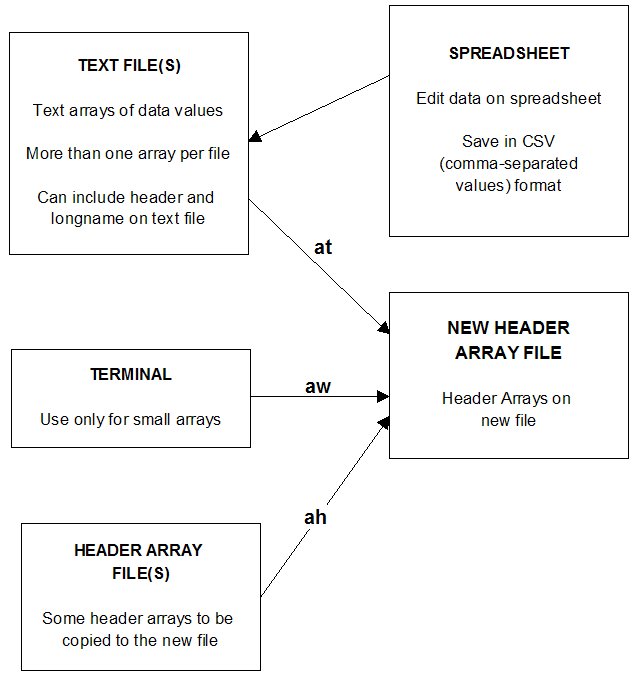
54.4.1 Commands for modifying an existing header array file [gpd4.3.6.1]
Here you may need to use the full range of MODHAR commands, as illustrated in Figure 54.4.1.
Although you are "modifying an existing Header Array file", the old file is not modified or changed. We just mean that you start with an existing Header Array file. A new file is created containing the arrays that you ask to be transferred from the existing file to the new file.
Figure 54.4 Commands for modifying an existing header array file
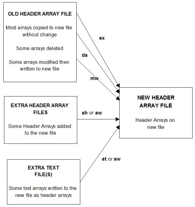
54.4.2 Commands for adding arrays to the new file [gpd4.3.6.2]
From an extra Header Array file
| Menu Choice | ah | add one or more arrays from a Header Array file |
Menu choice ah provides a simple procedure for adding complete arrays from an extra Header Array file. This extra file has arrays in header array format (so is a binary file). [Menu choice at provides a similar procedure for text files.]
After choosing ah, you will be asked for the name of the extra Header Array file. MODHAR displays the list of headers on the extra file and you are given the choice of adding
| [a] | all of the headers on the file |
| [L] | some of the headers (list ones to add) |
| [m] | most of the headers (list ones to omit) |
| [n] | none of the headers. |
For the choice [a] (which is the default here), the program adds ALL the arrays on the extra file to the new file. However, if the header of one of the arrays on the extra file is the same as that for an array already on the new file or for an array on the old file (but not deleted), the program will omit this array since adding it would cause duplicate headers on the new file.
For the choice [L], you supply a LIST of headers of arrays on the extra file to add to the new file. All other arrays on the extra file will be ignored. Again the program checks for duplicates and will tell you whether that header is already on the new or old file. If a duplicate is found, this array will not be added to the new file. Giving a carriage-return instead of a header ends the list of headers.
For the choice [m], the programs add MOST of the arrays on the extra files. You list the headers that you want to OMIT. A carriage-return ends the list.
For the choice [n], NONE of the arrays on the extra file are added. This gives a way out if you have chosen the wrong filename or if you just want to see what is on another file apart from the one you are modifying.
Example using the LIST option
The following example gives responses for adding arrays with headers 'EEEE' and 'FFFF' to the new file from an extra Header Array file.
ah ! add one or more arrays from Header Array file
extra_header.har ! name of extra file
L ! list ones to add
EEEE ! header of array to add
FFFF ! header of array to add
! carriage_return to end list to add
lh ! list headers
Headers 'EEEE' and 'FFFF' have been written to new file. The long names on the new file are the same as for these arrays on the extra file.
From a text file
| Menu Choice | at | add one or more arrays from a text file |
Menu choice at provides a simplified way of converting one or several arrays of data on a text file to header arrays and writing them to the new file in header array (that is, binary) form. [Menu choice ah provides a similar procedure for Header Array files.]
After choosing at, you supply the name of the extra text file and then are given the choice of adding
| [a] | all of the data arrays on the file |
| [s] | some of the arrays |
| [n] | none of the arrays |
For the choice [a] (which is the default here), all of the arrays are added. If a valid header, and (optionally) a long name, are given in the "how much data" information (see chapter 38) for an array, MODHAR will convert the text arrays read in to header array format and write them to the new file with the given header.
If the header is not read in from the text file with the array, or is not a valid choice, or duplicates a header on the old or new file, you will be asked to provide a valid header for this array.
For the choice [s], MODHAR reads in the arrays one by one and displays the type, dimensions and, if given on the text file, the header and long name.
You have the choice of
- accepting the header name with a carriage-return,
- giving a different header for this array, (type in the new header eg ABCD),
- skipping over this array (type XXX), or
- ending the reading of data from this file (type XXQ).
For 1 and 2, once a valid header is given, you are asked for the long name (if one is not specified in the text file) and then the array is written as a header array to the new file while for 3, no array is written. After this MODHAR goes on to read the next array till the end of file is reached or XXQ is input to end reading this text file.
For choice [n], none of the arrays are added and you are returned to the main menu.
Example using the SOME option
The following example gives responses for adding headers 'GGGG' and 'HHHH' to the new file from an extra text file.
at ! add one or more arrays from text file
extra_text.txt ! name of extra file
s ! add some of the arrays
! carriage_return to add 'GGGG'
HHHH ! no header specified on the text file - input header
second array ! long name for array
XXQ ! XXQ to end list to add
lh ! list headers.
Headers 'GGGG' and 'HHHH' have been written to new file.
The text file was as follows:
2 3 real row_order header "GGGG" longname "first array" ; 4.0 2.0 1.0 1.0 6.0 8.0 6 integer ; 1 2 3 4 5 6 3 strings length 5 header "xyza" ; abcde pqr 11223
The appropriate format for the text arrays on the text file is described fully in chapter 38.
Define Sets
| Menu Choice | ds | define sets for adding arrays from a text file |
Menu choice ds provides way to read in the element names in sets used in adding set and element information to arrays read in from a text file. A full example of this process is given in section 75.0.3.4.
The sole purpose of the ds command is to define certain set and element names which will then be used to add set and element labelling (see section 5.0.3) to arrays of data added from text files via the at command. See section 75.0.3.4 for more details about this.
You need to select ds and add the set information before you choose at to add the arrays from the text file. The names of the set elements are initially prepared on a Header Array file as arrays of character data.
On selecting the menu item ds, you will be asked for the name of the Header Array file containing the element names for the sets. Then you will be asked for a list containing the set name and the Header of the array which lists the element names for that set. (A carriage return ends the list.).For example, suppose the elements of set COM are in the array with header "CCCC" and the elements of set IND are in header "IIII" the list would be
COM CCCC IND IIII <carriage-return>
If on the Header Array file containing the element names, you have arrays with longname starting with the word "Set" and with the following word the name of the set that you are defining eg COM, for example, if the longnames of two of the Header Arrays are
"Set COM Commodities"
"Set IND Industries"
then MODHAR will select these Headers and associate them with the sets COM and IND respectively. You will be asked if you wish to add all sets with longnames of this type as a group without your having the enter the names of the sets and associated Headers one by one.
Note that the arrays used to define sets are not written explicitly to the new file. They are just stored in memory and used to add set and element labelling to other arrays.
54.5 Operations on headers or long names [gpd4.3.7]
Initially MODHAR assumes that all arrays on the old file will be copied to the new file. To ensure headers on the new file are unique, MODHAR checks for duplicates in the new header list assuming
- all (non-deleted) arrays on the old file will be included on the new file.
Of course,
- headers of all arrays already written to the new file are included in the list of new headers.
(Initially, the "new" header associated with each array on the old file is its header on that file, but this can be changed using the ch command.)
Listing Headers
| Menu Choice | lh | list the headers, their status and size of associated arrays |
| oh | show one header, its status and size of associated array |
Menu option lh shows the complete list of headers while oh gives the same information for just one header. Status refers to whether the header is on the old file, the new file, an extra file or in memory during modification (mw). Old and new header names are given. In using oh, the header given should be the new header name of the array in question.
The following table is a sample of the output from lh.
No. Header Status Data Size Size
Old New type old new change?
1 AAAA ABCD On old file real 2 x 2 2 x 2 no
2 BBBB BBBB On old file int 6 6 no
3 CCCC CCCC On old file real 2 x 5 2 x 5 no
4 DDDD DDDD On old file real 2 2 no
5 EEEE EEEE Deleted int 3 x 4 3 x 4 no
6 FFFF FFFF Deleted char 3 strs,len 5 3 strs,len 5 no
7 GAMM GAMM ON NEW FILE real 1 x 2 1 x 2 no
8 PROD PROD ON NEW FILE real 2 x 2 2 x 2 no
9 AAAA AAAA ON NEW FILE int 6 6 no
10 FFFF FFFF ON NEW FILE int 4 4 no
11 (TM) GGGG ON NEW FILE real 2 x 4 x 7 2 x 4 x 7 no
12 CCCC HHHH IN MEMORY real 2 x 5 6 x 5 YES
The original Header Array file contained arrays with headers AAAA, BBBB, CCCC, DDDD, EEEE, FFFF. Header AAAA was changed to ABCD using ch and arrays EEEE and FFFF were deleted using da.
Command ah and an extra Header Array file were used to add GAMM, PROD, and a new version of AAAA and FFFF.
Array GGGG was added from the terminal using command aw (see section 54.6). Command aw is currently being used to modify array CCCC from the old file to a new array with header HHHH; the size of this array has been increased from size 2 x 5 to 6 x 5.
Changing Header or Longname
| Menu Choice | ch | change a header name |
| eln | examine a long name | |
| cln | change a long name associated with a header |
Menu option ch is used to change a header on the old file to a new different header. At the end when the array corresponding to this header is copied to the new file (see section 54.7), this array will have the new header associated with it.
Option eln is used to display the long name associated with a header and cln is used to change the long name to a new value. A "long name" associated with a Header Array is a character string of up to 70 characters which can be used to describe the array in more detail than the 4 character header.
Deleting Arrays
| Menu Choice | da | delete one or more arrays from the old file |
To delete one or more arrays, choose the menu item da. You will be asked for a list of headers associated with arrays on the old file which you wish to delete. (These headers should be the names on the old file.) The associated arrays are marked 'deleted' and at the end of the program (when you exit) are not copied across to the new file. (They are, of course, not actually deleted from the old file, which is never changed by MODHAR.)
Only arrays on the old file can be deleted. (Arrays already written to the new file cannot be deleted.)
The header associated with a new array (added via at, ah or aw commands) cannot be the same as the new header associated with one of the un-deleted arrays on the old file. (This is because MODHAR must not allow duplicate headers on the new file.) In such a case you can either delete the old array using da or else change the new header associated with the old array using ch.
So, in summary, there are two reasons you might have for using da.
To mark an old array as deleted so it will not be transferred to the new file when you exit MODHAR .
To clear the header name so you can associate it with another array of data.
Example of case (ii) above
For an old file containing arrays with headers 'AAAA', 'BBBB', 'CCCC', we wish to remove the old arrays 'AAAA' and 'CCCC' and insert from an extra Header Array file, new arrays with headers 'AAAA', and 'CCCC'. After opening the old and new files, give the following responses.
da ! delete one or more arrays from the old file
AAAA ! header on old file to delete
CCCC ! next header to delete
! carriage_return to end the list
ah ! add one or more arrays from Header Array file
extra_header.har ! name of extra file
L ! list ones to add
AAAA ! header on extra file to add
CCCC ! next header to add
! carriage return to end the list
lh ! list headers to see the result
Restoring Deleted Arrays
| Menu Choice | ra | restore one or more deleted arrays on the old file |
If an array has been deleted from the old file, you can restore it using the menu choice ra. You will be asked for a list of headers to restore to the list of headers of arrays to be copied across to the new file from the old file on exit.
As with all cases when a header is added to the list of headers to be added to the new file, MODHAR checks for duplicates which might occur on the new file (including those to be copied from the old file). If the program finds a possible duplicate, you will be asked to supply a new header for the array you are restoring.
54.6 Commands for complicated modification or addition [gpd4.3.8]
Modify Write or Add Write
| Menu Choice | mw | modify data from the old file and write it on the new file |
| aw | add new data and write it to the file |
If you choose either mw or aw, a (secondary) MODHAR Sub-command Menu becomes active, offering the Sub-commands shown below.
Note that you should use command aw rather than at or ah if
- you want to modify the data read before writing it to the new file, or
- you want to enter the new data from the terminal.
54.6.1 MODHAR sub-commands for mw or aw [gpd4.3.8.1]
| m | modify the data (before writing it) |
| ed | examine part of the data (held in memory) |
| is | increase the size of the array |
| w | write (all of) the array to the new file |
| wp | write part of the array to the new file |
| a | abort this Sub-command, and go to the Command menu |
| lh | list the headers, their status and size of associated arrays |
| oh | show one header, its status and size of associated array |
| ch | change a header name |
| eln | examine a long name |
| cln | change the long name associated with a header |
| ? | help |
For users unfamiliar with the operation of MODHAR, use of the help command ? lists the current menu to the terminal screen. Subcommands lh, ah, ch, eln and cln operate in the same way as the command of the same name documented in section 54.5.
MODHAR gives a range of prompts depending on which Subcommand has been chosen. Generally, you name the header of an array to be modified. MODHAR reads the array into a work array in memory. You can then examine the data in this array ed, increase its size is or modify the data m by replacing parts of it or scaling its values.
When the modification of the array is complete, it is written to the new file using w or wp. Once an array is written to the new file it cannot be further modified.
54.6.2 Examples [gpd4.3.8.2]
Some examples may be useful to indicate the operation of MODHAR and the types of questions MODHAR may ask the user.
Example 1 Source of data
When you want to add an array to the new Header Array file, a series of MODHAR prompts will ask you where the array data comes from. The possibilities are :
- directly via input by the user at the terminal,
- from a formatted text file,
- from the old Header Array file upon which the new Header Array file is based or
- from some other Header Array file.
Example 2 Terminal Input
When you are typing in the actual values for a new array to be added to the new Header Array file, MODHAR will ask a series of questions :
what type of data is being added - real, integer or character values,
the number of dimensions of data,
the actual dimension sizes,
the values for the array data are prompted for, with a clear indication of their position in the array. For example, for a 6x3x4 real array, you will receive prompts of the form:
Please enter the 6 values for positions (1-6, 2, 3)
Example 3 Modifying the data
When modifying an array that has been just read by MODHAR (including an array whose values have just been input by the user), MODHAR will ask such questions as:
- how much of the array is to be modified ? - possibilities are one single entry, a few entries, a rectangular sub-array or the whole array.
- is the modification a scaling of the current values, an addition to the current values, or a replacement?
- are all entries to be modified in the same way ? i.e. either scale all values by the same factor, or add the same amount to all values, or replace all values with the same replacement value.
- if the modification is different for different values, are the individual modification (scaling, adding or replacement) values read from the terminal, from a text file, from the old Header Array file upon which the new Header Array file is based or from some other Header Array file ?
Example 4 Modifying a sub-array on an old Header Array file
This example gives full responses for a run of MODHAR which modifies an array on the old file before writing it to the new file.
-
First the array dimensions are increased from 2 x 3 to 4 x 4.
(The new positions initially contain zero values.) - Then two new data values are added as a subarray in positions (3->4,4) from data input from the terminal.
The old array 'abcd' was
4.0 2.0 1.0 1.0 6.0 8.0
After modification the new array will be
4.0 2.0 1.0 0.0 1.0 6.0 8.0 0.0 0.0 0.0 0.0 3.0 0.0 0.0 0.0 5.0
User input would be:
<carriage-return> ! carriage return to end option selection y ! based on an old Header Array file old_file.har ! Name of old Header Array file new_file.har ! Name of new file lh ! list headers of arrays on old file mw ! modify an array on old file and write it to new file abcd ! header of array to be modified is ! increase size of array 1 2 ! increase dimension 1 by 2, that is, from 2 to 4 2 1 ! increase dimension 2 by 1, that is, from 3 to 4 end ! end selection of dimensions to increase m ! modify this array before writing to new file r ! replace some parts of the array data s ! modify a subarray 1 3 4 ! select entries 3 to 4 in first dimension 2 4 4 ! select entry 4 in second dimension end ! end of selection of subarray (3-4,4) of size 2 x 1 g ! general matrix used to modify array t ! input modifying matrix from terminal 3.0 5.0 ! enter 2 values since array is of size 2 x 1 ? ! view menu for list of commands w ! write all the array to the new file n ! don't want to reuse data in memory ex ! exit saving the new header array file a ! all remaining arrays to be transferred = ! use old history without adding to it
54.6.3 Writing arrays to the new header array file [gpd4.3.8.3]
Once you have completed all modifications to an array, the array can be written to the new Header Array file. MODHAR gives you the choice of writing either the entire array (using the w Command) or only a rectangular sub-array of the entire array (using the wp Command). Before proceeding onto another array, you can also base an entirely new array on the most recently written array. In this way, any complicated modifications just performed for that array need not be repeated.
Note that, although there is an is Subcommand for increasing the size of an array, no ds ("Decrease the size") Subcommand is needed since you can decrease the size by only writing part of the array.
Example 5 Writing part of an array using wp
This example gives full responses for a run of MODHAR which
- examines part of an array using the ed command, and
- writes part of an array to the new file using the wp command.
Initially the array has dimensions 4 x 3 x 4 x 5 x 2.
On the new file, the sub-array written is
1 , 1 -> 3 , 2 , 2 -> 5 , 1 -> 2
The new array has dimensions 1 x 3 x 1 x 4 x 2.
User input would be
<carriage-return>! carriage return to end option selection y ! based on old file old.har ! old file name new.har ! new file name lh ! list headers on old file mw ! choose modify and write option JJJJ ! header of array to be modified ed ! examine data s ! examine a submatrix 2 1 3 ! second dimension elements 1-->3 3 2 2 ! third dimension element 2 4 2 5 ! fourth dimension elements 2-->5 5 1 2 ! fifth dimension elements 1-->2 end ! end of selection of submatrix ? ! list menu of options wp ! write part of the array to the new file 2 1 3 ! write second dimension elements 1-->3 3 2 2 ! third dimension element 2 4 2 5 ! write fourth dimension elements 2-->5 5 1 2 ! write fifth dimension elements 1-->2 end ! end selection - written 1 x 3 x 1 x 4 x 2 array n ! don't reuse data in memory lh ! list headers ex ! exit saving the new file a ! all remaining arrays to be transferred Jill ! name as part of history 12 -1-00 ! date (Only prompted for on some machines) Example of selecting part of an array **end y ! accept history for new file
54.6.4 Option ADD when modifying data in MODHAR [gpd4.3.8.4]
When you modify the data on an array using MODHAR, you were offered the options:
| r | replace |
| s | scale |
| a | add |
With the last, add, option, the numbers entered are added to the values at the original header. Of course you can subtract values by adding negative values. (For example, if you add -2 to each entry of a matrix, this is the same as subtracting 2 from each entry.)
54.7 Finishing up [gpd4.3.9]
If the new Header Array file was based on an existing, Header Array file, then, when you have finished either adding any new arrays or writing any modified arrays to the new Header Array file, MODHAR gives you the option of copying unchanged, some or all of the arrays from the old file that have not yet been transferred to the new file.
Suppose, for example, that you wish to copy an existing Header Array file containing 100 arrays, only one of which needs to be modified, then you only need to access explicitly the array to be modified. Once the single modified array has been written to the new Header Array file and you enter the ex command to exit MODHAR, MODHAR will ask if you want to copy some or all of the untouched 99 arrays from the old Header Array file across to the new Header Array file. In this way, you are saved from having to access explicitly any array that requires no modifications.
54.7.1 Exit commands [gpd4.3.9.1]
Exit or Quit
| Menu Choice | ex | exit, saving the new Header Array file |
| q | quit without saving the new Header Array file |
When you have finished adding, deleting and modifying arrays, menu choice ex is the way to exit MODHAR if you want to save the newly created Header Array file. Choice q aborts the process and deletes the new file.
If the new Header Array file was based on an existing Header Array file and you give command ex, MODHAR gives you the option of copying unchanged some or all of the arrays from the old file which have not previously been transferred to the new file and have not been deleted using da. The choices are:
| [a] | ALL remaining arrays to be transferred |
| [L] | LIST headers of arrays to be transferred |
| [m] | MOST of the arrays (List those not transferred) |
| [p] | Respond to PROMPTS to enter which to transfer |
| [n] | NONE of the arrays to be transferred. |
[a], [L], [m], and [n] are similar to those in menu item ah.
For the choice [a], the program adds ALL the non-deleted arrays on the old file to the new file.
For the choice [L], you supply a LIST of headers of arrays on the old file to add to the new file. All other arrays on the old file will be omitted. Giving a carriage-return instead of a header ends the list of headers.
For the choice [m], MODHAR adds MOST of the arrays on the old file. You list the headers that you want to OMIT. A carriage-return ends the list.
For the choice [n], NONE of the remaining arrays on the old file are added.
For the choice [p], MODHAR prompts you with the header names of undeleted arrays on the old file and you choose from the following list of actions:
| [y] | Transfer this array to the new file. |
| [n] | Do NOT transfer this array. |
| [r] | Transfer this and ALL REMAINING arrays. |
| [q] | Do NOT transfer this or ANY REMAINING ARRAYS. |
| [?] | Display this menu again. |
After transferring the requested arrays, a list of headers is produced showing the status and sizes of the arrays on the old and new files.
54.7.2 History of the new file [gpd4.3.9.2]
Finally you are asked to add to the history by supplying your name and any notes you wish to append to the current history about what changes have been made in this run of MODHAR. (On some machines you may also be asked to input the date.)
If you don't want to add to the history in this way, you can choose from
| [-] | ignore any old history. (Start the history with a fresh slate - type in your name and a new history.) |
| [=] | to take any old history (no new). (Copy the old history to the new file without adding to it.) |
| [0] | to have no history on the new file. |
54.8 Complete example of a MODHAR run [gpd4.3.10]
The following example gives all responses for a MODHAR run. If you want to try it yourself, create the following three files (either using option at and taking data from a text file, or using option aw and giving input from the terminal.)
Initially you need
- An old file 'old_file.har' containing arrays with headers 'AAAA', 'abcd', 'EEEE' and 'FFFF'
- An extra file 'moupd.har' containing arrays with headers 'prod' and 'gamm'
- A second extra file 'extra_header.har' containing an array with header 'AAAA'.
User input
<carriage-return> ! carriage return to end option selection y ! based on an old file old_file.har ! name of old file new_file.har ! name of new file lh ! list headers on old file ah ! add arrays from extra Header Array file moupd.har ! name of extra file L ! list headers of arrays to add prod gamm <carriage-return>! carriage return to end list lh ! list headers to see 'prod' and 'gamm' on new file da ! delete arrays on old file AAAA ! header of array to delete FFFF ! header of array to delete <carriage-return>! carriage return to end list lh ! list headers to see deleted arrays 'AAAA' and 'FFFF' on old file ah ! add arrays from an extra Header Array file extra_header.har ! name of extra file L ! list headers to add to new file AAAA ! header to transfer (permitted since old 'AAAA' is deleted) <carriage-return> ! carriage return to end list lh ra ! restore array deleted from the old file AAAA ! this is the original header on the old file BBBB ! necessary to enter a new header because 'AAAA' is on new file <carriage-return> ! carriage return to end list to restore lh aw ! add a new array and write it to the new file o ! from the old file cdef ! header of array on old file fghi ! 'cdef' is on old file so a new header is needed 'fghi' w ! write array to new file n ! don't reuse array in memory lh ex ! exit saving the new file a ! all remaining (non-deleted) arrays to be copied to new file Jill ! add to history on new file 29/9/99 ! Date (Only prompted for on some machines) Example for MODHAR **end ! end of history y ! confirm history before adding
After running this example, on the new file are arrays with headers 'BBBB' (was 'AAAA' on old file), 'abcd', 'cdef', 'EEEE'. All these were originally on the old file.
Also on the new file are arrays 'gamm' and 'prod', and the new version of 'AAAA' from extra Header Array files.
The new file also contains a second copy of array 'cdef' from the old file now renamed 'fghi'.
54.9 Text files [gpd4.3.11]
MODHAR allows the use of prepared text files to input a variety of data, the data values of an array, the scaling factors to be applied to values in an array, or the replacement values for arrays or subarrays.
A text file is a file which can be viewed or edited with a text editor. Text data files which GEMPACK programs can read have a particular format and are referred to as GEMPACK text data files. Full details of preparing arrays for GEMPACK text data files are given in chapter 38.
In MODHAR when using option choice at, the GEMPACK text file can contain more than one array of data. In other parts of MODHAR, only one array should be given on each text file.
54.10 Example: Constructing the header array data file for Stylized Johansen [gpd1.4.2]
You have looked at the Header Array data file SJ.HAR for Stylized Johansen in section 3.4.3 above. In this section we take you through the steps to construct that file SJ.HAR. We recommend that you carry out these steps on your own computer.
The routine way of creating a Header Array data file is to first create one (or more) text data files which between them contain the arrays (or matrices) of data. [These text files can be created via an editor or from spreadsheet output or, occasionally, by writing a program.] Then it is easy to run MODHAR to create a Header Array file containing these arrays of data at the appropriate header (as stated in the TABLO Input file). We illustrate this for Stylized Johansen below.
As you have seen in section 4.2.1 above, we need three arrays of data for DVCOMIN, DVFACIN and DVHOUS; these are of size 2 x 2, 2 x 2 and 2 respectively. The matrices of data required are as shown in the data base in Table 3.1 of section 3.1.1 above, namely
| DVCOMIN | 4.0 | 2.0 |
| 2.0 | 6.0 | |
| DVFACIN | 1.0 | 3.0 |
| 1.0 | 1.0 | |
| DVHOUS | 2.0 | 4.0 |
Step 1 — Create a GEMPACK Text File Containing the Data
The first step is to create a text file containing the data. For each array of data on a text file, there are two parts:
- the "how much data" information, and
- the actual data.
The "how much data" information begins with the size of each dimension (or argument on the TABLO Input file) of the array. For example. this is just '2' for DVHOUS and is '2 2' for DVCOMIN since it is an array of size 2 x 2. Then, on text files for input to MODHAR, it is usual to include the header and long name which will be associated with the array on the Header Array file to be created, following the syntax
header "<header>" longname "<long name>"
The header must agree with that specified for the relevant READ statement on the TABLO Input file (see section 4.3.3 above).
The name of the Coefficient usually associated with this data can be indicated following the syntax
Coefficient <coefficient name followed by set arguments>
Finally, the "how much data" information must end with a semi-colon ';'. For example, the "how much data" information for DVCOMIN is
2 2 header "CINP" longname
"Intermediate inputs of commodities to industries - dollar values"
coefficient DVCOMIN(SECT,SECT);
(The long name, which can describe the data in some detail, and can be up to 70 characters long, is enclosed in quotes " " and must all be on one line of the file. It cannot be split over two lines. The coefficient name, which is optional, is the coefficient in the associated TABLO Input file normally associated with this data — see section 38.1.5.)
The actual data is, by default, in ROW order, with each row starting on a new line of the file.
For example, for DVFACIN, the data part is
1.0 3.0 ! first row of the matrix of data 1.0 1.0 ! second row of the matrix of data
The full text data file for the Stylized Johansen model is shown below.
Text Data File SJDAT.TXT for Stylized Johansen
! Text data file (usually called sjdat.txt) which can be used ! with MODHAR via the 'at' option to create a Header Array ! file (usually called SJ.HAR) to be the file with logical ! name 'iodata' referred to in the TABLO Input ! file (usually called sj.tab) for the Stylized Johansen model. ! The data are as set out in Table 3.1. ! ! DVCOMIN - dollar values of commodity inputs to current production ! 2 2 header "CINP" longname "Intermediate inputs of commodities to industries - dollar values" coefficient DVCOMIN(SECT,SECT) ; 4.0 2.0 2.0 6.0 ! ! DVFACIN - dollar values of primary factor inputs to current production ! 2 2 header "FINP" longname "Intermediate inputs of primary factors - dollar values" coefficient DVFACIN(FAC,SECT) ; 1.0 3.0 1.0 1.0 ! ! DVHOUS - dollar values of household use of commodities ! 2 header "HCON" longname "Household use of commodities - dollar values" coefficient DVHOUS(SECT) ; 2.0 4.0 ! ! End of file
The text after the exclamation marks contains comments. Such comments, which will be ignored by the program MODHAR when it reads these files, can come anywhere in the file.
The comments, which can make the file self-documenting, follow the same syntax as for comments in terminal input or Stored-input files. That is, they start with a single exclamation mark '!' and end at the end of the line. A comment can be continued over several lines by putting an exclamation mark in the first column of the next line. [See section 48.2 for more details.]
The actual data read by MODHAR is shown in the box above in bold font.
Note that the file SJDAT.TXT shown above is usually supplied with GEMPACK and so should be in the relevant directory on your computer. [If not, you will have to create this text file using a text editor.] We suggest that you open this file in your text editor and find the three arrays of data and their associated "how much data" information. You will use this file in Step 2 below.
Step 2 — Run MODHAR to Create a Header Array File
The 3 arrays of data can be put on to a GEMPACK Header Array file by running the program MODHAR. We reproduce below the commands for running MODHAR to do this.
We encourage you to actually run MODHAR using this input to make your own copy of the data file for Stylized Johansen.
To use WinGEM, first ensure that both default directories point to the directory (usually c:\sj) in which you put the files for Stylized Johansen (see section 3.4.2 above). Click on menu item Programs and select item Run programs interactively and then click on MODHAR . The program MODHAR will begin to run in a DOS box. Give the responses shown in the box below.
If you are working at the command prompt, change into the directory in which you put the files for Stylized Johansen. Then type modhar and then enter the responses in the box below.
[After each response (on the left), we have given a comment, which starts with an exclamation mark '!'. When running the program, you should not type in the exclamation mark or the following comment - just type in the text at the left. The first response is a carriage-return or ENTER.]
Input for MODHAR to recreate data file for Stylized Johansen
<carriage-return> ! Use default program options
n ! Not based on old file (we are creating a new one)
sj2.dat ! Name of file to be created
! (Now comes the input saying you wish to add all arrays
! from the text file 'sjdat.txt'.)
at ! Add arrays from a text file
sjdat.txt ! The name of the text file
a ! Add all arrays from this file
! (Now the end of the program)
ex ! Exit (There is no more data to add.)
<Your name> ! Your name
Standard input-output data for the Stylized Johansen model. ! History
**end ! end the history
y ! Yes, this history is what I wanted
When MODHAR has finished, you may wish to check that the file SJ2.DAT has been created.2 Use ViewHAR to examine the data on SJ2.DAT.
As you can see from this, it is easy to use MODHAR to create a Header Array file with any number of arrays of data (once you have prepared the text file containing the data). It is also easy to prepare a file which contains all these inputs since the responses required are easily predicted. Such a file is called a Stored-input file (see section 54.11 below for an example).
Step 3 — Run a Simulation with Zero Shocks to Add Set and Element Labelling
Ideally Header Array files should include set and element labelling (see chapter 5.0.3). Then, when the data on these files is examined (for example, via the programs SEEHAR or ViewHAR, whose use has been described in chapter 3 above), this labelling makes it clearer which commodities (etc) the data correspond to. The file SJ2.DAT produced in Step 2 above does not yet have this labelling.
There are various ways of adding the labelling. Perhaps the simplest is to run a simulation in which zero shocks are given. The updated data will then be identical (in values) to the original data. However, the software adds set and element labelling to this updated data.3 To do this for the Stylized Johansen data, you can modify the Command file SJLB.CMF to change the shock to p_XFAC("labor") to 0 (rather than 10). Also change the name of the pre-simulation data to SJ2.DAT (the file created in Step 2 above) and the solution method to Johansen. You should also change the name of the Command file to something different — say SJLABEL.CMF.4 You should also change the name given to the updated data in that file, perhaps changing the relevant line to..updated data file iodata = sjlabel.dat ;..Then carry out a simulation (as in the Step 2 part of section 3.5.2 or 3.5.3 taking inputs from this Command file SJLABEL.CMF. You can then use the "updated" data file SJLABEL.DAT in place of SJ2.DAT since it has the same data and also set and element labelling.5 Alternative to Step 3 — Write a TABLO Input file
You can also add set and element labelling (row and column labels) to the Header Array file by writing a very simple TABLO Input file.
For example, to label the Header Array "HCON" which you want to label with the sectors (s1, s2), read in the unlabelled array and write it to the new Header Array file. The resulting array on the new data file will be labelled with the element names in the set SECT.
SET SECT # Commodities # (s1, s2) ; . FILE data # Original data - Header array file # ; FILE (NEW) new_data # Base data - Header Array file # ; COEFFICIENT (all,i,SECT) DVHOUS(i) ; READ DVHOUS FROM FILE data HEADER "HCON" ; WRITE DVHOUS TO FILE new_data HEADER "HCON" ; TABLO Input File SJLAB1.TAB for Adding Set and Element Labelling
To do this, create a TABLO Input file SJLAB1.TAB containing the statements above. Also create the Command file SJLAB1.CMF containing the lines below.
Auxiliary files = sjlab1 ; ! Input data files file data = sj2.dat ; ! Output (labelled) file file new_data = sjlab1.har ;
Command file SJLAB1.CMF for Adding Set and Element Labelling
Run TABLO to process TABLO Input file SJLAB1.TAB as in the Step 1 part of section 3.5.3 above to produce output for GEMSIM (for simplicity). Then run GEMSIM taking inputs from the Command file SJLAB1.CMF as in the Step 2 part of section 3.5.3 above.6 This should produce the new Header Array file SJLAB1.HAR containing just header "HCON" and labelled DVHOUS data.
Use ViewHAR to look at the data in SJLAB1.HAR and to check that there are set and element labels.
54.11 Example: Modifying data using MODHAR [gpd1.4.3]
Once you have created the Header Array file or files for your model, you may wish to change the data. You can do this either by editing the text file used with MODHAR to create the original file (as in section 54.10 above) and then re-running MODHAR, or by running MODHAR to modify the data on the Header Array file directly. Below we show you how to carry out this second alternative.
Example 1 — Replacing one array on an existing file
Below we give a simple example of replacing the data at header "CINP" with a modified version of the data. The modified array is on a Header Array file called SJNEWC.HAR which is supplied with the GEMPACK examples and so should be in the directory in which you put the Stylized Johansen files (see section 3.2 above).
We suggest that you run MODHAR (as in Step 2 of section 54.10 above) and give the following responses.. The new file (SJMOD.DAT) created will have this new version of the array incorporated in it.
When running MODHAR, it is a good idea to make a Stored-input file containing the MODHAR responses using the program option sif, as shown below where you will create the Stored-input file modsj.sti. If you want to rerun MODHAR later, to carry out the same set of operations, you can use the Stored-input file instead of typing in all the responses again. See section 48.3 for more details about Stored-input (STI) files.
Responses to MODHAR to modify data from Stylized Johansen
sif ! Save inputs on Stored-input file modsj.sti ! Name of Stored-input file <carriage-return> ! Use default program options y ! Is based on existing file SJ.HAR ! Existing file (as supplied with GEMPACK) sjmod.dat ! New file to be created, containing modified data ? ! List commands da ! Delete array CINP ! Name of Header to delete <carriage-return> ! Finish list of headers to delete ah ! Add header sjnewc.har ! Name of file containing new array L ! List headers to add CINP ! Header of new modified array on newdata.har <carriage-return> ! Finish list of headers to add ? ! List commands ex ! Exit a ! Transfer all other arrays from the old file <your name> ! Name of person modifying the file Replaced header CINP with new version ! History from file sjnewc.har ! History **end ! End of history
When MODHAR finishes, use ViewHAR or SEEHAR to look at the data in the file SJMOD.DAT you have just created. Check that the data at header "CINP" has changed from that at this header in SJ.HAR and is the same as the data at header "CINP" in SJNEWC.HAR.
We have begun the MODHAR run above with response "sif" in order to store these responses on the Stored-input file modsj.sti. Suppose you find you have made a mistake in preparing the data on the file SJNEWC.HAR and need to replace the array "CINP" again at a later time. To rerun MODHAR to repeat this process of replacing the array "CINP", you can then take advantage of the fact that file modsj.sti was already created to simply type in at the command prompt
modhar -sti modsj.sti
(see section 48.5 below).
Example 2 — Modifying one data item in an array
This is an example showing how you can use MODHAR to modify data on the Header Array file produced in section 54.10 above. Suppose that you want to change the input-output data base for Stylized Johansen so that industry 2 uses an input of 7 (million) dollars' worth of commodity 2 (rather than 6 as in the standard data in section 3.1.1 above). Note that the data base will still be balanced after this single change.
(However it hardly ever makes sense to change just one data item in a data base because often the data base is no longer balanced after the change.)
We suggest that you run MODHAR (as in Step 2 of section 54.10 above) and give the following responses.. The new file (SJMOD2.DAT) created will have this change incorporated in it.
Note that Stored-input file repsj.sti will be created in this run. You could use it to repeat the run later, if necessary.
Example of responses to MODHAR to modify data for Stylized Johansen
sif ! Save inputs on Stored-input file
repsj.sti ! Name of Stored-input file
<carriage-return> ! Use default program options
y ! Is based on existing file
SJ.HAR ! Existing file (as supplied with GEMPACK)
sjmod2.dat ! New file to be created, containing modified data
(A typical set of responses to change data in one array)
mw ! Modify and write one array
CINP ! Header whose associated data is to be modified
m ! Modify the data
r ! Replace (not scale)
o ! One entry
2 2 7.0 ! Replace entry in row 2 and column 2 by value 7.0
w ! Write the modified data
n ! Do not use this as basis for another array
(Now exit, transferring unchanged the other 2 arrays)
ex ! Exit
a ! Transfer all other arrays
<Your name> ! Your name
Modified input of commodity 2 to industry 2 ! History
from 6 to 7. ! History
**end ! End of history
y ! Yes, this is what I want
When MODHAR finishes, use ViewHAR or SEEHAR to look at the data at header "CINP" in the new file SJMOD2.DAT. Check that the altered value of 7 is shown.
More complicated changes would require more complicated responses. But the general idea should be clear from the above. Note that, when you actually run MODHAR, it gives you information confirming initial values and new (modified) ones.
Complete documentation for MODHAR is given in chapter 54.
55 Ordering of variables and equations in solution and equation files [ordering]
Click here for detailed chapter contents
55.1 Ordering of variables [gpd2.4.15.2]
The order in which variables are declared in the TABLO Input file is also the order in which they are stored on the solution file — although ViewSOL usually displays them alphabetically. The solution file order also governs how variables occur in the columns of the Equations matrix (see section 3.12.1). This is only relevant if you are using SUMEQ (see chapter 79) to look at the Equations file.
55.1.1 Ordering of components of variables [gpd2.4.15.3]
This refers to the order, within a given variable, that the components of that variable appear in the Solution file or in the columns of the tableau or Equations Matrix (see section 3.12.1).
The order of indices in the variable declaration determines the component order, under the rule that the first index varies fastest, followed, in order, by each subsequent index.
For example, if the set IND has elements "car" and "food" and the set FAC has elements "labor" and "capital" and variable x3 is declared via
VARIABLE (ALL,i,IND)(ALL,f,FAC) x3(i,f) ;
then x3 has four components. The first is x3("car","labor"), the second is x3("food","labor") (because i varies faster than f), then x3("car","capital") and, finally, x3("food","capital").
Other examples are given in section 66.4.
The order of the quantifiers in the declaration has no bearing on the order of the components. Thus, if x3 above had been declared via
VARIABLE (ALL,f,FAC)(ALL,i,IND) x3(i,f) ;
the order of the components would be the same as described above.
55.2 Ordering of the equation blocks [gpd2.4.15.4]
The order of the equation blocks in the tableau or Equations Matrix (see section 3.12.1) is determined by the order in which they are declared on the TABLO Input file. You may need to know this if you are using SUMEQ (see chapter 79) to examine the Equations file.
55.2.1 Ordering of the equations within one equation block [gpd2.4.15.5]
The order of equations in a block is not very important. You only need to know it if you are checking the entries of the Equations file (via SUMEQ, for example).
The order of equations in a block is determined by the order of the quantifiers in the EQUATION statement. The index in the first quantifier varies fastest, followed, in order, by each subsequent index.
For example, if the set IND has elements "car" and "food" and the set FAC has elements "labor" and "capital" and equation EX1 is defined via
EQUATION EX1 #Example equation#
(ALL,i,IND)(ALL,f,FAC) x3(i,f) - y(i) = 0 ;
then there are four EX1 equations, corresponding to the elements of the sets IND and FAC as follows :
| IND value | FAC value | |
| First EX1 equation | "car" | "labor" |
| Second EX1 equation | "food" | "labor" |
| Third EX1 equation | "car" | "capital" |
| Fourth EX1 equation | "food" | "capital" |
56 SEENV: to see the closure on an environment file [gpd4.12]
Click here for detailed chapter contents
SEENV is a utility program to look at the closure on an Environment file, Solution file or LU file. Since all of these files are binary files, they cannot be examined directly, as you would a text file, or transferred to other operating systems. If you have used "swap" statements in setting up your closure, SEENV can be used to look at the resulting closure to check exactly which variables and components are exogenous, and which are endogenous. Variables which have been condensed out of the model do not occur in either list.
After giving the name of the file which contains the environment, and the name of the output text file, you specify the type of output that you would like on the output text file. The three possible types are:
- text suitable for including in a Command file to give the closure,
- a text file which can be used as a Spreadsheet Mapping file (see section 40.1),
- a text file containing Shock statements for the bottom of a Command file such as
Shock x1 = select from file xx.har header "ABCD" :
You must also choose whether you want just the exogenous variables, just the endogenous variables or both types (that is, all the variables in the (condensed) model).
56.1 Command file output [gpd4.12.1]
If you ask for Command file output and choose exogenous variables, the output will be a text file containing the key word "exogenous", followed by a list of exogenous variables, then a semicolon ; to end the exogenous statement, and then the completing statement "rest endogenous ;"
For example, if the exogenous variables are
xx1, xx2 1-5 8-10 13 15, xx3,
the text file would contain:
exogenous xx1 xx2 1 - 5, 8 - 10, 13, 15 xx3 ; rest endogenous ;
Similarly if you choose endogenous output, the form of the output is
endogenous <list of endogenous variables> ; rest exogenous ;
For both exogenous and endogenous, the form of the output is
exogenous <list of exogenous variables> ; endogenous <list of endogenous variables> ;
56.2 Spreadsheet output [gpd4.12.2]
For spreadsheet output, the syntax is that used in Spreadsheet Mapping files (see section 40.1). You can choose to include in the map file, the exogenous variables, the endogenous variables or both types of variables.
For example for the same list of exogenous variables as in the previous example, if you choose exogenous, the output Spreadsheet Mapping file contains the following list of (exogenous) variables:
xx1 xx2 1 - 5, 8 - 10, 13, 15 ; xx3
The semicolon which ends the list of components is on a separate line (indented one space).
If you choose endogenous, the Spreadsheet Mapping file contains just the endogenous variables and the endogenous components of variables.
If you choose both, the Spreadsheet Mapping file contains a list of all variables in the model, first the exogenous variables and exogenous components of variables, then the endogenous variables and the endogenous components of variables. If one variable has some components exogenous and other components endogenous, the variable will feature twice in the output, its exogenous components being listed amongst the exogenous variables and its endogenous components being listed amongst the endogenous variables.
56.3 Shock statements for the bottom of a command file [gpd4.12.3]
If you have a file containing the Environment (for example an Environment or Solution file) and a SOL file (a Header Array file produced from a Solution file by running SLTOHT as in section 39.8), the program SEENV can be used to write shock statements for each exogenous variable on the Environment file.
To do this, select option "b" [the Bottom part of a CMF file] when SEENV asks about the "OUTPUT TEXT FILE TO BE CREATED". Then you will be asked for the name of the SOL file to be used and the output .BOT file (a text file) will contain a large number of lines of the form:
Shock <variable_name> = select from file <SOL_filename> Header "<header_name>" ;
Here <variable_name> is the variable taken from the Environment file, and <header_name> is the appropriate header on the SOL file where the values of the shock are stored. "Select from" is used in case not all the components of the variable are exogenous.
This technique can be used in the RunDynam software (see section 36.7) when rerunning the Base case with the policy closure. Here the SOL file is the Header Array file made from the Base Case Solution file. The Environment file is the Environment for the Policy (or Deviation) closure. If you want to do this under RunDynam, select the menu item Options | Use SOL files for shocks.
If Options | Use SOL files for shocks is not selected, RunDynam uses SLTOHT's SHK option (see section 39.10.5) to write the shock statements in the Command files for Policy simulations, and for rerunning the Base case. Reading the shocks from the Header Array SOL file may be faster than reading the shocks one by one from the SHK output.
57 Automated homogeneity testing [autohomog]
Click here for detailed chapter contents
This chapter describes powerful methods, introduced in Release 12, for checking the homogeneity (either nominal or real) of your model. Checking such homogeneity properties is one important way of verifying that you have implemented your model correctly. An older, more laborious, way of doing this is described in section 79.1.
57.1 What do we mean by nominal and real homogeneity [homotheory]
Most CGE models are homogeneous degree zero in prices: starting from any solution we could double all prices, leaving quantities unchanged — and we would still have a solution of the model. Agents respond only to price ratios and are unaffected by a uniform price rise. In a typical percentage change CES demand equation like that below, this property implies:
- The sum of all coefficients of price variables on the LHS is the same as that on the RHS. We call this the nominal homogeneity propery.
If that is NOT so, the equation is probably mis-specified. In this case the LHS sum is 0 because there are no LHS price variables and the RHS sum is clearly 0.
(all,o,OCC)(all,i,IND) xlab(o,i) = xlab_o(i) - SIGLAB*[plab(o,i)-plab_o(i)];
Similarly many CGE models display constant-returns-to-scale properties: starting from any solution we could double all quantities, leaving prices unchanged — and still have a solution. For an equation like that above, this property implies:
- The sum of all coefficients of quantity variables on the LHS is the same as that on the RHS (1 in this case). We call this the real homogeneity property.
For equations involving values (=price*quantity), such as:
(all,o,OCC)(all,i,IND) wlab(o,i) = xlab(o,i) + plab(o,i);
nominal homogeneity implies:
- The sum of all coefficients of price and value variables on the LHS is the same as that on the RHS.
Similarly real homogeneity implies:
- The sum of all coefficients of quantities and value variables on the LHS is the same as that on the RHS.
The equation above is rearranged by TABLO so that all terms are on the LHS, becoming:
(all,o,OCC)(all,i,IND) wlab(o,i) - xlab(o,i) - plab(o,i) = 0;
With this equation format we can simply say that real homogeneity implies:
- The sum of all coefficients of quantities and value variables [on the LHS] is zero.
Below we refer to this test as the coefficient-sum test.
You can probably see that if only GEMPACK knew which variables were prices, quantities or values, it could easily detect which equations were NOT homogeneous in price or quantity.
You can ask GEMSIM or the TABLO-generated program for your model to do one or both of the following:
- Check the homogeneity of each equation block.
- Carry out an automatic homogeneity simulation and compare the results with those the program thinks you should have obtained.
To do either of these, you must first specify in your TABLO Input file the different types of variables which need to be distinguished in homogeneity tests. That is, you say which variables represent values (dollar values), which represent prices (dollar prices), which represent quantities and which have no units. See 57.2 for details.
Then you can ask GEMSIM or the TABLO-generated program to carry out a homogeneity check (see 57.4.1 for details) or to carry out an automated homogeneity simulation (see section 57.5 for details). See section 57.3 for more details about the choice between these two.
An automated homogeneity simulation will tell you if your model is homogeneous in price or quantity. But if the model is not homogeneous, the simulation cannot tell you where to start looking for the error! The advantage of checking the homogeneity of each equation block is that the row sums report file will identify the problem by showing you exactly which equation block(s) in your TABLO Input file are incorrectly specified (since only these will fail the coefficient-sum test).
57.2 Specifying Types of Variables in TAB file [homotest1]
You do this by using special Qualifiers when you declare the Variables. The allowed VPQ types are:
Value Price Quantity None Unspecified
In a nominal homogeneity simulation in which a 1 percent shock is given, you expect Variables of types Value and Price to increase by 1 percent while Variables of types Quantity and None should be unchanged.
In a real homogeneity simulation in which a 1 percent shock is given, you expect Variables of types Value and Quantity to increase by 1 percent while Variables of types Price and None should be unchanged.
If you don't specify a VPQ type for a Variable, that Variable is given type Unspecified.
One way of specifying VPQ type for a variable is to use the qualifier
VPQType=<type> when you declare the Variable:
Variable (VPQType=<type>) [quantifier_list] <variable_name> [(index_1,... ,index_n)];
For example:
Variable (VPQType=Quantity) (all,i,IND) x1cap(i) # Current capital stock #; Variable (VPQType=Price) (all,i,IND) p1cap(i) # Rental price of capital #;
But it is usually more convenient to use DEFAULT statements which make it easy to specify the types for groups of variables - for example, to say that most variables whose names begin with a certain string (perhaps "x") are Quantities. These are of the form
Variable (begins <string> VPQType Default <type>) ;
where <string> is a string (eg delx) and <type> is the type (Value, Price,
Quantity, None or Unspecified). GEMPACK applies the defaults <types> following the rules:
- The default with the longest <string> matching a subsequent Variable is the one that applies.
- The the <string> matching is NOT case sensitive.
- The default statement only affects Variable declarations which come after this statement.
As an example, consider the following (from oranig-vpq.tab).
! Main VPQtype rules: !
Variable
(begins x default VPQType Quantity);
(begins p default VPQType Price);
(begins w default VPQType Value); ! eg w3tot !
(begins f default VPQType None); ! shifters !
(begins a default VPQType None); ! tech change !
(begins t default VPQType None); ! tax rates eg t1 !
(begins pf default VPQType None); ! foreign prices !
(begins cont default VPQType Unspecified); ! various contributions to % changes !
(begins q default VPQType Quantity); ! eg q, q1 !
! Note that, for ordinary change variables, you need to include ORIG_LEVEL
in variable declaration in order for the VPQtype to work !
(begins delx default VPQType Quantity); ! eg delx6 !
(begins delv default VPQType Value); ! eg delv6 !
Consider the variable pf0cif (foreign currency import prices). Its name matches both of the rules:
(begins p default VPQType Price); (begins pf default VPQType None); ! foreign prices !
But because "pf" has more characters than "p", the "pf" rule dominates, and pf0cif is given VPQType None.
Because the ORANI-G variable naming is fairly systematic, the above main rules correctly set the VPQ type for nearly all variables. Now we just need to note some exceptions:
Variable ! Various special cases ! (begins employ default VPQType Quantity); ! eg employ, employ_i ! (begins f4q default VPQType Quantity); ! eg f4q ! (name fandecomp VPQType Unspecified); ! contributions to % changes ! (name ggro VPQType None); ! ratio of quantities ! (name gret VPQType None); ! ratio of prices ! (name invslack VPQType None); ! Although beginning with 'p', next variables are actually ratios of 2 prices ! (name p0GDPExp_p1prim VPQType None); (name p0GNE_p0GDPExp VPQType None); (name p0realdev VPQType None);
The begins <string> VPQType default <type> statements can be deactivated for the remainder of the TAB file via a statement of the form:
Variable (begins <string> VPQType Default OFF) ;
As an example, consider the following example.
Variable (begins x4 VPQType Default Quantity) ; Variable x4comA ; Variable (begins x4 VPQType Default OFF) ; Variable x4c ;
In the example above, the VPQ type of variable x4c is not specified since none of the earlier "begins" defaults apply when it is declared. And, x4comA is of VPQ type Quantity.
The following form of VPQType statement can come before or after the declaration of the specified Variable. This allows grouping of VPQType statements in a single section of code which is convenient if you are adding them to an existing model model and also allows for easy commenting out.
Variable (Name <variable_name> VPQType <type>) ;
where <variable_name> is the name of a Variable (ignoring case) and <type> is one of the 5 allowed VPQ types. This statement applies to just the variable (if any) called <variable_name>.
For example, the three fragments below all have the effect of specifying the VPQ type of Variable x6com as Quantity.
Fragment 1
Variable (VPQType=Quantity) x6com ;
Fragment 2
Variable (Name x6com VPQType Quantity) ; Variable x6com ;
Fragment 3
Variable x6com ; Variable (Name x6com VPQType Quantity) ;
Summary
There are three ways of specifying VPQ types for Variables.
1. Use qualifier "VPQType=<string>" when you declare the Variable as in
Variable (VPQType=Quantity) x6com ;
2. Default statements of the form
Variable (begins <string> VPQType Default <type>) ;
which may affect subsequent Variable declarations. Such default statements can be deactivated for the remainder of the TAB file via a statement of the form
Variable (begins <string> VPQType Default OFF) ;
3. Statements of the form
Variable (Name <variable_name> VPQType <type>) ;
This applies just to the variable called <variable_name>. This statement is valid in any position in the TAB file (could be before or after the Variable declaration of this variable).
Examples
In the Release 12 version of MOLN.TAB (see 57.6), we have used the first and second ways.
In ORANIG-VPQ.TAB (see 57.7), we have put all VPQ type specifications in a new section which uses only the second and third ways above.
57.2.1 Ordinary change variables [homotestdelvar]
For ordinary change variables of VPQType Price, Quantity or Value, you need to tell TABLO the initial levels value of the variable, using the ORIG_LEVEL qualifier. For example:
Variable (change, ORIG_LEVEL=VLAB, VPQType=Value) (all,i,IND) delVLAB(i) # Ordinary change in wage bill # Equation E_delVLAB (all,i,IND) 100*delVLAB(i) = VLAB(i)*[plab(i) + xlab(i)];
If ORIG_LEVEL was not specified, delVLAB would be treated as VPQType Unspecified.
57.2.2 Levels variables [homotest1.0a]
Note that the begins <string> VPQType default <type> statements apply to the names of linear variables. So, when you declare a levels variable and are relying on "begins-type" default to set its VPQ type, it is the name of the associated linear variable which determines the VPQ type.
Variable (begins p_Z default VPQType Value) ; Variable (begins Z default VPQType None) ; Variable (Levels) Z_L ; Variable (Linear) z234 ;
In this example, the associated linear variable p_Z_L has VPQ type Value because of the p_Z begin default. The Z begin default is not relevant to the linear variable p_Z (but it does give linear variable z234 VPQ type None).
57.2.3 Leaving some VPQ types unspecified is OK [homotest1.0b]
You don't need to specify the VPQ type of all variables in order for the automated homogeneity checking or simulations described here to be useful.
The check will give you information about those equations in which all variables have a specified VPQ type, that is one of Value, Price, Quantity or None but NOT Unspecified. Check results for such equations are useful, even though the test gives no meaningful information about the other equations.
The simulations give information about the variables with a specified VPQ type but not for those with VPQ type Unspecified. If you have specified VPQ types for most variables and the simulation results for these are as expected, you can be reasonably confident about the homogeneity of your model.
Of course, the more variables you specify the VPQ type of, the better will be the information you get from the check or the simulations.
57.2.4 Domestic and foreign dollars [homotest1.1]
Nominal homogeneity testing may need to distinguish between domestic and foreign dollars. This is especially so for a single-country model where nominal homogeneity testing tests what happens if the value of a domestic dollar is doubled (or halved). In that case, prices and values measured in foreign dollars do not change in a nominal homogeneity test.
For example:
Variable (VPQType=Price) (all,c,COM)(all,s,SRC) p0(c,s) # Basic prices for local users #; Variable (VPQType=None) (all,c,COM) pf0cif(c) # C.I.F. foreign currency import prices #; Equation E_p0B # Zero pure profits in importing # (all,c,COM) p0(c,"imp") = pf0cif(c) + phi + t0imp(c);
Variable p0 is measured in local dollars so has VPQType=Price. Variable pf0cif is measured in foreign dollars so has VPQType=None. For s=imp, these two are connected by equation E_p0B. E_p0B is homogeneous in prices since p0 and phi are of type Price while pfocif and t0imp are of type None.
57.2.5 Sometimes, non-homogeneity does not matter [homotestdc]
Consider the ORANI-G equation:
Equation E_p4 # Zero pure profits in exporting # (all,c,COM)
[V4PUR(c)+TINY]*p4(c) = [V4BAS(c)+V4TAX(c)]*[pe(c)+ t4(c)] +
sum{m,MAR, V4MAR(c,m)*[p0dom(m)+a4mar(c,m)]};
for a commodity which is NOT exported. Then V4PUR, V4BAS, V4TAX and V4MAR would be zero. The equation would become (for not exported c):
TINY*p4(c) = 0;
That is, p4(c)=0. For zero flows, modellers quite often define arbitrary percentage changes (in this case, 0). Clearly, if all the p0dom and pe had value 1%, homogeneity requires that p4 has value 1%. Hence E_p4 is not homogeneous for commodities which are not exported. But this does not really matter.
57.2.6 Some variables must be of Unspecified type [homotest1.2]
The ideas behind the types Value, Price, Quantity and None are rather simple and do not extend to all the different unit types which may be relevant.
Some variables do not fit neatly into these simple types and so will have to be left as of Unspecified type. That is, they are not given a VPQType in the TAB file or they are explicitly given VPQType=Unspecified. We give examples below.
Variable pEXCHinv # Exchange rate inverse, $foreign per PhPeso # ; Equation E_pEXCHinv pEXCHinv = -phi ;
Above Variable "phi" is the usual percentage change in the exchange rate (in the levels, it is dollars domestic divided by dollars foreign). So the levels equation intended for EXCHINV is:
Equation(Levels) EXCHINV = 1/PHI_L ;
Hence the linear equation is as in E_pEXCHinv above. The units of EXCHINV are dollars foreign divided by dollars domestic. But our simple Value/Price scheme all has dollars domestic as units and so has no classification for EXCHINV. Hence pEXCHinv should be left as Unspecified. That means that the automated homogeneity testing cannot provide useful information about Equation E_pEXCHinv above.
Some variables contain a mixture of Prices and Quantities. Since our typing does not allow you to give some components one type and other components another type, you must leave these variables having Unspecified type. The automated homogeneity checking cannot help with equations containing such variables. Designating such mixed type variables as Unspecified will exclude equations where these variables occur from the check results and exclude these variables from simultion results. This is desirable because these results are not meaningful.
For example, a user added the following code to ORANI-G to create a variable for reporting purposes, including the most important macro variables:
Set MAINMACROS # Convenient macros for reporting #
(RealHou, RealInv, RealGov, ExpVol, ImpVolUsed, ImpsLanded, RealGDP, RealGNE,
AggEmploy, realwage_io, plab_io, AggCapStock, GDPPI, GNEPI, CPI, ExportPI,
ImpsLandedPI, Population, NomHou, NomGDPexp, NomGDPinc);
Variable
(all,m,MAINMACROS) MainMacro(m) # Convenient macros for reporting #;
Equation
E_MainMacroA MainMacro("RealHou") = x3tot;
E_MainMacroB MainMacro("RealInv") = x2tot_i;
E_MainMacroC MainMacro("RealGov") = x5tot;
E_MainMacroD MainMacro("ExpVol") = x4tot;
E_MainMacroE MainMacro("ImpVolUsed") = x0imp_c;
E_MainMacroF MainMacro("ImpsLanded") = x0cif_c;
E_MainMacroG MainMacro("RealGDP") = x0gdpexp;
E_MainMacroH MainMacro("RealGNE") = x0gne;
E_MainMacroI MainMacro("AggEmploy") = employ_i;
E_MainMacroJ MainMacro("realwage_io") = realwage;
E_MainMacroK MainMacro("plab_io") = p1lab_io;
E_MainMacroL MainMacro("AggCapStock") = x1cap_i;
E_MainMacroM MainMacro("CPI") = p3tot;
E_MainMacroN MainMacro("GDPPI") = p0gdpexp;
E_MainMacroO MainMacro("GNEPI") = p0gne;
E_MainMacroP MainMacro("ExportPI") = p4tot;
E_MainMacroQ MainMacro("ImpsLandedPI") = p0cif_c;
E_MainMacroR MainMacro("Population") = q;
E_MainMacroS MainMacro("NomHou") = w3tot;
E_MainMacroT MainMacro("NomGDPexp") = w0gdpexp;
E_MainMacroU MainMacro("NomGDPinc") = w0gdpinc;
Clearly, some components of the MainMacro variable are prices, others are quantities or values. So the VPQ type of MainMacro should be Unspecified (the default).
57.3 Homogeneity check or simulation [homochoice]
You can carry out either a homogeneity check or an automated homogeneity simulation (or both).
- The homogeneity check performs the coefficient-sum test for each equation block in the condensed system. See section 57.4 for details.
- An automated homogeneity simulation carries out a homogeneity simulation (real or nominal) with your model. You specify the closure and then the software specifies the appropriate shocks. Each exogenous variable is shocked by the appropriate amount depending on its VPQ type. The program compares the simulation results with what they should be (according to the VPQ type of each endogenous variable) and reports how closely the actual simulation result matches the expected result. See section 57.5 for details.
The characteristics of the two kinds of tests are:
- A homogeneity check will identify inhomogeneous equations within each equation block.
- A homogeneity simulation will tell you if something is wrong, but not what is wrong, as explained at the end of section 57.1.
- A homogeneity simulation will help identify where ORIG_LEVEL quailifiers are missing from change variable declarations or are incorrectly given. Where ORIG_LEVEL is missing the variable is treated as having VPQ type Unspecified overriding any VPQ type given in the TAB file.
- Taking homogeneity check and simulation results together may help pinpoint inhomogeneity problems since you will have both an inhomogeneous equation and one or more variables with poor results.
- Both check and simulation calculations perform arithmetic in a particular order. So a simultaion test might expose problems that are too small to stand out in the check results or vice versa.
For example, Command file MOLN-NHOMO.CMF supplied with GEMPACK does both nominal homogeneity check and simulation, while MOLN-NHOMO-CHECK.CMF does just the nominal homogeneity check (but no simulation). Note that no closure is needed in Command file MOLN-NHOMO-CHECK.CMF since an automated homogeneity check does not depend on a closure.
57.4 Carrying out a homogeneity check [homocheck]
You can ask GEMSIM or your TABLO-generated program to carry out a homogeneity check. This performs the coefficient-sum check of each equation block in the condensed system.
You get a Homogeneity Report File (this is a Header Array file) which tells you which Equation blocks seem to be homogeneous and which seem not to be. Then you need to look carefully at those which seem not to be homogeneous, fix them (if they need fixing) and rerun the test.
When the homogeneity check results are ok, we recommend you can run a homogeneity simulation.
We are grateful to Marc Mariano whose model of the Philippines provided the idea for this automated checking. Marc worked with us to refine how the numerical results are shown in the Homogeneity Report file.
In order to carry out this check, you must add one of the statements
homogeneity check = real ; ! for real homogeneity check
homogeneity check = nominal ; ! for nominal homogeneity check
to the Command file which instructs the program to check homogeneity.
You do not need to put a closure or shocks into the Command file. No simulation will be done. A Homogeneity Report Header Array file will be produced. The contents of this file are explained in section 57.4.1.
If possible work with the uncondensed system when checking homogeneity in this way. See section 57.4.5 for the reasons.
The Homogeneity Report file name is based either on the output Solution file name (if you are carrying out a simulation) or on the name of the Command file (if you are not carrying out a simulation). The suffix of that file is omitted and then "-xhomo-check.har" is added at the end, where "x" is "n" for nominal homogeneity or "r" for real homogeneity. For example,
- with MOLN-NHOMO.CMF (which carries out a nominal homogeneity check and a simulation, and produces MOLN-NHOMO.SL4), the Homogeneity Report file is called MOLN-NHOMO-NHOMO-CHECK.HAR
- with MOLN-RHOMO-CHECK.CMF (which carries out just a real homogeneity check but no simulation), the Homogeneity Report file is called MOLN-RHOMO-CHECK-RHOMO-CHECK.HAR
57.4.1 Interpreting the Homogeneity Report HAR file [homotest2]
The Homogeneity Report Header Array (HAR) file has several headers.
-
At header VPQT is a list showing the VPQ types of all the variables in
the TAB file.
At header CVPQ is a list showing the VPQ types of all the variables in the condensed system.
Each header has a list of variable names followed by a single letter which indicates the type of that variable. These letters are:
v (Value), p (Price), q (Quantity), n (None) or u (Unspecified). - At header 0000 is a summary of the homogeneity error metrics for all Equation blocks. This is the most important header on the Homogeneity Report File.
- At other headers 0001, 0002 and so on are further details of the errors for the individual equations in each Equation block. You probably only need to look at those for any Equation blocks which, from header 0000, seem to contain homogeneity errors.
57.4.2 Understanding equation summaries at header 0000 [homotest2.1]
Header 0000 in the Homogeneity Report HAR file presents a summary of how closely each equation sums to zero. To measure the difference to zero we use the error metric ErrMet which is defined as follows.
For a given equation we define RelEqSum to be the absolute value of the sum of the terms of the equation,
RelEqSum = ABS(Sum(i,EQTERMS, TERM(i)) )
where TERM(i) is the i'th term in the equation and EQTERMS is a set which enumerates the terms in the equation. Similarly, RelEqSumABS is the sum of the absolute value of the terms of the equation,
RelEqSumABS = Sum(i,EQTERMS, ABS(TERM(i))) )
and RelEqRat is the ratio
RelEqRat = RelEqSum/RelEqSumABS.
We define the error metric ErrMet as
ErrMet = MIN( RelEqSum, RelEqRat ).
Note that:
- if RelEqSumABS ≥ 1 then RelEqRat < RelEqSum,
- if RelEqSumABS < 1 then RelEqSum < RelEqRat.
This means when the terms in the equation are big ErrMet is the relative error, and when the terms in the equation are small the ErrMet is just the error. This is similar to the 'difference metric' used in several GEMPACK programs and described in section 37.2.5.
MaxErrMet is the maximum ErrMet across all equations in a given Equation block. At header 0000 we report MaxErrMet for each equation block.
Header 0000 is a real array of size Nx5 where N is the number of Equation blocks in the condensed system. The columns are AllTerm1Not0, MaxErrMet, RelEqSum, RelEqRat and RelEqSumABS. With the exception of AllTerm1Not0 these columns are defined above.
The first column AllTerm1Not0 shows value 1 if we were able to evaluate all terms in this Equation block and value 0 otherwise. The automated test we are describing here cannot say anything useful about equations which have value 0 in this column. So concentrate on those Equation blocks which show value 1 in this column. A value 0 means that some variable occurring in the Equation is of Unspecified type, or that some variable occurring in the Equation is a Change variable whose original Levels values are not known.
The second column MaxErrMet (maximum error metric) is the important column. For those Equation blocks with a 1 in the first column, you want the numbers in this second column to be small - ideally no bigger than 0.000001 (10^-6). If the MaxErrMet value is small the Equation block is homogeneous for the type of test performed, nominal or real. If the value in this second column is not small (for example, if it is bigger than 0.001 and certainly if it is bigger than 0.5), it seems likely that this equation block is not homogeneous.
If the value in column 2 shows a likely homogeneity problem with a particular Equation block, proceed as in section 57.4.4 to try to fix the problem. But remember to only look closely at Equation blocks which have a 1 in column 1 at header 0000.
We strongly suggest that you select AccFlex in the "Number of decimal places" drop-down box in ViewHAR when looking at the results at header 0000. See the example in section 57.4.3 below to understand why.
57.4.3 Example [homotest2.1.1]
Below we give an example in which this automated homogeneity checking was able to easily spot an error.
This occurred when a well-understood model (based on ORANI-G) was being extended from one household to several households. After adding new data and equations and modifying some existing equations, the model was not homogeneous. So the automated checking was tried. Some of the results at header 0000 for nominal homogeneity checking are shown below.
These results are as shown in ViewHAR when the "Number of decimal places" drop-down box has "AccFlex" selected. We strongly recommend use of AccFlex when looking at header 0000 in Homogeneity Report files. [This makes small numbers obvious since they have something like E-0008 after them and it makes not-small numbers like 0.9680540 below also obvious.]
| EqSummary | AllTerm1Not0 | MaxErrMet | RelEqSum | RelEqRat | RelEqSumABS |
| E_x3 | 1.000000 | 0 | 0 | 0 | 10.10000 |
| E_p3_s | 1.000000 | 4.470349E-0008 | 8.940697E-0008 | 4.470349E-0008 | 2.000000 |
| E_x3sub | 1.000000 | 0 | 0 | 0 | 0 |
| E_p3toth | 1.000000 | 0.9680540 | 0.9837677 | 0.9680540 | 1.016232 |
| E_w3toth | 1.000000 | 0 | 0 | 0 | 2.000000 |
If the model is homogeneous, we expect the MaxErrMet values to be small. They are small in all cases above except for Equation block E_p3toth where the value is about 0.97. That suggests strongly an error in that equation.
That equation reads
E_p3toth # Consumer price index by household#
(all,h,HOU)
p3toth(h) = sum{c,COM, sum{s,SRC, [V3PUR(c,s,h)/V3TOT]*p3(c,s,h)}};
There you can see the new set HOU which had been added to allow for several households. Before several households were added this equation read
p3tot = sum{c,COM, sum{s,SRC, [V3PUR(c,s)/V3TOT]*p3(c,s)}};
This old equation was homogeneous because the shares V3PUR(c,s)/V3TOT add to one when summed over COM and SRC. The new equation would also be homogeneous if, for each household "h", the new shares V3PUR(c,s,h)/V3TOT summed to one when added across COM and SRC. That is, if, for each h, the sum of the values V3PUR(c,s,h) add to V3PUR. Now when you add V3PUR(c,s,h) across COM and SRC what you get is the total value of purchases by households of type h, and it is only when you add those again across HOU that you get V3PUR. So the denominator in the new equation should not be V3PUR but instead a Coefficient which measures the total value of purchases by households of type h. Such a Coefficient was in the new model and it is called V3TOTh. So the correct equation is
E_p3toth # Consumer price index by household#
(all,h,HOU)
p3toth(h) = sum{c,COM, sum{s,SRC, [V3PUR(c,s,h)/V3TOTh(h)]*p3(c,s,h)}};
When this change was made to the model, the E_p3toth row at header 0000 became
| EqSummary | AllTerm1Not0 | MaxErrMet | RelEqSum | RelEqRat | RelEqSumABS |
| E_p3toth | 1.000000 | 1.318005E-0008 | 2.636011E-0008 | 1.318005E-0008 | 2.000000 |
And a nominal homogeneity simulation now showed the expected results.
57.4.4 Fixing apparent problems [homotest2.2]
If the values at header 0000 show an apparent problem, look carefully at the relevant Equation in the TAB file and proceed as follows.
- Check that types (Value, Price, Quantity, None or Unspecified) of all the variables in this Equation. Are they correct? If not, change the type in the TAB file, rerun TABLO and then repeat the homogeneity test by running GEMSIM or the TABLO-generated program.
- Is the Equation wrong for some other reason? Maybe there is a mistake in some expression, like in the example 57.4.3. If so, proceed as in the point above.
- Maybe the data are not balanced and that is what is causing the error. If so, try to fix the data and then run the homogeneity test again.
57.4.5 Best to work with the uncondensed system [homotest2.3]
If possible, we strongly suggest that you carry out this sort of homogeneity checking with the uncondensed system. That way each equation is tested separately.
If you have done condensation and one equation is incorrect (that is, not homogeneous) and is substituted out (or used to backsolve), that error will propagate to other equations. Those original equations might be just fine, and you will have difficulty realising that the errors come from the bad equation which is substituted out.
Of course, some models are too large to work with uncondensed. In that case, do a minimum number of substitutions before checking homogeneity. And be mindful that the Equations being tested may not be exactly as they appear in the TAB file because of substitutions.
57.5 Automated homogeneity simulations [aut-homosim]
An automated homogeneity simulation carries out a homogeneity simulation (real or nominal) with your model. You specify the closure and then the software specifies the appropriate shocks. Each exogenous variable is shocked by the appropriate amount depending on its VPQ type. The program compares the simulation results with what they should be (according to the VPQ type of each endogenous variable) and reports how closely the actual simulation result matches the expected result.
You do this by running GEMSIM or the TABLO-generated program. You must specify the closure but do not specify any shocks.
Include one of the statements
homogeneity simulation = real ; ! for real homogeneity simulation
homogeneity simulation = nominal ; ! for nominal homogeneity simulation
in your Command file. This statement instructs the program to carry out the relevant kind of homogeneity simulation.
57.5.1 Program works out the shocks [aut-homosim1]
For each exogenous variable, the program uses the VPQ type specified in the TAB file to work out the appropriate shock.
Table 57.1 Shocks for automated homogeneity simulations
| Exog VPQ type | Real Homogeneity Sim | Nominal Homogeneity Sim |
| Value | %1 or equiv | %1 or equiv |
| Price | 0 | %1 |
| Quantity | %1 or equiv | 0 |
| None | 0 | 0 |
| Unspecified | 0 | 0 |
where "%1 or equiv" means %1 or the ordinary change equivalent.
GEMPACK requires the original level of ordinary change variables to calculate the corresponding ordinary change shock (equivalent to %1). For example, a change variable with original levels value of 23.4 has calculated shock 0.234 (1 per cent of 23.4).
The automated homogeneity simulation LOG file contains the shock-like commands used. In the "SHOCKS" section of the LOG file you will see statements like:
Next auto homo sim shock statement is "shock x1cap = uniform 1.0 ;"
[This for the percent-change variable x1cap.]
Next auto homo sim shock statement is "percent_change delx6 = uniform 1.0 ;"
[This for the change variable delx6.]
You must not include any shock or shock-like (eg. ashock or final_level) statements in your Command file since the program works out all of the shocks.
57.5.2 Checking the simulation results [aut-homosim2]
Where a variable has VPQ type which is NOT Unspecified simulation results are checked against the known expected result. To measure how closely a variable V is to the expected result E we use the error metric, ErrMet, defined by
ErrMet = Abs(V-E) / Max{ 1, Min[ Abs(V), Abs(E) ] }.
This is the D metric used by CMPHAR, see section 37.2.5. If one of V or E is larger than 1 in absolute value then the relative error is used. If both are less than or equal to 1 then the just the error is used.
The LOG file from the automated homogeneity simulation contains a summary of the results. For automatic homogeneity simulation results we report MaxErrMet, the maximum ErrMet value for each variable where the expected value for that variable is known.
Also, a solution file is produced so you can check the simulation results individually if needed.
Depending on the type test you run, real or nominal, the LOG file contains a section headed
- checking REAL homogeneity sim, or,
- checking NOMINAL homogeneity sim.
This tells you the MaxErrMet (between actual simulation results and expected ones) for percent-change and for change variables. The table is ordered largest to smallest by MaxErrMet so the worst results appear at the top.
As with the automated homogeneity check results the MaxErrMet values for the simulation results should be smaller than 0.000001 (10^-6). If the MaxErrMet value is small then the results for that variable agree very well with the expected homogeneity simulation results for the type of test performed, nominal or real. If the MaxErrMet value is not small (for example, if it is bigger than 0.001 and certainly if it is bigger than 0.5), it seems likely that the variable is not homogeneous and there is an inhomogeneity problem somewhere in your model.
If the MaxErrMet value shows a likely homogeneity problem with a particular variable you must try to find and fix the problem. Consider the following:
- Aim to have good automated homogeneity check results before looking at automated homogeneity simulation results.
- Check that all equations are tested or excluded from testing as appropriate. An equation will not be tested if it contains a variable with Unspecified VPQ type or if it contains a change variable where the original levels values are not known. An untested inhomogeneous equation will not show up in check results but can result in bad simulation results.
- Use the automated homogeneity check results together with the automated homogeneity simulation results. Recall that the check results tell you which equations are inhomogeneous. Knowing both an inhomogeneous equation and variable might help to locate the problem.
- Keep in mind that a variable with a bad MaxErrMet value may in fact only appear homogeneous equations and some other variable in those equations may in fact be the cause of the inhomogeneity.
- The solution file can be opened in AnalysGE which might help find the cause of the problem.
- The solution file in can be opened in ViewSOL to check individual results.
57.6 Detailed example MOLN.TAB [moln-homo]
MOLN.TAB is the linearised TAB file for the Miniature ORANI model. When we came to check homogeneity of this model using the tools described here, we found some suboptimalities in MOLN.TAB. So we now supply 3 versions of MOLN.TAB. These are:
- MOLN-R11.TAB. This is the version distributed with GEMPACK up to and including Release 11.
- MOLN-R11-VPQ.TAB. This is MOLN-R11.TAB with VPQ types added for the variables.
- MOLN.TAB. This is as modified for Release 12. The automated homogeneity tests work well with this version.
57.6.1 Suboptimalities in MOLN-R11-VPQ.TAB [moln-r11]
If you compare MOLN.TAB and MOLN-R11-VPQ.TAB you will see a couple of changes.
- Linear variable c_B_F (change in balance of trade, as measured in foreign dollars) has no ORIG_LEV value in MOLN-R11-VPQ.TAB. But this original levels value is needed in order to properly check the homogeneity of the equation TRADEBALANCE_F in which this variable occurs.
-
Equation EXPORTDEMAND as written in MOLN-R11-VPQ.TAB is not obviously
homogeneous. The equation reads
(all,i,COM) p_PEXP(i) = - GAMMA(i)*p_XEXP(i) + p_FEXP(i) ;
Indeed, a real homogeneity check makes it look distinctly non-homogeneous. The LHS is a price and p_FEXP is the corresponding price shifter. But there is no quantity shifter to go along with the p_XEXP term. The levels equation really should say something like:
PEXP(i)/FEXP(i) = [XEPX(i)/FXEXP(i)]^(-GAMMA(i))
where FXEXP(i) is a quantity scale parameter. That leads to the improved version in MOLN.TAB which reads:
(all,i,COM) p_PEXP(i) = - GAMMA(i)*[p_XEXP(i) - p_FXEXP(i)] + p_FEXP(i) ;
57.6.2 Homogeneity of MOLN.TAB [moln-homo1]
You can easily check the homogeneity of MOLN.TAB using Command files MOLN-RHOMO.CMF and MOLN-NHOMO.CMF. These carry out respectively real and nominal homogeneity checks and simulations. The values in the relevant Homogeneity Report Files are as you would want, and the simulation results compare very accurately with the "expected" solution.
Command files MOLN-NHOMO-CHECK.CMF and MOLN-RHOMO-CHECK.CMF carry out just the homogeneity checks (no simulation).
57.6.3 Homogeneity problems with MOLN-R11-VPQ.TAB [moln-homo2]
However when you carry out automated homogeneity checking with MOLN-R11-VPQ.TAB you see some unsatisfactory results. [You can use Command files MOLN-R11-VPQ-xHOMO.CMF where "x" is either "n" or "r".]
Firstly, look at real homogeneity. The Homogeneity Report file MOLN-R11-VPQ-RHOMO-RHOMO-CHECK.HAR shows a problem with equation blocks EXPORTDEMAND and TRADEBALANCE_F. The relevant rows at header "0000" are something like:
| EqSummary | AllTerm1Not0 | MaxErrMet | RelEqSum | RelEqRat | RelEqSumABS |
| EXPORTDEMAND | 1.000000 | 0.500000 | 0.500000 | 1.000000 | 0.500000 |
| TRADEBALANCE | 0 | 0.000000 | 0.000000 | 0.000000 | 0.410000 |
The AllTerm1Not0 value for TRADEBALANCE_F is zero because no original levels value has been specified for linear variable c_B_F which appears in this equation. So the homogeneity check is no use for that equation1.
The MaxErrMet value for equation block EXPORTDEMAND is 0.5 which suggests that the equation is not real homogeneous. We know (see 57.6.1) that this is because the equation is not written well — it is missing a quantity scale parameter/shifter.
The simulation results are also unsatisfactory. For example, the simulation result for p_E is 0.2169 whereas the expected result is 1 since it has VPQ type Quantity. Looking at the summary in the log file shows the MaxErrMet for p_E is 0.7831 which is large and signals a problem, and variable c_B_F is reported as being without ORIG_LEVEL value (so cannot be tested). There are several other poor results.
Now look at nominal homogeneity. The Homogeneity Report file MOLN-R11-VPQ-NHOMO-NHOMO-CHECK.HAR shows good results. The problems with equations TRADEBALANCE_F and EXPORTDEMAND do not show up with nominal homogeneity. And the simulation results are good. Note that the summary in the log file shows the result for variable c_B_F (whose original levels results are not available) because for the nominal simulation a Quantity variable is expected to be zero.
57.7 Detailed example ORANIG-VPQ.TAB [oranig-vpq]
ORANIG-VPQ.TAB is based on a Release 11 TAB file ORANIG.TAB for the ORANI-G model. ORANIG-VPQ.TAB has VPQ types specified for many (but not all) Variables. These are all in a separate section (which could be omitted by someone using a Release 11 or earlier version of TABLO). The model is not condensed and there is no associated STI file.
There are several Command (CMF) files, listed below, for carrying out automated homogeneity checking and automated homogeneity simulations with this model. We encourage you to try some of these and look carefully at the results (in the LOG file and in the Homogeneity Report file and in the Solution file).
Table 57.2 CMF files for carrying out ORANIG-VPQ automated homogeneity checking
| nhomo-vpq.cmf | nominal homogeneity check and simulation |
| nhomo-vpq-delx6-exog.cmf | as above but with delx6 exogenous |
| rhomo-vpq.cmf | real homogeneity check and simulation |
| rhomo-vpq-delx6-exog.cmf | as above but with delx6 exogenous |
Each of the above files carry out an automated homogeneity check and an automated homogeneity simulation. In nhomo-vpq.cmf and rhomo-vpq.cmf all exogenous variables are percent-change variables.
In the other two CMF files the ordinary change variable delx6 is on the exogenous list. When carrying out an automated homogeneity simulation, the software must work out the correct shock for delx6. That shock is a change equal to one percent of the pre-simulation value for each component of delx6 (which was declared with ORIG_LEVEL=V6BAS).
58 Several simultaneous Johansen simulations via SAGEM [gpd3.10]
Click here for detailed chapter contents
In this chapter we go into more detail about the contents of Solution files, particularly those produced by SAGEM, and introduce the idea of individual column solutions and subtotal solutions. We also describe in a little more detail how the linearized equations are solved. In the last section we explain why individual column solutions cannot be obtained in a multi-step simulation carried out using GEMSIM or a TABLO-generated program1.
SAGEM must use an Equations file — see section 59.1.1.
58.1 The solution matrix [gpd3.10.1]
It is possible to calculate the results of several Johansen simulations in one run of SAGEM. In this section we explain this in a little more detail.
As you have seen in section 3.12.2, once the exogenous/endogenous split has been chosen, the system of linearized equations of a model with n equations and m variables
C z = 0 (1)
becomes
A z1 = - D z2 (2)
where z1 and z2 are respectively the vectors of endogenous and exogenous variables in the system.
A is size n x n and D is size n x (m - n).
A is called the LHS Matrix (Left Hand Side Matrix). The columns of A and D are those columns of C corresponding respectively to endogenous and exogenous variables. If k of the m - n exogenous variables are given nonzero shocks, the problem of finding the change in each of the n endogenous variables resulting from each of these k shocks reduces to solving, for X, the matrix equation
A X = B (3)
where B is an n x k matrix, the jth column of which is obtained by multiplying the column of D corresponding to the jth shocked variable by the negative of the shock given to this variable.
When the closure is economically sensible, the matrix A is invertible and the equation (3) can be solved.
The n x k matrix X is the "solution" of the simulation: its entry
x(i,j) (in row i and column j)
shows the percentage change (or change) in the ith endogenous variable resulting solely from the shock given to the jth shocked variable. Because we are dealing with a system of linear equations in (3), the sum of all entries in any row I of X can be taken as the percentage change in the ith endogenous variable resulting from all of the k shocks given. The elasticity of the ith endogenous variable with respect to the jth shocked variable can be obtained by dividing x(i,j) by the shock given to the jth shocked variable.
The n x k matrix X is sometimes called the Solution Matrix of the Johansen simulation.
Table 58.1 The solution matrix X and totals column T
| Shocked | variables | ||||
| Endogenous variables | 1 | 2 | ... | k | Totals column |
| 1 | [ x(1,1) | x(1,2) | ... | x(1,k) ] | [ t(1) ] |
| 2 | [ x(2,1) | x(2,2) | ... | x(2,k) ] | [ t(2) ] |
| : | : | : | ... | : | : |
| : | : | : | ... | : | : |
| n | [ x(n,1) | x(n,2) | ... | x(n,k) ] | [ t(n) ] |
58.1.1 Individual column results [gpd3.10.1.1]
When SAGEM is used in this way, the Solution file produced contains selected portions of the Solution Matrix X. The exogenous variables corresponding to the columns of X retained on the Solution file are called the individually-retained exogenous variables. (There may be none of them.) The endogenous variables corresponding to the rows of X retained in the Solution file are called the individually-retained endogenous variables. If any of the individual columns of the matrix X are retained on the Solution file (that is, if there are any individually-retained exogenous variables), we say that the Solution file contains individual column results.
The Command file statements for retaining individual column results are:
individually-retained exogenous <list> ; individually-retained endogenous <list> ;
Use the procedure in section 66.5 to specify <list>. If you do not include an "individually-retained exogenous" statement, no individual columns will be put on the Solution file. If you have any individual columns, but do not include an "individually-retained endogenous" statement, all endogenous variables are individually-retained2.
See section 66.5.1 for an example of the use of these statements.
58.1.2 Cumulative or row totals results [gpd3.10.1.2]
It is also possible for the Solution file to contain all or some of the rows of the n x 1 vector T whose ith entry (for I between 1 and n) is obtained by adding up all the entries in row I of the matrix X. The endogenous variables corresponding to the rows of T (if any) retained on the Solution file are called the cumulatively-retained endogenous variables since the ith entry of T is the cumulative effect on the ith endogenous variable of all the shocks applied. If some of T is retained on the Solution file, we say that the Solution file contains cumulative (or row totals) results.
The related Command file statement is:
cumulatively-retained endogenous <list> ;
Use the procedure in section 66.5 to specify <list>. If you do not include an "cumulatively-retained endogenous" statement, all endogenous variables are cumulatively-retained3.
See section 66.5.1 for an example of the use of these statements.
58.1.3 Subtotal solutions [gpd3.10.1.3]
When you run SAGEM, if you choose to retain some of the rows of the totals vector T, you can also store on the Solution file selected subtotals which are the cumulative effect of several (but not necessarily all) of the shocks. We call these subtotal solutions. Each of these can be thought of as an n x 1 vector whose ith value is obtained by adding all entries in row I of X which are in columns corresponding to the shocks in question. The rows kept on the Solution file for each subtotal are the same rows as those kept from T, namely those corresponding to the cumulatively-retained endogenous variables. More details about obtaining subtotals results are given in section 58.2 below.
The related Command file statement is:4
subtotal <list> = <description> ;
Use the procedure in section 66.5 to specify <list>. <description> can be any character string up to 77 characters long. See section 58.2 for examples.
58.1.4 Contents of a SAGEM solution file [gpd3.10.1.4]
A Solution file produced by SAGEM may contain both individual column and totals/subtotals results, or just one of these two types, according to the instructions you issue while running SAGEM.
In summary, the Solution file produced by SAGEM contains
- selected rows and columns of the Solution Matrix X, showing the effects on selected endogenous variables of selected shocks, and/or
- selected row totals (or subtotals) across all (or some) columns of X, showing the total effect, accumulated over all (or some) of the shocks, on selected endogenous variables.
You control the contents of the Solution file (when running SAGEM) by specifying
(a) whether the Solution file contains individual results, totals/subtotals results or both types of results,
(b) the individually-retained exogenous variables,
(c) the individually-retained endogenous variables,
(d) the cumulatively-retained endogenous variables,
(e) which subtotals (if any) and the effects of which shocks are included in each subtotal solution.
We strongly recommend that you always use a Command file when running SAGEM. [Running SAGEM interactively is error-prone and difficult to document or reproduce.]
58.1.5 Viewing the results of a simulation [gpd3.10.1.5]
You can view the results of a SAGEM simulation with ViewSOL.5
58.2 SAGEM Subtotals [gpd3.10.2]
A subtotals result is one showing the effect on the endogenous variables of a single shock or a group of shocks. An example will make this clear.
Suppose you shock
- the foreign currency prices [p(i),i=1,...,10] for the imports of each of the 10 commodities by 5 per cent,
- the real wage rate [w] by 2 per cent, and
- household consumption [c] by 1 per cent.
Then the Solution Matrix X (see section 58.1 above) would have 12 columns (10 for the p(i) shocks and one each for the w and c shocks). The combined effect of just the p(i) shocks would be given by adding just the first 10 columns of X - this is one subtotal you may wish to calculate and print. A second subtotal solution of the model would be the combined effects of the w and c shocks.
Within GEMPACK it is possible to calculate subtotals results in the context of a Johansen simulation (carried out via SAGEM) or in the context of a multi-step simulation carried out via GEMSIM or a TABLO-generated program. In this section we discuss subtotals in the context of a Johansen simulation carried out via SAGEM. Subtotals in the context of a multi-step simulation are described in chapter 29.
If you calculate a subtotal via SAGEM, you would get exactly the same result as if you calculated the same subtotal via GEMSIM or a TABLO-generated program using Johansen's method — see 29.
NOTE. With modern GEMPACK usage, it is unusual to calculate subtotals via SAGEM. Rather, it is more common to calculate subtotals via GEMSIM or a TABLO-generated program (see 29). For this reason, you may prefer to skip section 58.2.1 below.
58.2.1 Subtotals using SAGEM [gpd3.10.2.1]
When you run SAGEM to carry out the simulation in the example above, you can ask it to store on the Solution file all of the following:
the 12 individual columns. Do this via the statement:
individually-retained exogenous %all ;
the cumulative total T. Do this via the statement:
cumulatively-retained endogenous %all ; ! this is the default
the subtotal solution showing the combined effect of the 10 p(i) shocks. Do this via the statement:
subtotal p = foreign currency price changes ;
the subtotal solution showing the combined effect of the w and c shocks. Do this via the statement:
subtotal w c = wage and household consumption changes ;
Then, when you run ViewSOL you will be able to see all of these results.
Another example (which you can carry out using the example files supplied with GEMPACK) is shown in section 66.5.1 where three subtotals results are set up in SAGEM Command file MOSAGEM.CMF. You might like to run this simulation via SAGEM. and then look at the subtotals results with ViewSOL (see section 58.2.3 below).
When you use SAGEM to calculate subtotals results, the subtotals solutions are permanently stored on the Solution file, where they can be easily viewed with ViewSOL.
58.2.2 Subtotals and sets of shocks in general [gpd3.10.2.3]
For a given simulation, you can have several different subtotals. Each is associated with a subset of the shocks. To specify a subtotal, you must say which of the shocked variables you want the subtotal to reflect. (This specifies which columns of the Solution Matrix X in section 58.1 above are to be added up to produce the subtotals column.)
58.2.3 Viewing subtotals or individual column results using ViewSOL [gpd3.10.2.5]
Any individual results, totals results or subtotals results on the Solution file can be seen in ViewSOL. You can also set up and print new subtotals results from the individual columns results stored (by SAGEM) on the Solution file, as described previously.
A hands-on example illustrating these points can be found in section 43.4.6.
58.3 No individual column results from multi-step simulations [gpd3.10.3]
Although it is possible to carry out several Johansen simulations (all with the same closure) simultaneously in one run of SAGEM, it is not possible to carry out several multi-step simulations in one run of GEMSIM or the appropriate TABLO-generated program, as explained below.
For Johansen simulations, the matrix A in (2) (near the start of this chapter) depends only on the closure and is not affected by the shocks. Since the main computing cost of a Johansen simulation is that of calculating the LU decomposition of A (see section 30.1), it is possible to carry out several different simulations (all with the same closure but different sets of shocks) in one run of SAGEM. Certainly this increases the number of right-hand-sides to solve for, but the solution for each of these is relatively cheap to compute.
In contrast, when you give a set of shocks in say a 2-step simulation (see Figure 3.5 in section 3.12.3), the program
- first applies half of each shock,
- then updates the data to reflect the effects of these,
- then (for the second of these steps) recomputes the matrix C (as in equation (1) in section 58.1 above) and
- solves for the effects of the next half of the shocks in question.
For 2 different sets of shocks (that is, for two different multi-step simulations), you would get two different C matrices after the first half of each shock has been applied. (In the notation of Figure 3.5, if you have two sets of shocks you will reach two different points C2 after the first step and then move in two different directions from these in the second step.) This means that there are two different A matrices to LU decompose, and it is not feasible to carry on these two quite separate calculations side-by-side6.
Of course, this problem would become even less tractable for larger numbers of steps.
For this reason, the Solution file from a multi-step simulation contains just one totals solution (the cumulative effect of all the shocks). No individual column results can be present. However, perhaps surprisingly in the light of the above, the Solution file can contain subtotals results (see chapter 29).
58.4 When to use SAGEM to calculate individual column results [whensagem]
Most modellers use the "subtotals" method described in chapter 29 to decompose simulation results into the contributions of different shocks. That method works with multi-step simulations, which allow an accurate solution.
By contrast SAGEM
- must compute a single-step or Johansen solution, which is only accurate to first order, but
- can very rapidly compute the individual effects of very many different shocks.
SAGEM is a natural way to compute large matrices of point elasticities, which are widely understood by economists. For example, you could increase by 5% the technical efficiency of 100 industries and see the effect of each efficency increase on price and output for that sector. The ratio, (%change output)/(%change price) could be interpreted as the elasticity of demand facing that industry7. Alternatively you could impose separate taxes on 100 commodities used by households to see the effect of each tax on prices and demands for all 100 commodities. Each ratio, (%change household demand)/(%change price) could be interpreted as one element in the matrix of own- and cross-price elasticities of household demand. These computations would be impractical using multi-step simulations with the "subtotals" method described in chapter 29.
The SAGEM individual column results can also be used in some rather technical ways to model the effect of expectations or to link models.
For example, in recursive dynamic models investors may expect that increasing the capital stock of an industry will reduce its rate of return (RoR). A sensitivity parameter, (change in expected RoR)/(%change in capital), controls how strongly sectoral investment is linked to sectoral profits. We could use SAGEM to estimate this sensitivity for each sector, by shocking each sectoral capital stock by 1% and observing the effect on RoR.
When iteratively linking two models, one problem is to ensure that variables common to both models do converge to the same value in both models. Shared variables may be exogenous to both models but should be endogenous in at most one model. Suppose we have shared vector variables A (endogenous to Model1), B (endogenous to Model2), and C (exogenous to both). Then the iterative procedure might consist of:
- Shock Model1 with C, get effect on A
- Shock Model2 with C and with change in A (from Model1). Get effect on B.
- Shock Model1 with C and with change in B (from Model2). Get effect on A.
- Shock Model2 with C and with change in A (from Model1). Get effect on B.
- and so on until A and B stop changing.
Convergence could be greatly speeded up by including within each model a summary representation of the feedback behaviour of the other model. That is
- we could include in Model1 an estimate of how, in Model2, exogenous changes in A affect B.
- we could include in Model2 an estimate of how, in Model1, exogenous changes in B affect A.
In each case the estimates are matrices of elasticities showing (change in endogenous variable i)/(change in exogenous variable j) that could be efficiently computed using SAGEM.
59 Equations files and LU files [gpd3.9]
Click here for detailed chapter contents
Equations files (section 59.1) contain numerical versions of the linearized equations of the model. They may be created during a simulation.
LU files (section 59.3) contain details of the closure and numerical details of the LU decomposition of the LHS Matrix.
59.1 Equations files [gpd3.9.1]
Equations files contain numerical versions of the linearized equations of the model (that is, contain the Equations Matrix as described in section 3.12.1). The values of the coefficients used in the equations are those in the pre-simulation data. Equations files may be created during a simulation.
To create an Equations file, use the statement
Equations file = <file_name> ; ! Example. Equations file = sj ;
The default is not to create an Equations file, so none will be created unless you include that statement.
Usually an Equations file is not required. However you may want to create one
- if you are having problems with the closure (since then the error message may suggest that you run the program SUMEQ — see chapter 79), or
- if you are having problems with the homogeneity of your model (see section 79.1).
You will need to create an Equations file if you wish to use SAGEM to carry out multiple Johansen simulations (see chapter 58 below).
59.1.1 Using an equations file in SAGEM [gpd3.9.1.1]
If you wish to run SAGEM, you must first create the Equations file by running GEMSIM or the TABLO-generated program for your model, using the statement
equations file = <file_name> ;
Then you can include the statement
use equations file <file_name> ; .
in your Command file when you run SAGEM. Further details about SAGEM are given in chapter 58.
59.1.2 Differences in step 1 if an equations file is saved [gpd3.9.1.2]
If an Equations file is being saved, it is saved during step 1 of a multi-step calculation. Hence whether or not an Equations file is being saved affects how the program proceeds in step 1 of a multi-step calculation (but does not affect the other steps).
In order to save an Equations file, it is necessary to calculate all the separate entries in the Equations matrix (that is, the matrix C in equation (1) in section 3.12.1). Once the matrix C has been calculated, when the closure is known, we can divide the matrix C into matrices A and D as in the equation
A z1 = - D z2
where z1 and z2 are respectively the vectors of endogenous and exogenous variables (see equation (2) in section 3.12.2). When the shocks are known, it is easy to form up the matrix A and the vector b in the equation
A z1 = b (*)
(this is equation (3) in section 3.12.2) which must be solved at each step of a multi-step simulation.
If you do not want to save an Equations file, the program bypasses the full C matrix and heads directly to the equation (*) above on step 1 of a multi-step calculation. This is also what normally happens at steps 2,3... of a multi-step calculation (see section 25.2).
One advantage of heading straight for (*) is that memory is only required to store all the separate entries of A, which are the columns of C corresponding to endogenous variables. Especially if your model has a large number of exogenous variables, the memory for storing matrix A may be significantly less than the memory required to store all of C.
When the program heads straight for (*), the calculations of the different submatrices (see chapter 79) distinguish between entries of C corresponding to exogenous and endogenous variables. The number of nonzeros on the LHS (that is, in the matrix A) and the number contributing towards the vector b (that is, corresponding to shocked exogenous variables) are reported separately. In these calculations, entries of C corresponding to exogenous variables which are not shocked are ignored.
59.1.3 Model name, version and identifier [gpd3.9.1.3]
The topics covered in this section are less important than when they were introduced. Now models are managed by managing their TABLO Input files rather than by specifying model names, versions and identifiers. This was a feature introduced several years ago to try to help users distinguish between different models. Associated was the version number and version identifier. These are not important in the working practice of most modellers and we have adopted the default that the MODEL name will be taken as blank if no "model = ... ;" statement is present. The defaults are for the MODEL name to be all blanks, the version number to be 1 and the version identifier to be all blanks.
The main practical consequence of this is that you don't ever need to include a statement "model = ... ;" in your Command files, or give a version number or model identifier if you do not want to.
However if you wish to, when you create an Equations file using the statement "Equations file = .... ;" you may specify a model name (up to 8 characters), a model version number (an integer) and a model identifier (up to 60 characters). These are recorded on the Equations file and are also put on any Solution file produced from this Equations file. They then appear as a description of the model in simulation results.
Model = <name> ; ! If this statement is omitted, model =< blanks> ; is assumed
version = <integer> ; ! default 1
identifier = <identifier> ; ! default is all blanks
The model identifier has only a descriptive role, but the model name and version number are also used for checking, as described below.
If you use a closure stored on an Environment, Solution or LU file (see sections 23.2 and 59.3), the model name and version number on this file are compared with those on the Equations file being used or created. If they are different a warning is issued, but you are still allowed to use the stored closure provided that the variables in the model, their names and numbers of components agree between the two files.
You may wish to use an LU file - that is, to take both the closure and LU decomposition of the left-hand-side matrix from this file (see section 59.3), perhaps via a "use LU file ... ;" statement in a Command file. This will be allowed if the model name and version number on the LU file agree with those on the Equations file being used. If they do not agree, you will only be permitted to take the closure from the LU file and the LU decomposition will be calculated from scratch.
59.2 Starting from existing equations and SLC files [gpd9.7.22]
It is now possible to start a simulation from existing Equations and SLC files. These files should both have been produced during the same run of GEMSIM or a TABLO-generated program since the values in them both reflect the pre-simulation values of the Coefficients in your model.
This is a replacement for the deprecated (and now no longer supported — see section 59.2.2) feature of starting a simulation from existing Equations and BCV files (see section 59.2.2).
We expect to continue to support starting from existing Equations and SLC files into the future.
The SLC file contains pre-simulation values of all Coefficients (as well as information about the sets, subsets and set mappings). Hence the SLC file can be used to initialise the pre-simulation Coefficient part of the simulation in a way that is normally done during the preliminary pass and during the first step of the first multi-step calculation.
Now the statement
use Equations file <file-name> ;
is taken to mean that you want the program to start from the Equations file with that name and from the SLC file with the same name. If you want to specify a different SLC file name, you can do so via the statement
use SLC file <file-name2> ;
Examples
1. Suppose that you carry out a simulation with Command file SIM1.CMF which includes the statement
equations file = mymodel ;
but does not include a "Solution file = ;" statement. Then the Solution and SLC files produced will be called SIM1.SL4 and SIM1.SLC respectively and the Equations file MYMODEL.EQ4 will be saved.
Then suppose that you wish to carry out a second simulation SIM2.CMF starting from the same data as in SIM1.CMF and you wish to speed up this simulation by starting from the Equations and SLC files produced when SIM1.CMF ran. Then you should include the statements
use equations file mymodel ; use SLC file sim1 ; ! no SLC suffix required
in SIM2.CMF.
2. Suppose that all is as above except that SIM1.CMF includes the statement
equations file = <cmf> ;
Then the Equations file produced by SIM1.CMF will be called SIM1.EQ4 (and the SLC file produced will still be called SIM1.SLC). Then, in SIM2.CMF you just need to include the statement
use equations file sim1 ;
You do not need a separate "use slc file" statement since the SLC file you wish to use has the same root name (SIM1) as the Equations file.
When you start from existing Equations and SLC files,
- a new SLC file is produced. It takes its name from the name of the Solution file being produced so you need to make sure that name is different from the name of the SLC file you are starting from. If you have any postsim statements, the new SLC file also contains the postsim values of all Coefficients, so that part of the new SLC file will be different from the same part of the SLC file you are starting from (assuming you are giving different shocks etc).
- only the pre-simulation values of non-postsim Coefficients are read from the old SLC file. No postsim values are read from the SLC file.
59.2.1 Restrictions [gpd9.7.22.1]
Starting from existing Equations and SLC files disables some desirable features. For example,
- levels results are not available (see section 27.3).
- "extra" statements are not allowed (see section 25.6).
- user-specified accuracy may not be allowed (see the note in the second paragraph of section 26.4.2).
If you do start simulations from existing Equations and SLC files, you should read section 61.2.2 carefully.
In addition, it is not possible to start from Equations and SLC files if your model contains postsim sets.
59.2.2 BCV files no longer produced or supported [gpd9.7.21]
We have changed the internal organisation of GEMSIM and TABLO-generated programs so that Base Coefficient Values (BCV) files are no longer needed nor produced.
Consequences of this change are as follows.
A: It is no longer possible to start from existing Equations and BCV files. However, it is possible to start from existing Equations and SLC files - see section 59.2.
B: The old Command file statements
BCV file = <file-name> ; ! no longer allowed use BCV file <file-name> ; ! no longer allowed
are no longer allowed.
As part of this change, a temporary SLC file is created and used even when you have indicated that you do not want to produce an SLC file by putting the statement
slc file = no ; ! see section 28.1
in your Command file.
59.3 LU files [gpd3.9.3]
LU files contain details of the closure and numerical details of the LU decomposition (see section 30.1) of the LHS Matrix.
These files were introduced as a means of speeding up simulations when users wanted to carry out several simulations (via GEMSIM, a TABLO-generated program or SAGEM) with the same base data and closure (but different shocks). Section 61.2.2 explains how the use of an LU file could speed up step 1 of a multi-step calculation with GEMSIM or a TABLO-generated program.
Although use of an LU file may slightly speed up step 1 of a simulation, we do not recommend that in general. The speedup is small in a multi-step simulation and the risk of making an error (for example, because the starting data or closure used when saving the LU file are not as you intend for the current simulation) is too great. For that reason, we expect most users will not need to know about LU files.
You can save an LU file when running GEMSIM, a TABLO-generated program or SAGEM via the command
save LU file <file_name> ;
You can use an LU file when running GEMSIM, a TABLO-generated program or SAGEM via the command
use LU file <file_name> ;
which causes the closure and the LU decomposition to be read from that file.
You can take only the closure from it or modify the closure on it via the statements
take closure from LU file <file_name> ; modify closure from LU file <file_name> ;
In each case, only the closure is taken from the LU file — the LU decomposition is calculated afresh. So these uses of an LU file are essentially the same as the corresponding uses of an Environment file as documented in section 23.2.5.
For other information about LU files, see sections 59.1.3 and 61.2.2.
60 Example models supplied with GEMPACK [models]
Click here for detailed chapter contents
Chapter 42 gives suggestions to provide more practice with GEMPACK. There are hands-on examples, with detailed instructions, for several of the economic models usually supplied with GEMPACK. Those models are listed below.
For each model we give a list of the associated files, which will usually be located in a subdirectory called EXAMPLES of the main GEMPACK directory (where GEMPACK files were installed on your computer).
When you start working with one of these models, we suggest that you create a new subdirectory for just this model (separate from the EXAMPLES subdirectory and from the directories containing the GEMPACK source and/or executable files); copy the relevant files from the examples subdirectory into it. (This avoids cluttering up the EXAMPLES directory and the directories containing the other GEMPACK files with model-specific files.)
60.1 Models usually supplied with GEMPACK [gpd8.1c]
Usually at least the following models are supplied with GEMPACK:
- Stylized Johansen SJ — see sections 60.2 and 43.3
- Miniature ORANI MO — see sections 60.3 and 43.4
- Trade model TRADMOD — see section 60.4
- ORANI-type single-country model ORANI-G — see sections 60.5, 43.7 and 43.8
- Single country model of Australia ORANI-F — see sections 60.6 and 43.9
- Global trade analysis Project GTAP — see sections 60.7, 43.5 and 43.6
- Dervis, de Melo, Robinson model of Korea — DMR — see section 60.8
- Intertemporal forestry model TREES — see section 60.9
- Single sector investment model CRTS — see sections 60.10 and 16.6
- Five sector investment model 5SECT — see section 60.11
- Complementarity examples — see section 60.12
- ORANI-INT: an intertemporal rational expectations version of ORANI — see sections 60.13 and 16.7
- ORANIG-RD : A recursive dynamic version of ORANI-G — see section 60.14
Examples of TABLO programs with post-simulation sections
We also provide several TAB files which include post-simulation sections, used for the hands-on examples in chapters 12 and 13. These TAB files (each of which has associated Command files) include the following.
- OG01PS.TAB, an extension of ORANIG01.TAB — see section 13.1.1
- SJPS.TAB, an extension of SJ.TAB — see section 53.3.2
- GT61PS.TAB and GT61P2.TAB, both extensions of GTAP61.TAB — see sections 53.1.3, 53.1.4 .
- OG03PS.TAB, an extension of ORANIG03.TAB — see section 53.1.1
- TERMPS.TAB, an extension of TERM.TAB — see section 53.2.2
Examples of TABLO programs using complementarities
Chapter 51 describes several models which include explicit complementarities (in particular, explicit quotas and tariff-rate quotas):
- MOIQ which is Miniature ORANI with import quotas added — see section 51.4
- G5BTRQ and G5GTRQ which are GTAP with bilateral and global tariff-rate quotas — see sections 51.8.4 to 51.8.6
- G94-XQ 1994 version of GTAP with export quotas — see section 51.8.7
- G94-IQ 1994 version of GTAP with import quotas — see section 51.8.8
- GTAP-OQ.ZIP contains a version of GTAP which models output (production) quotas. It includes example simulations with the RunGTAP ACORS3X3 data with output quota data added.
60.2 Stylized Johansen SJ [gpd8.1.1]
Stylized Johansen is the small example general equilibrium model designed as an introduction to the issues involved in building and solving such models (see chapter 3 of Dixon et al (1992), hereafter referred to as DPPW), and used for many of the examples here.
In chapter 4, there are different TABLO Input files for Stylized Johansen:
- SJ.TAB is for the mixed version described in section 3.3,
- SJLN.TAB or SJLNA.TAB are for the linearized version in section 3.4 and
- SJLV.TAB is for the levels version in section 3.5.
All versions use the same Header Array file as data file.
| Header Array data file | SJ.HAR |
| XLS file of data | SJDAT.XLS |
SJDAT.XLS is used (see section 6.1) for creating SJ.HAR
The following table summarises the Command files usually supplied for use with the different versions of the Stylized Johansen model.
| Command Files | Mixed | Linear | Levels |
| Program | |||
| GEMSIM or TABLO-generated | SJLB.CMF | SJLNLB.CMF or SJLNALB.CMF | SJLVLB.CMF |
| GEMSIM or TABLO-generated | SJEQ.CMF | - | - |
| SAGEM | SJLBJ.CMF | - | - |
| GEMSIM or TABLO-generated | SJENV.CMF | - | - |
| GEMSIM or TABLO-generated | SJSUB.CMF | - | - |
The Command files SJLB.CMF, SJLNLB.CMF, SJLNALB.CMF and SJLVLB.CMF all carry out the example simulation from chapter 3. The files SJEQ.CMF and SJLBJ.CMF are those used with SAGEM — see
The Command file SJENV.CMF can be used to set up and save an Environment file for the mixed version SJ.TAB. The Command file SJSUB.CMF produces subtotals results (see section 29.3 and section 39.2.3).
The following table summarises the Stored-input files and their uses. Only the files for the mixed version of Stylized Johansen are supplied in the model examples.
| Program | Stored-input Files | Use |
| TABLO | SJCOND.STI | condense SJ model |
SJCOND.STI (and SJCONDGS.STI and SJCONDTG.STI) can be used to condense the Stylized Johansen model as in section 14.1.2 to produce either output for GEMSIM or a TABLO-generated program.
An example of a TABLO Input file used to check whether the data base is balanced and all data is non-negative is given in SJCHK.TAB with associated Command file SJCHK.CMF. This TABLO Input file carries out data manipulation but does not carry out any simulation.
When running Stylized Johansen using the Windows program RunGEM, you need a text file containing the closure. An example is the file SJ.CLS. More details are given in section 45.1 and in the Help file for RunGEM.
There are some additional files for the AnalyseGE example in section 46.1. The TABLO Input file SJLNA.TAB is the same as SJLN.TAB except for some additional statements to calculate real GDP. To run a simulation with SJLNA, the Command file is SJLNALB.CMF.
The TABLO Input file SJERROR.TAB is used in section 4.7.1 to illustrate the procedure for identifying and removing errors in TABLO Input files. The Command files SJLBERR1.CMF and SJLBERR2.CMF are used in section 4.7.2 to illustrate how to identify and remove errors in Command files.
60.3 Miniature ORANI MO [gpd8.1.2]
Miniature ORANI is a pedagogical model designed to introduce some of the essential ideas behind the ORANI model of the Australian economy — see sections 3-9 of Dixon et al. (1982). The files are
| Mixed | Linear | Levels | |
| TABLO Input file | MO.TAB | MOLN.TAB | MOLV.TAB |
| Header Array data file | MO.DAT | (same) | (same) |
| Command file | MOTAR.CMF | MOLNTAR.CMF | MOLVTAR.CMF |
| Stored-input file (condense) | MOCON.STI | ||
| Command file (condensed) | MOCONTAR.CMF |
Run TABLO with the TABLO Input file MO.TAB to produce GEMSIM Auxiliary files or the TABLO-generated program. You can then use the Command file MOTAR.CMF to carry out the tariff simulation described in section 8.4 of Dixon et al. (1982).
Alternatively run TABLO with the linearized TABLO Input file MOLN.TAB. The Command file MOLNTAR.CMF carries out the same simulation on the linear model.
The levels TABLO file is MOLV.TAB and the corresponding Command file is MOLVTAR.CMF.
The Stored-input file MOCON.STI will enable you to run TABLO to condense the mixed version of the model. With this condensed version, use Command file MOCONTAR.CMF to carry out the same simulation.
When running MO using the Windows program RunGEM, you need a text file containing the closure. An example is the file MO.CLS.
There are complementarity and quota examples using MO — see section 60.12.
As an example of Newton's method, the levels TABLO Input file MOLV.TAB can be used. Run TABLO using the Stored-Input file MOLV-NWT.STI. Compile and link to make the EXE file called MOLV-NWT .EXE. MOLV-NWT.EXE can be run using the Stored-input file MOLVNWT1.STI. This runs a simulation from the Command file MOLV-NWT.CMF using Newton's method. See section 26.6 for details of Newton's method.
60.4 Trade model TRADMOD [gpd8.1.3]
The Trade Model TRADMOD is a flexible multi-country trade model documented in Hertel et al. (1992). The relevant files are
| TABLO Input file | TRADMOD.TAB |
| Header Array data file | TRADMOD.DAT |
| GEMPACK Command file | TRADSIM.CMF |
The TABLO Input file is as in Appendix B of Hertel et al. (1992) and the data file is as described in Table 2 and Appendix A there. The Command file TRADSIM.CMF can be used with GEMSIM or the corresponding TABLO-generated program to carry out the simulation introducing a 20% subsidy on the output of US food (see section V and Table 3, ibid). This model is usually not condensed.
60.5 ORANI-type single-country model ORANI-G [gpd8.1.4]
ORANI-G is a general-purpose version of the ORANI model which is used in Practical GE Modelling Training Courses, run by the Centre of Policy Studies. It has been adapted to make models of many other countries — see http://www.copsmodels.com/oranig.htm. There are two versions in the GEMPACK examples:
- ORANIG01 — the model used in the 2001 Practical GE Modelling Training Course, and
- ORANIG98 — the model used in the 1998 Practical GE Modelling Training Course.
60.5.1 ORANIG01 model [gpd8.1.4.1]
The relevant files are
| TABLO Input files | ORANIG01.TAB, OG01.TAB |
| Condensation files | OG01GS.STI, OG01TG.STI |
| Header Array data file | OGOZD867.HAR |
| Command files | OG01HOMO.CMF, OG01RHOM.CMF, OG01WAGE.CMF, |
| OG01EMPL.CMF, OG01SUM.CMF |
Run TABLO with either of the Stored-input files OG01GS.STI (produces output for GEMSIM) or OG01TG.STI (produces a TABLO-generated program) to condense the model.
The data supplied in OGOZD867.HAR is 23-commodity, 22-industry 1986/87 data for Australia.
Command files OG01HOMO.CMF and OG01RHOM.CMF are simulations to test price and real homogeneity of the model (see section 79.1).
The Command file OG01WAGE.CMF is for a simulation with a Short Run closure, simulating a wage-cut and OG01EMPL.CMF is a simulation with a Long Run closure which simulates a 1 percent growth in employment.
The Command file OG01SUM.CMF is used to check the balance of on ORANI-G data set (see section 25.8.2).
The TABLO Input file OG01.TAB is an example of adding the condensation actions to the TABLO Input file (see section 14.1.14). If you run TABLO and select the TABLO Input file OG01.TAB, then the same condensation actions are carried out, just as if you had selected to run TABLO using one of the STI files OG01GS.STI or OG01TG.STI.
60.5.2 ORANIG98 model [gpd8.1.4.2]
The relevant files are
| TABLO Input files | ORANIG98.TAB |
| Condensation files | ORANIGGS.STI, ORANIGTG.STI |
| Header Array data file | ORANG867.HAR |
| Command files | ORANIGSR.CMF, ORANIGLR.CMF, ORNGAPP1.CMF |
Run TABLO with either of the Stored-input files ORANIGGS.STI (produces output for GEMSIM) or ORANIGTG.STI (produces a TABLO-generated program) to condense the model.
The data supplied in ORANG867.HAR is 23-commodity, 22-industry 1986/87 data for Australia.
The Command file ORNG98SR.CMF is for a simulation with a Short Run closure and ORNG98LR.CMF is a simulation with a Long Run closure.
The Command file ORNGAPP1.CMF carries out a simulation with subtotals — see section 43.7.7 for details.
When running ORANIG using the Windows program RunGEM, you need a text file containing the closure. An example is the file ORANIG98.CLS. More details are given in section 45.2 and in the Help file for RunGEM.
60.6 Single country model of Australia ORANI-F [gpd8.1.5]
This is a 22-sector version of the ORANI-F model of the Australian economy which was used over several years until about 1992 by Peter Dixon and colleagues for forecasting and policy analysis. This model contains limited dynamics, in that it tracks accumulation of capital and national debt over the period (often 6 years) of a simulation.
The ORANI-F model is essentially ORANIG (see the section above) with limited dynamics added. If you wish to build a single-country model, we strongly recommend that you start with ORANIG rather than ORANIF. [Dynamics can always be added later. The way this is done in ORANIF is perhaps no longer the preferred way of doing this.] For this reason, the ORANIF files are supplied on PCs in a single ZIP file ORANIF.ZIP rather than separately as for the other models. Use the command
unzip oranif
to unzip these files on a PC computer.
There are two versions of ORANIF supplied with GEMPACK.
The model documented in Horridge et al. (1993) [HPP] gives the linearized TABLO Input file ORANIF.TAB. A second version is a mixed levels/linear version; this TABLO Input file ORANIFM.TAB is listed in Harrison and Small (1993) and discussed in Harrison et al.,(1994). The files are
| Linear | Mixed | |
| TABLO Input file | ORANIF.TAB | ORANIFM.TAB |
| Header Array data file | ORANIF.DAT | (same) |
| Stored-input files | ORANIF.STI | ORANIFM.STI |
| ORFJ8.STI | ORFJ8MIX.STI | |
| ORFG8.STI | ORFG8MIX.STI | |
| GEMPACK Command files | ORFJ8.CMF | ORFJ8MIX.CMF |
| ORFG8.CMF | ORFG8MIX.CMF |
ORANIF.STI is the Stored-input file for TABLO to carry out the condensation of the linearized version of the model used for the simulations reported in section 7 of HPP. The GEMPACK Command files ORFJ8.CMF and ORFG8.CMF (used via the associated Stored-input files ORFJ8.STI and ORFG8.STI which also contain the data required "from the terminal") carry out, with this condensation of the linearized version, the Johansen and Gragg versions of the forecasting simulation reported in section 7 of HPP. In particular they produce the results in columns VIII and IX of Tables 4 and 5 of HPP.
Similarly ORANIFM.STI is the Stored-input file for the condensation of the mixed version.
60.7 Global trade analysis Project GTAP [gpd8.1.6]
GTAP, the Global Trade Analysis Project's model, can be used to analyse trade issues. It is a multi-regional model and is described in Hertel (1997). Several different aggregations (of commodities and/or countries) are available from the Project. Two of these aggregations are usually supplied with GEMPACK; these are the 3x3 aggregation and a 10x10 aggregation known as aggregation number 6 (see chapter 6 of Hertel (1997)).
There are two versions of the GTAP model in the GEMPACK examples: GTAP94.TAB and GTAP61.TAB.
There are also complementarity and quota examples using GTAP — see section 60.12.
Modellers interested in using the GTAP model for serious policy work are advised to contact Professor Tom Hertel at Purdue University for more information about the Global Trade Analysis Project and up-to-date versions of this model and associated data.
60.7.1 GTAP61 model [gpd8.1.6.1]
The file GTAP61.TAB contains Version 6.1 (August 2001) of GTAP as used in the August 2002 GTAP Short Course. The relevant files are
| TABLO Input files | GTAP61.TAB GTPVEW61.TAB |
| Condensation files | GTAP61.STI GTAP61GS.STI GTAP61TG.STI |
| Header Array files | GDATC3X3.HAR GPARC3X3.HAR GSETC3X3.HAR |
| GDATA7X5.HAR GPARA7X5.HAR GSETA7X5.HAR | |
| GDATCH10.HAR GPARCH10.HAR GSETCH10.HAR | |
| Command files | GEX15.CMF GEX15E.CMF GEX15I.CMF |
| GEX15A1.CMF GEX15A2.CMF GEX15A3.CMF | |
| GSEFTA1.CMF | |
| GC10E1.CMF GC10E1AA.CMF GC10E1RT.CMF | |
| GTPV3X3.CMF | |
| Shock files | GTXS2-06.SHK GTMSA7X5.SHK |
The TAB file GTAP61.TAB and the condensation Stored-input files GTAP61TG.STI and GTAP61GS.STI are used in various simulation examples, including those in section 26.1.1.
The Header Array files above are three different aggregations of the GTAP data, namely C3X3, A7X5 and CH10.1 The Command files GEX15*.CMF are used in the simulations in section 26.1.1, as are the C3X3 data files.
The Command files GC10E1*.CMF are used in the simulations in section 25.4.3, as are the CH10 data files and the two Shock files above.
The Command file GSEFTA1.CMF is used in the simulation in section 24.1, as are the A7X5 data files.
The TABLO Input file GTPVEW61.TAB is used for checking and reporting various features of the data base (see section 25.8.1). The Command file GTPV3X3.CMF is used with this TABLO Input file.
60.7.2 GTAP94 model [gpd8.1.6.2]
The file GTAP94.TAB contains a 10-commodity, 10-sector version of the April 1995 version of GTAP (the Global Trade Analysis Project's model). Also supplied is GTAP3X3.TAB which is a 3-commodity, 3-region version of GTAP94.TAB.
The GTAP files distributed with GEMPACK have had their names changed from the standard GTAP names. Those distributed with GEMPACK all have names beginning with the letter "G". For example, the files with standard GTAP names DAT2-01.HAR, SHK2-01.CMF, TP1010TG.STI and C2-06E1.CMF are called GDAT2-01.HAR, GSHK2-01.CMF, GTAP10TG.STI and GC2-06E1.CMF respectively when distributed with GEMPACK. The relevant files are
| TABLO Input files | GTAP3X3.TAB GTAP94.TAB |
| Condensation files | GTAP33TG.STI GTAP10TG.STI GTAP33GS.STI GTAP10GS.STI |
| Header Array IO data files | GDAT2-01.HAR GDAT2-06.HAR GDAT2-05.NAF |
| Header Array set data files | GSET2-01.HAR GSET2-06.HAR GSET2-05.HAR |
| Text Parameter files | GPAR2-01.DAT GPAR2-06.DAT GPAR2-05.DAT |
| Command files | GNUM2-01.CMF GC2-06E1.CMF GTMSEU33.CMF GCAPMRGE.CMF GIP73A.CMF |
| Shock files | GTXS2-06.SHK GTMS25E3.SHK |
Also supplied are TABLO Input files GTAPCHK.TAB and GSHOCKS.TAB. The first GTAPCHK.TAB is for checking and reporting various features of the data base. The Command file GCHK2-01.CMF can be used with this TABLO Input file. The second GSHOCKS.TAB can be used to compute shocks for certain simulations of interest to trade modellers. The Command file GSHK2-01.CMF can be used with this TABLO Input file.
More information about these files can be found in the file GTAP94.DOC distributed with GEMPACK. The TABLO Input files and data files are those used in the 1995 Short Course in Global Trade Analysis, and are as documented in Hertel (1997).
It is possible to decompose simulation results from a multi-step solution with respect to exogenous shocks. as discussed in HHP. The Command file GIP73.CMF carries out the example in this paper -a multi-step GTAP simulation which decomposes the simulation results using subtotals. See section 43.5.10 below and chapter 29 for details about subtotals for GEMSIM or TABLO-generated programs.
60.8 Dervis, de Melo, Robinson model of Korea — DMR [gpd8.1.7]
This is the well-known Dervis, De Melo, Robinson model of Korea, as documented in Chapter 4 of DPPW. The relevant files are
| TABLO Input file | DMR.TAB |
| Header Array data files | DMRIO.DAT, DMRPAR.DAT and DMREXTRA.DAT |
| GEMPACK Command files | DMREQ.CMF, DMRSIM.CMF |
The TABLO Input file is a direct implementation of the linearized equations of the model as documented in Chapter 4 of DPPW. This implementation contains no UPDATE statements and so can only be used for Johansen simulations. The data files contain the data in Appendix 4.1 of DPPW.
Run TABLO with the TABLO Input file DMR.TAB. Then to produce an Equations file, run GEMSIM or the TABLO-generated program DMR taking input from the Command file DMREQ.CMF. The Command file DMRSIM.CMF can be used to run SAGEM (not GEMSIM or the TABLO-generated program — see chapter 58) to carry out the Johansen version of the simulation described in Exercise 4.15 of DPPW, the results of which can be found in Appendix 4.2 of DPPW.
60.9 Intertemporal forestry model TREES [gpd8.1.8]
This is a stylized model of forestry designed to show how intertemporal models are implemented within GEMPACK, described in Codsi et al. (1992). The relevant files are
| TABLO Input file | TREES.TAB |
| Text base data file | TREES20.DAT |
| Time data file | TREEGRID.DAT. |
| GEMPACK Command file | TREESP.CMF |
The TABLO Input file is as in Appendix of Codsi et al. (1992) but it has been rewritten so no input from the terminal is necessary.
The base data file TREES20.DAT contains the steady state data described in section 6 of Codsi et al. (1992). The Command file TREESP.CMF enables you to simulate the effect of a 10% increase in the price of trees in years 8 and onwards (announced at year 0), using a grid with 20 equal intervals over an 80 year time span.
60.10 Single sector investment model CRTS [gpd8.1.9]
This is a single-sector investment model, described in Wilcoxen (1989) or Exercises 5.1-5.4 of Chapter 5 of DPPW. The relevant files are
| TABLO Input file | CRTS.TAB |
| Text base data file | CRTS20.DAT |
| Time data file | CRTSGRID.DAT |
| GEMPACK Command file | CRTSDIV.CMF |
These files let you simulate a doubling of the dividend tax rate in years 8 to 80 (announced at year 0), using a grid with 20 equal intervals over an 80 year time span. (You might like to compare your results with those for Exercise 5.5(b) in DPPW.) (See section 6.6 of the READ.ME file supplied with Pearson (1992) to see why we recommend an 80 years time span rather than the 100-year time span in DPPW.) You can experiment with other grids.
This model has been rewritten so that it no longer needs terminal input. To run the simulation, use the CMF file CRTSDIV.CMF.
60.10.1 Using levels equations and ADD_HOMOTOPY in CRTS [gpd8.1.9.1]
How would you create an intertemporal data set for the CRTS model if one of the values in the first year of this data were changed from its steady state value? See section 16.6 for a description of how to use levels equations for the inter-period equations and to add the Homotopy terms to these equations. This is what we have done in TAB file CRTSV3.TAB and starting data file CRTS20I.DAT (which differs from the standard, steady-state data CRTS20.DAT only in the investment values). The relevant files are
| TABLO Input file | CRTSV3.TAB |
| Text base data file | CRTS20I.DAT |
| Time data file | CRTSGRID.DAT |
| GEMPACK Command file | CRTSV3BS.CMF |
The Command file CRTSV3BS.CMF carries out a simulation starting from the non-steady state data in CRTS20I.DAT and shocks just c_HOMOTOPY (the linear variable associated with the levels variable HOMOTOPY) by one. The updated data is a solution to all the levels equations of the model. See section 16.6 for more details about the closure in this Command file.
Wendner (1999) considers this topic in considerable detail. The ADD_HOMOTOPY idea above automates what he refers to as Step 3 in Part two [see his Figure 3]. When the model has intertemporal parameters, further steps may be needed to complete the intertemporal data set — see Wendner (1999) for more details.
60.11 Five sector investment model 5SECT [gpd8.1.10]
This is a 5-sector investment model designed as an introduction to the issues involved in building and solving intertemporal models, also described in Wilcoxen (1989) or Part C of Problem Set 5 of DPPW. The relevant files are
| TABLO Input file | 5SECT.TAB |
| Text base data file | 5SECT10.DAT |
| Text expectation data files | 5SECT_PF.DAT or 5SECT_FE.DAT |
| Time data file | 5SGRID80.DAT. |
| GEMPACK Command file | 5SSIM.CMF |
The Command file is for carrying out a perfect foresight version of the dividend tax simulation described in Exercise 5.18(a) of DPPW — see also section 10.1 of Wilcoxen (1989). The grid in GRIDH80.DAT is an uneven, 10-interval grid over an 80 year time span (rather than the 100 year time span used in DPPW and Wilcoxen (1989)). (See section 6.6 of the READ.ME file supplied with Pearson (1992) to see why we recommend an 80 years time span rather than the 100-year time span in DPPW.)
Note that the TABLO Input file 5SECT.TAB has been rewritten so that it no longer uses terminal data. If you wish to carry out the simulation using perfect foresight, use the expectation data file called 5SECT_PF.DAT in the Command file 5SSIM.CMF. For fixed expectations, edit the Command file to use the expectation data file 5SECT_FE.DAT.
60.12 Complementarity examples [gpd8.1.11]
In Chapter 51, there are several detailed examples relating to Complementarities and quotas which you can work through.
Miniature ORANI with various sorts of quotas
The file MOQ.ZIP contains the files needed for examples using the Miniature ORANI model. See sections 51.4 and 51.8.1 to 51.8.3 for details.
GTAP with various sorts of quotas
The file G5TRQ.ZIP contains files needed for examples using the GTAP model. See sections 51.8.4 to 51.8.6 for details.
1994 version of GTAP with export and import volume quotas
The file G94-QUO.ZIP contains files needed for examples using the GTAP94 model. See sections 51.8.7 and 51.8.8 for details.
60.13 ORANI-INT: an intertemporal rational expectations version of ORANI [gpd8.1.12]
ORANI-INT is a 13-sector intertemporal elaboration of ORANI, developed and used by Michael Malakellis for policy analysis. The model is fully documented in Malakellis (2000) and Malakellis (1994) and is available from the GEMPACK web site at http://www.copsmodels.com/gp-orint.htm
You can download the files and follow the instructions to replicate the policy simulations reported in Malakellis (2000). Some details about the model and policy simulations are given in section 16.7.
60.14 ORANIG-RD : A recursive dynamic version of ORANI-G [gpd8.1.13]
ORANIG-RD, developed by Mark Horridge, shows how a few equations may be added to ORANIG to produce a Recursive Dynamic (forecasting) model much like a simplified version of the MONASH model [see Dixon and Rimmer (2002)]. Modellers could perhaps use this as a starting point for constructing their own, more complex, dynamic model. You can find more details about ORANIG-RD at http://www.copsmodels.com/oranig.htm
Supplied with the GEMPACK Example files is zip file ORANIGRD.ZIP which includes TAB, HAR and DOC files sufficient to rebuild the ORANIG-RD model.
In recursive dynamic models, investment often depends on the rate of return, and care must be taken to ensure that investment in any industry in any year does not become negative. Simulations, using a Complementarity statement to ensure that investment stays non-negative in ORANIG-RD, are described in section 51.10.
Running dynamic simulations with recursive dynamic models is immensely simplified by using the Windows interface RunDynam. Section 36.7 tells how to download a free demonstration version of RunDynam, which uses ORANIG-RD as an example.
61 Pivoting, memory-sharing, and other solution strategies [pivots]
Click here for detailed chapter contents
This chapter covers the pivot re-use strategy used by GEMPACK and some other advanced topics.
Section 61.1 discusses re-using pivots.
Section 61.2 discusses the time taken for the different steps of a simulation. Two possible methods of speeding up simulations are covered, LU decomposing the transpose of the LHS (section 61.2.4), and scaling equations (section 61.2.8).
Finally, section 61.3 discusses the use of Memory sharing when memory is short.
61.1 Re-using pivots (MA48) [gpd9.5]
By default pivots are reused (see section 30.1.2) when you solve a model. That corresponds to having the statement
NRP = no ;
in your Command file.
Under Release 9 (and earlier) of GEMPACK, the pivot re-use option was available (and switched on by default); it sometimes reduced solution time considerably. In cases where pivot re-use was un-helpful, it could be switched off by including the following line in your Command file.
NRP = yes; ! yes means do not re-use pivots
For Release 10, the pivot re-use strategy was improved to greatly increase the likelihood that it will indeed speed up solutions. If your CMF files contain lines like the above (deactivating pivot re-use), you may find it worthwhile to comment them out (put a '!' at the line start) to see if the new pivot re-use strategy helps.
Below we describe the Release 10 pivot re-use improvements in detail (probably more detail than you will need on a first reading). In the rest of this section 61.1 we assume that you are reusing pivots and that you are using the MA48 routines (see section 30.1.2) to solve the model.
61.1.1 Advanced pivot re-use strategy [gpd9.5.1]
The MA48 linear equation solver exploits sparsity in the equation system. Only non-zero coefficients are stored and manipulated. Re-use of pivots assumes that the pattern of sparsity is the same at each step. Therefore pivot re-use becomes difficult if an initially-zero coefficient becomes non-zero and breaks the sparsity pattern during the calculation.
When using the MA48 routines, re-use of pivots at one step is only possible if the entries on the left hand side were all present when pivots were last analysed (which is done in a call to MA48A on a previous step). When re-using pivots works, the elapsed time for the step is usually about 60% less than would have been the case if pivots had not been re-used. [If pivots can be re-used, only routine MA48B is called. If re-using pivots is not possible, MA48A must be called, then MA48B.]1.
Under Release 9 (and earlier) of GEMPACK, each time MA48A is called, pivot information from it is stored. On subsequent steps on the same multi-step calculation, the left-hand-side entries are compared with those sent to MA48A when it was last called. Re-use of pivots on the current step is only possible if every LHS entry on the current step was present the last time MA48A was called. For each separate multi-step calculation, LHS entries for step 2 are compared with those from step 1 of the first multi-step calculation.
We noticed that, in many cases, re-use of pivots was not happening as often as was desirable. Further investigation showed that, in some cases, LHS entries were flip-flopping in and out of the LHS. That is, for certain positions in the LHS Matrix, there is a nonzero entry in some steps and a zero entry (which was not being stored) in other steps. If there was a zero entry the last time MA48A was called and there is a nonzero entry on a subsequent step, re-use of pivots is not possible.
Unless you have opted for memory sharing (see section 61.3), we have put into place a new strategy which works as follows2.
1: Whenever an attempt to re-use pivots fails because there is a LHS entry which was not present the last time MA48A was called, we ensure that an entry is always sent in this place (a zero entry if necessary) in every subsequent step whenever it is necessary to call MA48A. We think of this as
always increase the set of positions of entries on the LHS which are sent to MA48A.
2: For step 2 of the second multi-step calculation, we do not compare the LHS entries with those from step 1 of the first multi-step calculation (as was done in Release 9) but rather compare with those from the last step of the first multi-step calculation. This ensure that the set of positions sent to MA48A always increases through the calculation, even from one multi-step calculation to the next. Similarly for the second step of the third multi-step calculation3 4.
3: The Harwell routines MA48A and MA48B rely on permuting the LHS Matrix to a block upper-triangular form. Suppose that all "new" entries encountered (that is, entries which were not present the last time MA48A was called) would be above or in the diagonal blocks of the permuted LHS. Then the program (GEMSIM or the TABLO-generated program) is able to modify the pivot information saved from the previous step to pretend that these "new" entries were present at that step5. Then the program is able to re-use pivots by calling MA48B (bypassing the slower call to MA48A which would have been necessary in Release 9). There are two cases.
(a) If all "new" entries are above the diagonal blocks, the normal fast call to MA48B is made. That should proceed just as quickly as if these "new" entries were not present.
(b) If one or more "new" entries are in the diagonal blocks, a slightly slower call to MA48B is made since the pivot order may need to be changed for numerical reasons6. Below we refer to this as the
modify pivots and re-use if all new are above or in diagonal blocks strategy.
There are Command file statements which allow you to turn these strategies on and off (see section 61.1.3)7.
Our testing indicates that the changes above from the Release 9 re-use of pivots strategy will8 :
- result in faster solving in many cases,
- will rarely slow things down, and
- will not require too much extra memory.
61.1.2 Examples [gpd9.5.1.1]
Example 1
Suppose that you are doing an Euler 2,4,6-step calculation. Suppose that the entry in row 10, column 20 of the LHS Matrix is nonzero at step 1 but zero at step 2. And suppose that re-using pivots fails at step 2 because the entry in row 15, column 23 is zero at step 1 but was non-zero at step 2. Then the software must call MA48A at step 2. When the software sends the LHS Matrix to MA48A at step 2, a zero entry is sent in row 10, column 20. Then, if this entry flip flops back to be non-zero at a subsequent step, that will not cause re-using pivots to fail. This is an example of the "always increase set of positions sent to MA48A" strategy described above.
Example 2 - GTMSEUFG.CMF Simulation
Consider the GTMSEUFG.CMF simulation with the GTAP61 model (supplied with the GEMPACK examples). This is a Gragg 2,4,6-step calculation.
When run with the Release 9 strategy (using a TABLO-generated program and the LF95 compiler with optimisation turned off9), we find that re-using pivots succeeds only in step 2 of the third, 7-pass, Gragg calculation. Re-use of pivots fails at all other steps10. The details are as follows.
- On pass 2 of the first multi-step calculation, the entries corresponding to equation TINCRATIO("EU"), variable pm("UnskLab","EU") and to equation VGDP_r("ROW"), variable pp("Mnfcs","ROW") are nonzero whereas they were zero on the first pass.
- On pass 3 of the first multi-step calculation, the entries corresponding to equation VGDP_r("SSA"), variable pp("Svces","SSA") and to equation VGDP_r("EU"), variable pp("Svces","EU") are nonzero whereas they were zero on the second pass.
- On pass 2 of the second multi-step calculation, the entry corresponding to equation VGDP_r("ROW"), variable pp("Mnfcs","ROW") is nonzero whereas it was zero on the first pass of the first multi-step calculation.
- On pass 3 of the second multi-step calculation, the entries corresponding to equation TINCRATIO("SSA"), variable pm("SkLab","SSA") and to equation VGDP_r("SSA"), variables pp("Svces","SSA") and pp("Mnfcs","SSA") plus 3 other entries in the VGDP_r,pp submatrix are nonzero whereas they were zero on the second pass.
- On pass 4 of the second multi-step calculation, the entries corresponding to equation TINCRATIO("EU"), variable pm("UnskLab","EU") plus two entries in the VGDP_r,pp submatrix are nonzero whereas they were zero on the third pass.
- On pass 5 of the second multi-step calculation, the entries corresponding to equation TINCRATIO("ROW"), variable pm("Capital","ROW") plus 3 entries in the VGDP_r,pp submatrix are nonzero whereas they were zero on the fourth pass.
- On pass 3 of the third multi-step calculation, the entries corresponding to equation TINCRATIO("EU"), variable pm("UnskLab","EU") plus 3 entries in the VDGP_r,pp submatrix are nonzero whereas they were zero on the first pass of the first multi-step calculation (which is where the relevant pivots were calculated since re-use of pivots succeeded on step 2 of this third multi-step calculation).
- On pass 4 of the third multi-step calculation, the entries corresponding to equation TINCRATIO("SSA"), variable pm("SkLab","SSA") and to equation VGDP_r("SSA"), variable pp("Food","SSA") are nonzero whereas they were zero on the third pass.
- On pass 5 of the third multi-step calculation, 4 entries in the VGDP_r,pp submatrix are nonzero whereas they were zero on the fourth pass.
- On pass 6 of the third multi-step calculation, the entries corresponding to equation TINCRATIO("SSA"), variable pm("SkLab","SSA") plus 3 entries in the VDGP_r,pp submatrix are nonzero whereas they were zero on the fifth pass.
- On pass 7 of the third multi-step calculation, the entries corresponding to equation TINCRATIO("EU"), variable pm("UnskLab","EU") and to equation VGDP_r("EU"), variable pp("Food","EU") are nonzero whereas they were zero on the sixth pass.
You can see the flip-flopping that is happening. [For example, TINCRATIO("EU"), pm("UnskLab","EU") reappears several times.] You can also see that the two submatrices TINCRATIO,pm and VGDP_r,pp keep occurring - these are the only submatrices in which "new" entries appear11.
With the Release 10 strategy, new entries in the two submatrices TINCRATIO,pm and VGDP_r,pp appear (as before). It turns out that each new one which appears is above the diagonal in the permuted LHS matrix [case 3(a) above]12. So MA48A never needs to be called and the program is able to re-use pivots at each step.
This example shows the advantages of the Release 10 strategy, notably
the "always increase the set" idea and
the "modify and re-use if all new are above or in diagonal" enhancement.
Example 3 - USAGE-ITC
This relates to a 6-step Euler simulation with the large USAGE-ITC model of the USA, using a TABLO-generated program made with the Intel 32-bit compiler using O213 optimisation14.
We found that pivots were not re-used at all with the Release 9 strategy.
However all new entries at steps 2-6 would be above or in the diagonal blocks of the permuted matrix. Thus, with the Release 10 modify and re-use strategy, pivots are re-used in all of steps 2-6, which reduces the elapsed time from about 56 minutes to about 29 minutes.
Indeed, at step 2 there are new entries in and above the diagonal (several thousand above and about 5 in). So a slower call (JOB=1) is made to MA48B at step 2. Unfortunately that call increases MMNZ by over 15 percent (from about 42 million to about 48 million).
At steps 3-6, all new entries are above the diagonal blocks.
Using the alternative strategy of only modifying and re-using pivots in such a case (that is, calling MA48A to recalculate pivots if there are any new entries in the diagonal blocks) we found that re-using pivots was still possible in all of steps 3-6. The elapsed time using this strategy is still about 31 minutes (still acceptable). In this case, MMNZ had to be increased to about 46 million in step 2 (less than the 48 million needed above) and then does not need to be increased further in the remaining steps.
Similar issues and times result when using the Intel 64-bit compiler.
However interestingly and perplexingly, using the LF95 compiler and the Release 9 strategy for re-use of pivots, pivots are re-used in all of steps 3-6. That shows that whether or not pivots are re-used can change dramatically depending on the compiler. It can also change if different optimisation settings are made with the same compiler. All these things affect whether some value which should theoretically be exactly zero ends up in practice being exactly zero or not.
61.1.2.1 Another possible strategy [gpd9.5.1.2]
We also experimented with the following strategy.
Whenever a "new" entry is encountered (that is, an entry which was not present the last time MA48A was called), we add not just the entry itself. Rather we send all relevant entries in the relevant submatrix (this is the submatrix determined by all equations in the relevant equation block and all endogenous components of the variable) to the set of entries sent to MA48A15. Again we send zero entries if necessary to follow the "always increase" idea described above 16. We call this strategy
add whole submatrix.
This strategy works well with moderately sized models17.
But with large models (such as the USAGE-ITC model — see example 3 above), the submatrices in question can be very large which would require the addition of tens or hundreds of thousands of new entries to the set of entries sent to MA48A. Such large increases are not practical since they can easily cause the program to exceed the memory limits. So we have abandoned this "add whole submatrix" strategy.
61.1.3 New command file statements for pivot re-use [gpd9.5.2]
We have added new Command file statements which allow you to turn on or off some of the re-use of pivots strategies described in section 61.1.1.
The first one of these relates to the "always increase" strategy described in point 1 in section 61.1.1.
pivots keep adding MA48 = yes|no ;
- Default is "yes" unless memory sharing is in force when default is "no".
The next one relates to the "modify pivots" strategy described in point 3 in section 61.1.1.
pivots modify MA48 = no|above|yes ;
- "no" means do not modify pivots (even if all "new" entries are in or above the diagonal of the permuted LHS Matrix).
- "above" means only modify pivots if all "new" entries are above (not in) the diagonal of the permuted LHS Matrix.
- "yes" means modify pivots if all "new" entries are in or above the diagonal of the permuted LHS Matrix.
- Default is "yes" unless memory sharing is in force (see section 61.3) or you are using the original MA48 routines (see section 61.2.3), when default is "above".
We have found a small number of simulations in which modifying and re-using pivots when some new entries are in the diagonal blocks of the permuted matrix requires an unacceptably large increase in MMNZ (see section 61.1.4). If that happens, you can use the Command file statement
pivots modify MA48 = above ;
to restrict modifying pivots to the case where all new entries are above the diagonal of the permuted matrix. [That normally requires no increase in MMNZ, or at the worst only a very modest increases in MMNZ.]
If you put
pivots modify MA48 = above ;
in your Command file and a "new" entry is in one of the diagonal blocks, you will see the message
Not re-using pivots since are "new" entries in the diagonal blocks
Note that the two strategies "always increase set" and "modify and re-use" in points 1 and 3 of section 61.1.1 are independent of each other. It is perfectly acceptable to decide to use one without using the other (though both are usually used by default).
To revert to the Release 9 re-use of pivots strategy, include the statements
pivots keep adding MA48 = no ; pivots modify MA48 = no ;
in your Command file.
61.1.4 Modifying pivots when new entries are in the diagonal blocks [gpd9.5.3]
As indicated in point 3 in section 61.1.1 above, if some new entries are in the diagonal of the permuted matrix (but none below the diagonal), modifying and re-using pivots is achieved via a slower call to MA48B with JOB=1. You will see
[Calling MA48B with JOB=1 - partial re-use of pivots]
in the LOG file when this happens.
We have noticed that these JOB=1 calls may require a significant increase to MMNZ values (hence increasing memory requirements) in a few cases18. And, in those cases (and perhaps others), there may not be any CPU saving from re-using pivots.
When doing one of these JOB=1 re-use of pivots calls, if routine MA48BG asks to reallocate the MMNZ arrays because the current MMNZ is not large enough, we have decided it is best to abandon the attempt to re-use pivots. Instead the software recalculates the LU decomposition from scratch. If that happens you will see a message something like the following:
Since JOB=1, will redo LU from scratch rather than increasing MMNZ.
Later we may try to be more sophisticated and abandon the re-use attempt in this JOB=1 case if we detect that
- CPU time has already exceeded that required for doing LU from scratch on previous steps, or
- MMNZ has already been increased by more than say 10% above the value required when doing LU from scratch on previous steps.
If you wish to experiment, you can turn off the JOB=1 re-use by including the statement
pivots modify MA48 = above ;
(see section 61.1.3 above) in your Command file.
61.1.5 Never modify pivots if a triangular block would become non-triangular [gpd9.5.4]
We have found a small number of examples in which there is a new entry below the diagonal in a diagonal block which was (upper) triangular. An upper triangular block has a particularly simple LU decomposition - just invert all the entries on the diagonal.
But when an entry goes below the diagonal, the LU decomposition of the resulting block may be very slow because it then requires lots of memory.
We have found a few examples in which a "new" entry below the diagonal in a formerly upper triangular diagonal block requires a huge increase in MMNZ if we attempt to modify and re-use pivots with JOB=1 (see section 61.1.4 above). Because some of the increases in MMNZ are massive19, and because the JOB=1 re-use of pivots may be a little problematical, the software never attempts to modify and re-use pivots in such a case. Instead pivots are recalculated from scratch.
If the above occurs, you will see the message
[Not re-using pivots since otherwise triangular diagonal
block number xxx would be no longer,
triangular - see section 61.1.5.]
61.1.6 Start of second and subsequent subintervals [gpd9.5.5]
If you are using several subintervals, the software always calculates the LU decomposition from scratch during the first step of each subinterval. The LU decomposition is redone from scratch each subinterval since numerical accuracy might slip if re-use of pivots continued throughout a long and numerically demanding simulation (which may be the case since you are using more than one subinterval).
In the first step of the second and subsequent subintervals, the software does however attempt to continue the "always increase the set of entries on the LHS which are sent to MA48A" idea explained above. This is done by comparing the set of entries on the LHS with those in the set last sent to MA48A. If necessary, zero entries are added to the set sent to MA48A20.
61.2 Time taken for the different steps [gpd3.12.4]
You will notice that steps 2,3 etc take essentially the same time
as each other. However the time taken for step 1 is usually different from the time for steps 2,3 etc, as explained below.
Steps 2,3 etc Are Usually Quicker Than Step 1
Usually the time taken for steps 2,3 etc is less than that for step 1 for four reasons.
- Reusing pivots (see section 30.3) usually makes a considerable reduction in the time taken.
- DISPLAYs and WRITEs are usually only done during step 1.
- READs are not usually necessary at steps 2,3 etc since the updated values are usually in memory.
- By step 2, the software knows the closure. It then does not need to calculate any submatrices corresponding to exogenous variables which are not shocked.
If Extrapolating, Step 1 is Very Quick for Solutions Two and Three
If you are doing two or three multi-step calculations and extrapolating from them, you will notice that relatively little time is taken for step 1 of the second and third solutions. There are two reasons.
- The formulas and equations do not need to be recalculated. This is because the starting point for step 1 is the initial data base. During step 1 of the first solution, GEMSIM or the TABLO-generated program has stored on the SLC file (see section 28.1) the values of all coefficients (calculated from this base data) needed for backsolving and updating. Thus, in step 1 of the second and third solutions, GEMSIM or the TABLO-generated program does not need to calculate any formulas; instead it reads the values it needs from the SLC file.
- The LU decomposition does not need to be recalculated since the solutions for the endogenous variables (in the condensed system) for this step have already been calculated during step one of the first multi-step calculation. Hence the submatrices do not need to be recalculated either.
Thus the time taken for step 1 of the second and third solutions is essentially that for doing the backsolves (if any) and the updates21.
61.2.1 Total time for multi-step compared to 1-step [gpd3.12.4.1]
If you have carried out a 1-step simulation including updates, you can form a rough estimate of the time that will be required to calculate one or more multi-step solutions.
The total time taken for a single N-step simulation should be no more than
- N times that for a 1-step if you are using Euler's method or the midpoint method;
- (N+1) times that for a 1-step if you are using Gragg's method. (This is because an N-step Gragg actually makes (N+1) passes.)
In fact the time for an N-step should be less than these estimates since steps 2,3 etc usually take less time than step 1 (as explained in section 61.2 above).
If you extrapolate on the basis of two or more multi-step solutions, you can pretty well ignore the time taken for step 1 of the second and third solutions (as explained in section 61.2 above). Also the time taken for the extrapolation (after the 2 or 3 solutions have been calculated) is usually negligible compared to the rest. Thus,
- the time taken for simulation plus extrapolation from N1 and N2-step solutions is roughly the time for an N1-step solution plus time for an (N2-1)-step solution.
- the time taken for simulation plus extrapolation from N1,N2 and N3-step solutions is roughly the sum of the times for separate N1, (N2-1) and (N3-1) step solutions.
Thus, for example, to a first order of approximation,
- extrapolating on the basis of 2,4,6-step Euler solutions is likely to take no more than 2+3+5=10 times as long as a Johansen simulation (including update) while
- extrapolating on the basis of 2,4,6-step Gragg solutions is likely to be no more than for 2+4+6=12 times as long as a Johansen simulation.
You can get even better estimates on the basis of a single 2-step simulation. Suppose step 1 takes T1 seconds and step 2 takes T2 seconds. Then, since the times for each of steps 2,3 etc is essentially the same,
-
the time taken for a single N-step Euler or midpoint solution will be approximately
T1 + (N-1).T2 seconds. -
the time taken for a single N-step (but N+1 pass) Gragg solution will be approximately
T1 + N.T2 seconds.
61.2.2 Using existing files to speed up step 1 [gpd3.12.4.2]
When you run GEMSIM or a TABLO-generated program, the Equations file (see section 59.1) produced contains all coefficients of the equations as evaluated from the starting data, while the SLC file (see section 28.1) contains the values of all coefficients needed for the backsolves and updates, also based on the starting data. If you run a second simulation with GEMSIM or the same TABLO-generated program and are starting from the same data, you may be able to speed up the calculation of step 1 by telling the program to
use existing Equations and SLC files
(see section 59.2). This will reduce the time for step 1 since the formulas and equations don't need to be recalculated.
Of course, if you change the theory (that is, the TABLO Input file) or the data, the existing Equations and SLC files will still reflect the old theory and base data and so it would not be appropriate to reuse them.
If you have already carried out a simulation based on the same theory, data and closure, you can eliminate the need to compute the LU decomposition at step 1 by telling GEMSIM or the TABLO-generated program to
use the relevant LU file
(see section 59.3) provided you saved it on the previous run. This may further speed up step 1. Note that you can only use an LU file if you are also starting from existing Equations and SLC files.
However
we no longer recommend the use of existing Equations and SLC files (or of LU files)
for the reasons set out in section 59.2.1. With the relatively fast machines available today, the time savings are not very important in most cases. Any time saving must be traded off against the loss of flexibility (since various features as listed in section 59.2.1 are not compatible with starting from existing Equations and SLC files) and the possibility of error (for the reasons listed below).
If you do use existing Equations and SLC files, you should note that
- Equations and SLC files depend on the theory (that is, the TABLO Input file) and the base data. You should only use existing Equations and SLC files which are based on the same theory and base data as you intend to use for the current simulation.
- LU files depend on the theory, base data and closure. You should only use an existing LU file if it is obtained using the same theory, base data and closure you intend to use for the current simulation.
The Equations file produced by GEMSIM or a TABLO-generated program is a suitable starting point for Johansen simulations via SAGEM. Also an LU file created by SAGEM can be used with GEMSIM or a TABLO-generated program (or vice versa) provided the theory, data and closure are the same.
61.2.3 Memory reallocation now done within the MA48 routines [gpd5.5.2]
There are new versions of the MA48 routines (these are used unless you explicitly ask for MA28 - see section 30.1.2) which can reallocate memory (that is, increase the values of MMNZ, MMNZ1 and MMNZ2 — see section 30.5.1) if necessary without having to start the LU decomposition again.
In Release 8.0, if one of these values needed to be increased, the MA48 routines indicated this to the rest of the program. Then GEMSIM or the TABLO-generated program increased the sizes of the relevant arrays in memory, redid the submatrices and then called the MA48 routines to start the LU decomposition again from scratch. Having to start again from scratch can waste significant amounts of CPU time.
In Release 9.0 and later, when one of these values needs to be increased, the new MA48 routines do the increase and continue from where they left off. In particular, the submatrices are not redone and the LU decomposition is not restarted. This means that the LU decomposition will be finished significantly more quickly. Thus there is less penalty if MMNZ etc start with values which are too small. Although the penalty is less, there is still some penalty and you would be well advised to include appropriate
start with MMNZ|MMNZ2 = <integer value> ;
(see section 30.5.1) statements in your Command file once you know the relevant values from a previous LOG file.
You can influence how fast MMNZ etc are increased if they need to be increased — see section 61.2.3.2 below.
In our experience, when the values of MMNZ etc are large enough, the new MA48 routines (the ones which can reallocate memory) do not take any longer than the original MA48 routines (the ones which cannot reallocate memory). However, if you want to use the original MA48 routines (and you are confident that you have set MMZ and MMNZ1 large enough), you can do so by including the statement
ma48 use_original = yes ; ! the default is NO
in your Command file for GEMSIM and TABLO-generated programs. [This is not allowed in a Command file for SAGEM.]
The original MA48 routines are called MA48A and MA48B. The new ones have "G" (for GEMPACK) at the end of their names, which are MA48AG and MA48BG.
61.2.3.1 Compressions if using new MA48A routine [gpd5.5.2.1]
In order to minimise the size of MMNZ etc required, MA48A can do what are called compressions. Although doing compressions may reduce the size of MMNZ etc required, it can add significantly to the CPU time taken if a large number of compressions are required.
The original MA48A always does compressions. You can tell the new MA48A routine MA48AG (see section 61.2.3 above) whether or not to do compressions by including a statement of the form
MA48 compress = yes|NO|few ; ! NO is usually the default — see below
in your Command file. This statement is available in Command files for GEMSIM, TABLO-generated programs and SAGEM.
- We assume that minimising CPU time is a high priority for most users, so the default value is usually "no" which means that no compressions are done. However, if you are sharing memory (see section 61.3), compressions are done (that is, the default is "yes") since presumably you wish to minimise the amount of memory including that for the nonzeros.
- If you include the statement "MA48 compress = yes ;", MA48AG always compresses and only increases MMNZ etc if still required after compression is done.
- If you include the statement "MA48 compress = few ;", MA48AG will do at most 5 compressions (on each step of a multi-step calculation).
Statements of the form "MA48 compress = " are only relevant if you are using the new MA48 routines. They have no effect if you are using the original MA48 routines (see section 61.2.3).
If compressions take a significant amount of time during a run, you will see a report indicating the total time taken for compressions near the end of the log file.
Remember that the values of MMNZ etc may need to be higher if no or few compressions are used but that the CPU time may be reduced. We give some examples below22.
Table 61.1 Effect of compressions on minimum MMNZ, MMNZ2 (MA48AG,MA48BG)
| No compressions | Few compressions | Always compress | |
| ma48 compress = no ; | ma48 compress = few ; | ma48 compress = yes ; | |
| 10x10 GTAP61 | min MMNZ= 196000 | min MMNZ= 196000 | min MMNZ= 196000 |
| GC10E1.CMF | min MMNZ2=174000 | min MMNZ2=130000 | min MMNZ2=130000 |
| 38x39 GTAP | min MMNZ= 34 mill | min MMNZ= 34 mill | min MMNZ= 26 mill |
| 1-step Euler | min MMNZ2=29 mill | min MMNZ2=28 mill | min MMNZ2=15 mill |
| TERM WATER | min MMNZ= 7.8 mill | min MMNZ= 7.8 mill | min MMNZ= 7.8 mill |
| 1-step Euler | min MMNZ2=6.2 mill | min MMNZ2=3.7 mill | min MMNZ2=3.7 mill |
| USAGE | min MMNZ = 13 mill | min MMNZ = 13 mill | min MMNZ = 13 mill |
| 1-step Euler | min MMNZ2=13 mill | min MMNZ2=13mill | min MMNZ2=13mill |
| 55x50x8 MMRF | min MMNZ = 3.4 mill | min MMNZ = 3.4 mill | min MMNZ = 3.4 mill |
| 1-step Euler | min MMNZ2=3.4 mill | min MMNZ2=3.4 mill | min MMNZ2=3.4 mill |
| 115x113 MONASH | min MMNZ = 748000 | min MMNZ = 748000 | min MMNZ = 748000 |
| 1-step Euler | min MMNZ2=662000 | min MMNZ2=649000 | min MMNZ2=649000 |
As indicated above, compressions (that is, garbage collection) are not usually done by default. We have found that, for some models, this leads to unnecessarily large values of MMNZ. In some cases, the required values exceed the amount of memory available. Accordingly, if compressions are not turned on via the Command file, we have decided that TABLO-generated programs or GEMSIM will turn on compressions in certain circumstances, as described below.
- When the programs increase MMNZ, they usually try to increase more than the minimum (usually about 10% more - the exact values depends on whether or not you have a statement of the form "MA48 increase_MMNZ = " in your Command file — see section 61.2.3.2). Sometimes the program is not able to increase MMNZ by the desired amount. If that happens several times, the program will turn on compressions within MA48AG.
- If the program does successfully increase MMNZ a number of times, the program will turn on compressions within MA48AG rather than increasing MMNZ.
In such cases, you will see a message of the form
%%INFORMATION. Looks like cannot increase MMNZ etc much more. So,
instead of increasing MMNZ etc,
are turning on compression within MA48AG and
continuing with the same MMNZ etc values.
This is the message for the first case above. In the second case, the "Looks like...much more" is replaced by "Have increased MMNZ etc a few times before".
In each case, compressions are only turned on when the routine MA48AG is the routine asking for the increase.
Once compressions are turned on, it is as if the statement
MA48 compress = yes ;
had been in the Command file.
61.2.3.2 Reallocations if using the new MA48 routines [gpd5.5.2.2]
You can influence how quickly the new MA48 routines increase MMNZ (if they need to) by including a statement of the form
MA48 increase_MMNZ = slow|medium|FAST|veryfast ; ! FAST is usually the default
in your Command file. This statement is available in Command files for GEMSIM, TABLO-generated programs and SAGEM.
We assume that minimising CPU time is a high priority for most users, so the default value is usually "fast". However, if you are sharing memory (see section 61.3) in GEMSIM or a TABLO-generated program, the default is "medium" since presumably you wish to be frugal with the amount of memory including that for the nonzeros.
If you include the statement "MA48 increase_MMNZ = slow ;" then these routines always use the minimum value that might be sufficient.
If you include a statement "MA48 increase_MMNZ = " and end with medium, fast or veryfast, these routines always attempt to use values which are larger than the minimum value that might be sufficient.
- If you include the statement "MA48 increase_MMNZ = medium ;" the routines will try to use values 10% higher than the minimum values that might be sufficient (if there is sufficient memory).
- If you include the statement "MA48 increase_MMNZ = fast ;" [this is the default] the routines will try to use values 25% higher than the minimum values that might be sufficient (if there is sufficient memory).
- If you include the statement "MA48 increase_MMNZ = veryfast ;" the routines will try to use values 50% higher than the minimum values that might be sufficient (if there is sufficient memory).
The danger with increasing MMNZ too quickly is that you may take more memory from the operating system than is necessary. This may slow down the program (especially if it then has to operate in virtual memory — see section 61.3.2) or other programs you are running.
On the other hand, increasing MMNZ takes some CPU time (since the program has to write the current contents of the large associated arrays to the disk and then read them back). So the less often you do it, the better.
Statements of the form "MA48 increase_MMNZ = " are only relevant if you are using the new MA48 routines. They have no effect if you are using the original MA48 routines (see section 61.2.3). Nor do they have any effect if you have started with values of MMNZ, MMNZ1 and MMNZ2 which are large enough.
If you need to increase MMNZ several times during a run and these reallocations take a significant amount of time during a run, you will see a report indicating the total time taken near the end of the log file.
61.2.3.3 Reallocations if using the MA28 routines [gpd5.5.2.3]
Note that the MA28 routines handle this situation much as in Release 8.0. If you use the MA28 routines and the programs needs to increase MMNZ,MMNZ1 or MMNZ2, the LU decomposition needs to be completely restarted after the extra memory is allocated. In Release 8.0, all the submatrices were recalculated in this case. Now we have reorganised the code so that redoing the submatrices is no longer needed.
61.2.4 LU decomposing transpose of LHS may be much quicker [gpd5.5.3]
Normally the LU decomposition of the Left Hand Side (LHS) Matrix is calculated at each step - see section 30.1. Often this is the most time-consuming part of a simulation.
We have found that, for some models, it is much quicker to LU decompose the transpose of the LHS Matrix and then use the LU decomposition of the transpose to solve the original (not the transposed) equations at each step.
For example,
- with the GTEM model (Australian Bureau of Agricultural and Resource Economics), the LU decomposition time with MA48 for a single step fell from about 95 minutes to less than 2 minutes for the transpose.
- for a 38x39 aggregation of GTAP, the LU decomposition time with MA48 for a single step fell from over 5 minutes to less than 4 minutes for the transpose.
We give more timings in section 61.2.4.1 below.
Note that LU decomposing the transpose does not add any extra overheads in the rest of the simulation.
You can experiment with your model by including the statement
LU decompose transpose = yes ; ! default is NO
in your Command file. This statement is available in Command files for GEMSIM, TABLO-generated programs and SAGEM.
At present LU decompose transpose = yes ; only works with MA48 (not with MA28). If you are LU decomposing the transpose of the LHS Matrix, you cannot use or save an LU file.
61.2.4.1 Timings with different models [gpd5.5.3.1]
Here we report timings with different models. You can see that in some cases LU decomposing the transpose helps while not in others.
We know of no a priori way of telling whether or not LU decomposing the transpose will help with a particular model. You need to try it out23.
When you are trying this out, you also need to compare CPU times between MA48 and MA28, and you may wish to compare with and without Markowitz pivots (see section 61.2.5) in the MA48 tests.
In each case the timings reported below are for the LU decomposition in the first step. Note that LU decomposing the transpose does not add any extra overheads in the rest of the simulation. CPU times can vary a little from run to run, and can vary greatly between different machines. So, when reading the table below, you should concentrate on the relative values across a row and not be too concerned with the actual times.
The figures reported24 :
- are for TABLO-generated programs are with no compressions in MA48A - that is, with the statement ma48 compress = no; in the Command file.
- We indicate the quickest CPU time in bold.
- Notice that, for GTEM and 38x39 GTAP, MA48 with the transpose seems quickest.
Table 61.2 Effect of LU transpose on run times
| Model | MA48 | MA48 transpose | MA28 | MA28 transpose | MA48 Markowitz | MA48 Markowitz transpose |
| GTEM | 5502 sec | 83 sec | 158 sec | 713 sec | 1600 sec | 453 sec |
| GTAP 38x39 TG-prog | 319 sec | 227 sec | 454 sec | 1198 sec | 863 sec | 345 sec |
| GTAP 38x39 SAGEM | 541 sec | 265 sec | 333 sec | 957 sec | 879 sec | 345 sec |
| USAGE 503x513 | 64 sec | 36 sec | 88 sec | 227 sec | 402 sec | 74 sec |
| TERM WATER | 44 sec | 160 sec | 378 sec | 346 sec | 47 sec | 38 sec |
| MONASH 115x113 | 1.0 sec | 1.9 sec | 2.5 sec | 8.9 sec | 3.9 sec | 2.1 sec |
| MMRF 55x8 | 8.6 sec | 9.9 sec | 48.8 sec | 25.4 sec | 27.5 sec | 17.5 sec |
61.2.5 Alternative pivot strategy in MA48 [gpd5.5.4]
The Harwell routines MA48 and MA28 select pivots in different ways. MA28 uses what is called the Markowitz pivot strategy while, by default, MA48 uses what is called the Zlatev pivot strategy. This may be one reason why some users prefer to use the older MA28 routines rather than the more recent MA48 routines.
One pivot must be chosen from each row of the matrix. Different pivots must be in different columns. The matrix entries in these positions must be nonzero since the reciprocal of each of these pivot entries is used in forming the LU decomposition and in solving the system of linear equations. The pivot strategy must strike a balance between maintaining sparsity and numerical accuracy.
For more about pivots and details about these two strategies, see Duff and Reid (1993).
As indicated above, by default MA48 uses the Zlatev strategy. With Release 8.0, this strategy was always used with MA48. Now you can use the alternative Markowitz strategy with MA48. If you wish to do this, put the statement
Markowitz pivots in MA48 = yes ; ! the default is NO
into your Command file. This will make MA48 behave much more similarly to MA28 in terms of the pivoting strategy used in the LU decomposition.
You can use the statement above in Command files for GEMSIM, TABLO-generated programs and SAGEM.
Duff and Reid (1993) say in section 2.1.2: "Our original intention was to offer this [the Markowitz strategy] as the default, since it is a more thorough search than Zlatev's and is what MA28 does. Unfortunately, it can be very slow [in some cases]."
We encourage users with large models to try Markowitz pivots since that strategy may result in quicker solution times in many cases (though it may be much slower in some cases).
You can see some comparative CPU figures in section 61.2.4.1.
61.2.6 Linearization used can affect accuracy [gpd3.12.6.4]
We begin this subsection with an example, and conclude with some general comments.
Example
Consider the following levels TABLO Input file for the equation D=P*Q (Dollar value equals Price times Quantity).
VARIABLE (LEVELS) D # Dollar value # ; VARIABLE (LEVELS) P # Price # ; VARIABLE (LEVELS) Q # Quantity # ; FORMULA (INITIAL) P = 1 ; FORMULA (INITIAL) Q = 1 ; FORMULA & EQUATION Value D = P*Q ;
We suppose, for the purposes of this example, that Q is a stock whose levels value can be either positive or negative.
Consider the simulation in which P and Q are taken from their initial levels values of 1 and 1 to 1.1 and -0.18 respectively. This involves shocking the associated linearized variables p_P and p_Q by 10 and -118 per cent respectively. The new (post-simulation) levels value of D should be
D = 1.1*(-0.18) = -0.198
so that the exact simulation result is p_D = -119.8 (that is, a 119.8 per cent decrease in D).
You can run TABLO and then GEMSIM to carry out this simulation using different step numbers and solution methods. You can also see the effect of two different linearizations by
1. running TABLO with the default CHECK options, or
2. running TABLO after selecting option ACD ("Always use Change Differentiation of levels equations") at the CHECK stage (see section 9.2.6).
For the equation D=P*Q, these produce two different linearizations, namely
1. p_D = p_P + p_Q.
2. D*p_D = P*Q*[ p_P + p_Q ].
(as you can see by looking in the Information file, as described in section 18.3). The first of these comes from applying the Percentage Change rules for differentiating products (see section 18.1) while the second comes from applying the Change differentiation rule for products (also in section 18.1).
The numerical results for this simulation are surprisingly different for these two linearizations. For example, for 6,8,10-step Euler calculations, the results for p_D are
6-step 8-step 10-step extrap
(a) Percent Change diff -123.734 -119.226 -120.106 -150.510 OC? 2
(b) Change diff -117.833 -118.325 -118.620 -119.799 XMA 6
As you can see, Change differentiation produces a very accurate extrapolated result, whereas Percentage Change differentiation produces poor results. If you experiment with different numbers of steps and/or different solution methods, you will see the same pattern.
General Comments About the Different Linearizations
Our experience to date with different models indicates that better numerical convergence is sometimes obtained when Change differentiation is used throughout. It is for this reason that we have made the ACD option (see section 9.2.6) available in TABLO.
If you are experiencing convergence problems with a model containing levels equations we recommend that you try selecting ACD to see if this helps. If your model is a linearized one, you will need to carry out the alternative linearizations by hand, which will be more difficult.
Note that it is only for some simulations that there is a significant difference between the different linearizations. With the D=P*Q example above, if you change the simulation to one in which Q is reduced only by 95 per cent (rather than 118 per cent) you will find that both the Percent Change and Change differentiations result in acceptable convergence. For example, the 6,8,10-step Euler results are shown below. (The exact result is p_D = -94.5.)
6-step 8-step 10-step extrap
(a) Percent Change diff -94.0610 -94.2100 -94.2860 -94.4887 CX 2
(b) Change diff -92.9167 -93.3125 -93.5500 -94.4995 CX 5
61.2.7 Example of increasingly large oscillations [gpd3.12.6.5]
Consider the Percentage Change differentiation version of the D=P*Q example in section 61.2.6 above in which the shocks are 10 to p_P and -118 to p_Q.
This is an example of the type of problem mentioned in section 30.6.3 above in which Gragg and/or midpoint produce increasingly large oscillations as the number of steps increases.
For example, some different Gragg results for p_D are:
4-step 6-step 8-step 10-step 14-step 20-step
-130.630 -154.549 -105.889 -110.894 -141.567 -63.4437
Even without knowing the correct result, you can see that the oscillations are getting worse as the number of steps increases in this case25. See section 30.6.3 above for advice if you encounter this in your model.
61.2.8 Scaling equations [gpd3.12.6.6]
It is possible to ask the software (including SAGEM) to scale the equations via the Command file statement
scale equations = yes|NO ; ! default is no
We have found that automatic scaling of the equations (done by routines provided by Harwell with MA28 and MA48) greatly improves the accuracy with which the linear equations are solved in a few cases. The model which convinced us to include this as an option was a levels macroeconometric model (which possibly has rather different numerical properties from the AGE models GEMPACK is often used for).
But our testing with other "standard" GE models (including ORANI's and GTAP) have indicated that this scaling does not help and, in some cases, produces less accurate results. So we do not recommend its wide-spread use.
61.3 When memory is short (GEMSIM or TG-programs) - Memory sharing [gpd5.4.2]
This section applies to very large models when you do not have enough physical memory26 on your computer to solve the model. [The model may still solve under the modern Windows operating systems because they can use virtual memory. However, then it may take a very long time (many hours) to solve the model.]
This section applies only to GEMSIM and TABLO-generated programs. It does not apply to SAGEM or any of the other GEMPACK programs.
Release 9.0 requires considerably less memory compared to Release 8.0. Considerable work has been done to reorganise the code to reduce the total amount of memory without affecting the speed. More details are given in section 61.3.11.
Memory sharing, as described in section 61.3, reduces the memory required even further, as various examples in section 61.3 show.
By default, all memory that is allocated stays allocated during the whole run.
GEMSIM and TABLO-generated programs can now modify this default behaviour so that the total memory needed at any stage is less than it would otherwise be. This is done by freeing up memory that is not needed for the current part of the calculation.
Example: When doing the LU decomposition, the program does not need to know the values of all the Coefficients. The memory for these can be freed during the LU decomposition. Before freeing this memory, the current values of the Coefficients must be written to a work file. After the LU decomposition is finished, the memory allocated to the nonzeros can be freed, then memory allocated for the Coefficients. Then the current values of the Coefficients (which are needed for the backsolve and the update) can be read from the work file. In this way, the nonzeros and the Coefficients are sharing memory.
We expect that users will only want to use this memory-sharing option if the model is too large to fit into the available physical memory without it.
To activate this memory sharing, put the statement in your Command file:
share_memory = yes ;
[The default is " share_memory = no ;" which means not to share memory.].
61.3.1 When memory sharing may be useful [gpd5.4.2.1]
Sharing memory is only useful in the following two cases:
- when you are carrying out a simulation.
- when you are saving an Equations file.
It is of no use with a data-manipulation TABLO Input file.
Memory sharing may save you running in virtual memory, which is very slow — see section 61.3.2.
Of course, if you have enough total memory to solve your model without using memory sharing, there is no reason to use it.
61.3.2 Running in virtual memory is usually very slow [gpd5.4.2.2]
Running in virtual memory can be very slow. The GEMPACK memory sharing feature will be most useful if it saves you having to use virtual memory.
The first serious use of memory sharing was during 2003 when Peter Dixon and Maureen Rimmer had to use a laptop (while overseas) with 1Gb of RAM to solve their large USAGE model (see section 61.3.10). This model solved (without memory sharing) in less than one hour on their desktop PC which had 2Gb of RAM. But it did not solve over-night on their laptop because, as we found, it was then running in virtual memory. Fortunately this model required less than 1Gb of RAM when the GEMPACK memory sharing was used, so that, with memory sharing, the model solved in an hour or so on the laptop.
61.3.3 Restrictions [gpd5.4.2.3]
If you are carrying out a simulation and you ask the program to share memory, you cannot also save an Equations file on the same run. [Instead, just create the Equations file on one run and carry out the simulation on a second run. You can use memory sharing on both of these runs.27 ]
You cannot use memory sharing if you start from existing Equations and SLC files (see sections 61.2.2 and 59.2).
61.3.4 What arrays share memory [gpd5.4.2.4]
The arrays which can share memory are:
- Arrays holding the nonzeros (for example, during the LU decomposition).
- Arrays holding the current values of the Coefficients.
- Arrays holding the Updated values of the Coefficients.
- Arrays holding the solution values of all the Variables (for the steps carried out so far).
-
Many permanent book-keeping arrays used to store things such as
(a) the different multi-step solutions prior to the current step or subinterval,
(b) the position in the columns of the Equations Matrix (see section 3.12.1) corresponding to the first component of each condensed variable. - Various temporary working arrays needed for some part of the calculation.
When you ask for memory sharing, the programs juggle these different arrays in and out of memory to minimise the total amount of memory required at any one time. You do not need to know about the details.
61.3.5 Main memory saving comes during LU decomposition [gpd5.4.2.5]
For many large models, the memory needed for the LU decomposition is often more than the memory needed for all the other arrays mentioned above. This is because the number of nonzeros in the LU decomposition can increase very much faster than the sizes of the other arrays as the model becomes larger (for example, as the numbers of commodities or regions increases). We give some figures below for some standard models to illustrate this.
Thus, the main memory saving usually comes during the LU decomposition. At that time, the program endeavours to free all arrays not directly needed for the LU decomposition. This often reduces the total amount of memory by a significant fraction (say 20% or more).
61.3.6 Memory saving if using MA48 and MMNZ2 is smaller than MMNZ [gpd5.4.2.6]
This section is only relevant if you are using the MA48 routines (rather than the MA28 routines) for the LU decomposition.
For most models, the minimum value of MMNZ2 (see chapter 30.5) required for the LU decomposition is often smaller than the minimum values of MMNZ and MMNZ1 (these are equal when you use MA48) required. There is a report near the end of the LOG file stating these minimum values.
If memory is tight, it is a good idea to set MMNZ2 smaller than MMNZ and MMNZ1 via suitable
Start with MMNZ = <value> ; Start with MMNZ2 = <value> ;
statements in your Command file (see section 30.5.1).
Example: The GC10E1.CMF simulation with GTAP61 (see section 25.4.3) requires MMNZ and MMNZ1 to be at least about 202,000 and MMNZ2 to be at least about 126,000. For this simulation it would be appropriate to include the statements
start with MMNZ = 210000 ; start with MMNZ2 = 130000 ;
[Provided you have sufficient memory, it is usually a good idea to set these values slightly more than the minimum.]
61.3.7 CPU time penalty [gpd5.4.2.7]
When you are using memory sharing, the programs are spending time writing values to work files, so you would expect that they will run more slowly than when you do not use memory sharing.
With the large models for which memory sharing is relevant, the CPU time is usually dominated by the time taken for the LU decomposition28. This means that the total CPU time for the memory sharing version is not prohibitively more than when memory sharing is not used29. The extra CPU time taken for memory sharing is probably much less that that which would be taken if you have to run in virtual memory (see section 61.3.2) if you don't use memory sharing.
We report CPU times for some of the example models (see sections 61.3.9 and 61.3.10). In our experience, the CPU penalty for memory sharing is not usually more than 15% of the total CPU time.
Of course, if you have enough total memory to solve your model without using memory sharing, there is no reason to use memory sharing.
61.3.8 Large work files are needed [gpd5.4.2.8]
When you use memory sharing, the programs need to create large work files (to hold the values in arrays which are temporarily taken out of memory).
In particular, the Equations Work file (it has suffix .E2K) may become very large. During the submatrix stage, the program is generating the nonzeros to go in the Left-Hand Side Matrix. Normally these are held in memory. However, when memory sharing is being used, they nearly all go onto the Equations Work file. If there are 2 million nonzeros in the Left-Hand Side Matrix, this Equations Work file will be about 24 MB in size (multiply the number of nonzeros by 12).
61.3.9 GTAP examples [gpd5.4.2.9]
Below we consider three highly disaggregated versions of the GTAP model, namely 38x39 (38 regions and 39 tradeable commodities), 47x52 (47 regions and 52 tradeable commodities) and 57x66 (the full 57 regions and 66 tradeable commodities for the version 5 GTAP data base). Note that these disaggregations are much larger than most modellers would want to solve (or, probably, should want to solve). We use them here to illustrate the effects of memory sharing. We used version 6.1 (August 2001) of GTAP.TAB, and the GTAP61.STI usually associated with that version of GTAP.TAB, in the results reported below.
In the table below, CPU is measured on a Pentium 4 processor running at 2.4 GHz, on a PC with 2Gb of RAM. The TABLO-generated program was compiled with LF95 version 5.70c. The compiler options are those suggested for use by default with the LF95 fortran compiler. The figures below relate to a 1-step Euler numeraire simulation (using MA48) with these data sets. The CPU figures reported for memory sharing were obtained using a debug option which ensures that the nonzeros are in memory in the same order30 in the sharing and non-sharing cases31.
In principle we would expect that the memory-sharing option would come at the cost of larger execution time. In fact, under Windows, CPU times vary from run to run (plus or minus 10%) — even when the same options are selected. This variation completely masked any systematic slow-down which might arise from memory-sharing, so the table below shows only typical times. However we can surmise that memory-sharing does not usually slow down execution very much.
| GTAP size | Rel 9.0 Memory (no share) | Rel 9.0 Memory (share) | Memory Rel 8.0 | Min MMNZ (MA48) | Min MMNZ2 (MA48) | CPU (1-step) |
| 38x39 | 310 MB | 230 MB | 450 MB | 21.5 million | 12.5 million | ~7 minutes |
| 47x52 | 1183 MB | 908 MB | 1625 MB | 99.2 million | 50.5 million | ~27 minutes |
| 57x66 | 1594 MB | 1196 MB | 2250 MB | 120 million | 71.5 million | ~160 minutes |
61.3.10 USAGE examples [gpd5.4.2.10]
These examples relate to the USAGE-ITC model (recursive-dynamic USA General Equilibrium model, US International Trade Commission version, developed by Peter Dixon and Maureen Rimmer).
The results reported below are for about 500 sectors. The results relate to a historical simulation (no subtotals) and a corresponding decomposition simulation (12 subtotals)32.
In all cases below, all of MMNZ,MMNZ1,MMNZ2 were set to equal 25 million. [In fact, the minimum values necessary are about 23.5 million for the historical and 14.4 million for the decomposition33. The minimum MMNZ2 (Release 9.0) is about 22.6 million for the historical and 14.4 million (same as MMNZ) for the decomposition. Setting the MMNZs closer to these minimums would reduce the memory in all cases, especially for the decomposition.]
| USAGE-ITC size | Rel 9.0 Memory (no share) | Rel 9.0 Memory (share) | Memory Rel 8.0 | CPU (1-step) |
| Historical | 690 MB | 490 MB | 950 MB | 10 minutes |
| Decomposition | 1090 MB | 590 MB | 1500 MB | 10 minutes |
As you can see, Release 9.0 requires considerably less memory compared to Release 8.0, and memory sharing reduces the memory required even further. Reducing the memory required for the decomposition simulation to below 1Gb was vital for solving this simulation in a reasonable time on a laptop — see section 61.3.2.
61.3.11 Less total memory is used than in Release 8.0 [gpd5.4.2.11]
Even without memory sharing, the Release 9.0 versions of GEMSIM and TABLO-generated programs need less total memory than the Release 8.0 versions. Some of the code has been reorganised to reduce the total amount of memory without affecting the speed. The saving compared to Release 8.0 is often 5% or more.
Example 1: Consider the GC10E1.CMF simulation with GTAP61 (see section 25.4.3).
- This needs about 6.8Mb of memory under Release 8.0.
- With Release 9.0, this requires only about 4.8Mb (even if memory sharing is not used) or only about 3.7Mb if memory sharing is used.
Example 2: Consider the numeraire simulations with GTAP documented in section 61.3.9. You can see that the Release 8 memory is considerably higher than that needed for Release 9 for all three aggregations reported there.
Example 3: The USAGE simulations reported in section 61.3.10.
61.3.12 Technical notes about memory sharing [gpd5.4.2.12]
When this memory sharing is in force,
- the values of all Coefficients are written to a work file after the Equations part of each step and the memory allocated to them is then released.
- substantial memory for the nonzeros is only allocated during the LU decomposition part of each step of a multi-step calculation. During the Equations part of each step, a very small value (probably 50,000) is used for MMNZ, MMNZ1 and MMNZ2 [unless there is a "start with MMNZ\MMNZ1 = <value> ;" statement in the Command file, when that <value> is used]. This means that the nonzeros in the submatrices are written to a Work file during the Equations part of each step.
-
if you are using the MA48 routines (rather than the MA28 routines), the LU decomposition is done in
two steps. First MA48A is called to analyse the LHS Matrix. Then MA48B is called to factorise this
matrix. While MA48A is running, there is no point in setting MMNZ or MMNZ1 larger than MMNZ2. For
this reason, the software sets all three equal to the minimum of the "start with MMNZ|MMNZ2" values
set in the Command file just before MA48A is called. Then, just before MA48B is called, the
software will reduce the size of MMNZ2 (to the number of nonzeros in the LHS matrix) and will
increase MMNZ and MMNZ1 to the value in the "start with MMNZ" statement in your Command file. This
means that the MMNZ memory needed for LU decomposition is the maximum of
12*MMNZ2 (this is the MMNZ memory needed for MA48A), and
8*MMNZ+4*LHSNZ (this is the MMNZ memory needed for MA48B - here LHSNZ is the number of LHS nonzeros).
Since the minimum MMNZ2 is often much smaller than the minimum MMNZ (see the examples in the section 61.3.6), this can result in significant memory saving. - after the LU decomposition, memory for the nonzeros is released, memory is reallocated for the Coefficients and the values of the Coefficients are read from the work file which was written at the end of the Equations part of the step. This is done after the LU decomposition and before the backsolves (if any) and updates for the step.
Because MMNZ and MMNZ1 have small values before the LU decomposition, the software may need to iterate a couple of times on the first step to get sufficiently high values for MMNZ and MMNZ1 in order to complete the LU decomposition. Thus the LU decomposition may take a little longer on the first step when this memory sharing is used. However, the MMNZ and MMNZ1 values used for the LU decomposition during the first step are remembered, so this inefficiency is not repeated during subsequent steps (or subsequent subintervals). Getting sufficiently large values for MMNZ etc on the first step usually does not take much extra time because reallocation is now done within the MA48 routines — see section 61.2.3.
61.3.13 Technical fine print about TABLO-generated programs [gpd5.4.2.13]
This section is a technical one. It is here mainly to remind the code developers. You will probably prefer to skip it.
This fine print only applies to TABLO-generated programs. It does not apply to GEMSIM.
To make it possible for this memory sharing to have maximum effect for TABLO-generated programs, these programs now declare some Coefficients differently.
The difference is for those Coefficients all of whose related sets have fixed size (that is, whose size is defined in the TABLO Input file).
For example, all sets in Stylized Johansen (SJ.TAB) have fixed size but in GTAP61.TAB the sizes of most sets are only determined at run time.
Consider a Coefficient all of whose related sets have fixed size.
In a Release 8.0 TABLO-generated program, this Coefficient is declared in the Fortran code (the relevant module) to have this size.
In TABLO-generated programs written since this memory sharing was allowed, these Coefficients are now declared in the Fortran code as allocatable arrays. This may slightly slow down the running of TABLO-generated programs. [We expect any slowing down to be hardly noticeable. If this is found too significant, we can easily allow users to write the Release 8.0 style TABLO-generated programs34. Such programs will not allow memory sharing between Coefficients and Nonzeros.]
62 Limited executable-image size limits [exelimits]
Click here for detailed chapter contents
GEMPACK imposes a size limit on the model you can solve in two cases:
- if you are using GEMSIM with a Limited Executable-Image Licence.
- if you have no GEMPACK licence, and you are running a model-specific EXE file (TABLO-generated program EXE) created by someone else who has a Source-Code licence.
The limits in both these cases are the same, and were relaxed for Release 10.0-001 and later, as shown below.
The new limits are chosen so that you could solve a typical single region model with up to 40 sectors, or a multi-region model (like GTAP) with 12 sectors and 12 regions.
If you have no licence and are running a model-specific EXE file created by someone else who used an earlier GEMPACK version, the previous lower limits apply.
In older GEMPACK documentation, the limits below were described as defining "medium-sized" models.
Table 62.1 Limited executable-image size limits
| Description | Limit for Release 10.0 and earlier | Limit for Release 10.0-001 and later |
| Endogenous variables (condensed plus backsolved) | 30,000 | 75,000 |
| variables in all (condensed plus backsolved) | 35,000 | 120,000 |
| endogenous variables in the condensed system | 10,000 | 35,000 |
| total variables in the condensed system | 16,000 | 70,000 |
| nonzeros on the LHS at any step | 75,000 | 175,000 |
| components of vector variables with size >40 | 1000 | 1000 |
| total number of reals and integers used | ||
| for coefficients (pre-sim and updated) | 250,000 | 300,000 |
Note: Most GEMPACK models are made more compact by omitting, substituting, or backsolving some variables. Variables which are neither omitted, substituted or backsolved are called condensed. The limits above include only condensed and (in some cases) backsolved variables.
62.0.1 No limits on data manipulation programs or SAGEM [datalimits]
No size limits are imposed on TABLO-generated programs or GEMSIM runs where the underlying TAB (Tablo Input) file contains no equations or variables. Nor are there any size limits on command-line GEMPACK utility programs such as SEEHAR, SLTOHT or SAGEM.
63 Some technical details of GEMPACK [technical]
Click here for detailed chapter contents
This chapter describes some technical details of interest to more advanced users.
63.1 Handling integers and reals in GEMSIM and TG-programs [gpd9.7.11]
Before Release 10, TABLO-generated programs behaved a little differently to GEMSIM when doing arithmetic, as explained below. From Release 10, these two programs behave in the same way.
The material in this section is rather technical. Most readers can happily ignore it.
Some problems prior to Release 10 which are now fixed are as follows.
1. MAX and MIN functions sometimes produced a TABLO-generated program which would not compile. For example, the statement
Formula Icoef1 = MAX(23, SUM(c,COM,Icoef2(c)) ;
where Icoef1 and Icoef2 are integer Coefficients, would result in Fortran code which would not compile with the LF90 and Intel Fortran compilers1.
2. Integer overflow was not detected. For example, the Formula
Formula INVTOT =131749*122101 ;
produced a NEGATIVE result for the non-integer Coefficient INVTOT because of undetected integer overflow when either GEMSIM or the TG-program was run.
3. SUMS sometimes produced different answers in GEMSIM and TG-programs. For example, the statements
Set COM Size 20000000 ; ! 20 million ! Coefficient (Integer) SizeCOM ; Formula SizeCOM = SUM(c,COM, 1) ;
produced the correct result 20000000 with GEMSIM but produced an incorrect result near to 16 million with a TG-program2. Now both GEMSIM and TG-programs produce the right answer.
4. Powers were handled differently depending on where they occurred. For example
10^(-5)
produced an arithmetic error if on the RHS of a Formula (but not inside a condition) for an Integer Coefficient, but otherwise correctly produced 0.00001. Now such expressions are treated the same wherever they appear. The expression 10^(-5) will now always lead to an arithmetic error (integer raised to a negative power). But 10.0^(-5) will always be interpreted as 0.00001.
63.1.1 Some TAB files may need changes [gpd9.7.11.1]
Unfortunately the above changes made to the handling of integers and reals mean that a few GEMPACK users will need to alter TAB files which used to run ok. We apologise for this. Fortunately the changes are easy to make, as we explain below.
As explained in the next section, when an operation (except division) is made on two integers, integer arithmetic is used. That can lead to integer overflow or arithmetic problems which may surprise you. Often the "fix" is just to add ".0" after one of the integers, so that real (ie, non-integer) arithmetic is used.
These integer problems may show up when TABLO runs, or may not show until you run GEMSIM or the TABLO-generated program.
The examples below should make things clearer.
Example 1
Formula Coef1 = 10^10*Coef2 ;
This will lead to integer overflow since 10^10 is larger than the largest integer (2,147,483,647) allowed by GEMPACK — see section 63.1.3. This problem will not show up until GEMSIM or the TG-program is run. The "fix" is to convert the first 10 to 10.0 so that the formula becomes
Formula Coef1 = 10.0^10*Coef2 ;
Then real arithmetic will be done when calculating 10.0^10.
Example 2
Formula Tiny = 10^(-8) ;
This will lead to an arithmetic error (integer raised to a negative power). This problem will not show up until GEMSIM or the TG-program is run. Again just change 10 to "10.0" so that the formula becomes
Formula Tiny = 10.0^(-8) ;
and all will be well.
Example 3
Formula (all,c,COM) Coef1(c) = Coef2(c)/100000000000 ;
This will lead to an error when TABLO runs, since the integer in the denominator exceeds the largest allowed (2,147,483,647). Indeed TABLO will give you the hint:
[If you want a real number, add ".0" at the end.]
So the fix is easy, just add ".0" at the end of the denominator so that the Formula reads
Formula (all,c,COM) Coef1(c) = Coef2(c)/100000000000.0 ;
See also section 34.3 for more information about the reporting of arithmetic errors.
63.1.2 Release 10 details of real and integer arithmetic [gpd9.7.11.2]
The material in this section is rather technical. Most readers can happily ignore it.
In Formulas, Updates and Equations, the programs distinguish between
- real numbers. The building blocks for these are non-integer Coefficients and real constants (strings of digits containing a decimal place, such as "23.41"), and
- integers. The building blocks for these are integer Coefficients and integer constants (strings of digits not containing a decimal point, such as "2461").
Certain functions (see section 11.5) produce either a real or an integer as their output.
- The GEMPACK functions which produce an integer result are $POS, ROUND, TRUNC0 and TRUNCB.
- Output from the GEMPACK functions ABS, MAX and MIN depends on the type of the argument(s). ABS() produces the same type as its argument. MAX and MIN produce an integer output only when every argument is an integer - otherwise they produce a real result.
- All other GEMPACK functions (for example, EXP and LOG10) produce a real result, irrespective of the type(s) of the arguments.
When an arithmetic operation is carried out, the type of the result is as follows:
- If two integers are operated on, the result is an integer, unless the operation is division, in which case the result is a real.
- Otherwise the result is a real.
Example. If Icoef1 and Icoef2 are integer Coefficients and Rcoef1 and Rcoef2 are non-integer (ie, real) Coefficients, then
| ICoef1*Icoef2 | is an integer, |
| Rcoef1*Icoef2 | is a real, |
| Icoef1/Icoef2 | is a real, |
| 234+Icoef1 | is an integer, |
| 234.1-Icoef2 | is a real. |
A SUM, PROD, MAXS or MINS operation produces output of the same type (real or integer) as the type of the expression being SUMmed or inside the PROD, MAXS or MINS3.
Example. If Icoef1 and Icoef2 are integer Coefficients and Rcoef1 and Rcoef2 are non-integer (that is, a real) Coefficients, then
| SUM(c,COM, ICOEF1(c)+23) | produces an integer result. |
| PROD(c,COM, 1.1*ICOEF1(c)) | produces a real result. |
Powers A^B
The following are not allowed.
- Zero raised to the power zero.
- Zero raised to a negative power.
- Negative number raised to the power zero.
- Negative number raised to a non-integer power.
- Integer different from 1 and -1 raised to a negative integer power.
63.1.3 Integers and reals allowed [gpd9.7.11.3]
The largest integer allowed with GEMPACK is 2,147,483,647. This is the largest integer that may be stored in 4 bytes.
The largest real allowed with GEMPACK (before overflow occurs) is about 3.4*10^38. This is because GEMPACK programs use single-precision reals (4 bytes).
63.2 GEMSIM calculations [gpd9.7.12]
GEMSIM now does most of its intermediate calculations in double precision. In Release 9 and earlier, these calculations were done in single precision.
This will make arithmetic results from GEMSIM closer to those produced by the corresponding TABLO-generated program (see also section 63.1).
We give some details in section 63.2.1 below for those who are technically inclined.
63.2.1 How GEMSIM and TG-programs do arithmetic [gpd9.7.12.1]
Consider the simple formula
(All,c,COM) Coef1(c) = Coef2(c) + Coef3(c) + Coef4(c) ;
GEMSIM code uses arrays RS1 to RS5 to hold the results of intermediate calculations. Only one operation is done at a time, with the results being stored in another RS array. For the formula above, the calculations go roughly as follows.
- Put the values of Coef2 into RS1 and the values of Coef3 into RS2.
- Do the first "+" by putting the result of the calculation RS1+RS2 into RS3.
- Put the values of Coef4 into RS4.
- Do the second "+" by putting the result of the calculation RS3+RS4 into RS5.
- Store the values of RS5 into Coeff1.
In GEMPACK Release 10, these RS arrays are declared as double-precision reals. Previously they were declared as single-precision reals.
For most calculations this makes little or no difference. However, if two large values of similar size are subtracted, there may be important differences. For example, in the formula above, if Coef2=6000000, Coef3=1 and Coef4= - 6000000 then
- in single precision, RS3 will equal 6000000 (since in single precision the system cannot distinguish between 6000000 and 6000001) so RS5 and hence Coef1 will equal zero.
- in double precision, RS3 will equal 6000001 and so Coef1 will equal 1, as expected.
The corresponding TABLO-generated program calculates this formula via the line of Fortran code:
C00001(c) = C00002(c) + C00003(c) + C00004(c)
Exactly how this is calculated depends on the particular Fortran compiler. But most compilers do this whole calculation using the double (or greater) precision built-in to the CPU. The conversion to single precision (when the results are put into Coef1) is only done at the end.
That is why using double-precision arrays RS for the storage of intermediate calculations in GEMSIM gives results which are very close to those produced by TABLO-generated programs.
64 Rarely used features of GEMPACK programs [legacy]
Click here for detailed chapter contents
This chapter describes some older and rarely used features of GEMPACK programs
64.1 Stopping and restarting TABLO [gpd2.2.5]
Although it is usual to carry out all processing (Check, Condense, if required, and Code generation) of a TABLO Input file in a single run of TABLO, it is possible to stop after one of these stages and, later, to rerun TABLO starting from where you left off. This legacy feature is rarely used today: we describe it only for completeness.
Indeed, we strongly suggest that you do not try to use this feature since we fear that the code supporting it has not been kept completely up-to-date, so that stopping and restarting TABLO as described below may not always work. The feature is DEPRECATED — ie, it may be removed in GEMPACK Release 12 and later releases.
When running TABLO interactively from the command line, you can choose which stages you carry out using the First Stage options (F1, F2, F3) and the Last Stage options (L1, L2, L3). The default choices for these options are F1 for the First Stage and L3 for the Last Stage. These mean that TABLO starts with the CHECK stage, then, if no errors are encountered during the CHECK, carries out CONDENSE (if requested), and then goes on to the CODE stage.
To start at the CONDENSE stage, choose F2 for the First Stage from the Options Menu. However you will need the TABLO Record file (.TBR) and Table file (.TBT) file from a previous run when the CHECK stage was carried out. Similarly you can choose F3 as the First Stage to write the CODE only if the previous stages have been completed successfully earlier (see section 64.1 for more details).
If you just wish to carry out the CHECK, you can choose option L1 (Last Stage is CHECK), while choosing L2 means that TABLO stops after CONDENSE.
When you exit from TABLO after the Check or Condensation stages, TABLO saves the results on two binary files (a TABLO Record file and a TABLO Table file). Together these make up what TABLO refers to as an implementation.
These two files take their names from that of the Information file but they have different suffixes; the TABLO Record file usually has suffix '.TBR' while the TABLO Table file usually has suffix '.TBT'.
You can further condense a model that has been partly condensed if you exited from TABLO after Condensation the first time. Simply start again at Condensation and carry out the extra condensation actions (using the implementation saved after the first condensation).
For example, suppose you have a large model with TABLO Input file MODEL.TAB and you want to have two different condensations. First run TABLO, giving the inputs shown below, exiting after the Check.
User Input to Carry Out Just the Check
<carriage-return> ! Default options
model ! TABLO input file name
model ! Information file and Implementation name
e ! Exit after the Check
After this you will have files MODEL.TBR and MODEL.TBT.
Then you can carry out the first condensation as follows. Notice that you tell TABLO to start at Condensation by selecting option 'F2' from the options presented at the start of TABLO.
User Input to Do Just Condensation and Then Code Generation
F2 ! Start at Condensation
<carriage-return> ! End of option selection
model ! Implementation name (see above)
(TABLO checks to see that MODEL.TBR and MODEL.TBT
. exist and have the expected form.)
model_c1 ! Information file for condensation 1 (hence 'c1')
c ! Start Condensation
s ! Substitute (for example)
(We omit the actual condensation actions, which
may consist of several substitutions and/or
omissions. When the last one has been done,
continue as shown below.)
e ! Exit from Condensation
a ! Go on to Code generation
pgs ! Prepare output for GEMSIM
<carriage-return> ! Other default code options
model_c1 ! Name of GEMSIM Auxiliary files
Note that the name of the GEMSIM Auxiliary files (or of the TABLO-generated program if you choose that option) should reflect the condensation you have carried out, which is why we used the name 'MODEL_C1' above.
Then, for the second condensation, proceed as above except that you should choose different names (perhaps 'MODEL_C2') for the Information file and GEMSIM Auxiliary files or TABLO-generated program produced.
Note that you can only start at Condense or Code generation if you have already carried out and exited after the previous stage(s) and have retained the TABLO Record and Table files produced. Otherwise you will have to start again from the Check.
65 Choosing sets of variables interactively [gpd4.17]
Click here for detailed chapter contents
When running SLTOHT, you may need to choose sets of variables interactively (or via a Stored-input file). This topic is introduced in section 66.3. Here we list complete details of the procedures for making these choices.
Sometimes your choice will be simple and easily expressed. For example, you may wish to choose all variables or none, or all "macro" variables (that is, variables with just one component), or just a few variables. Procedures for doing these are described in section 65.1 below. On the other hand, you may need to describe a fairly complicated set - perhaps many variables and only some of the components of some of them. GEMPACK provides you with two ways of making such a choice.
- The first is the "active" way in which you give lists of the variables (and their components) you want to be in the subset.
- The second is the "passive" way in which you let the software prompt you about all the available variables in turn and you say, for each one, which components of it you wish to be in the subset.
Of these two, the Lists option is the default and the one we recommend to you. The Lists option is described in detail in section 65.3 below while the "responding to prompts" method is described in section 65.4 below.
You will recognise the choice situations we are describing in this section because you will be presented with a menu looking something like that shown below.
Example of the menu presented for choosing a subset
CHOICE OF WHICH cumulatively-retained endogenous VARIABLES YOU WANT
TO BE printed.
Make ONE of the following choices:
L LISTS of variables, all or some of whose
components are to be printed.
a ALL components of ALL cumulatively-retained endogenous
variables to be printed.
m All cumulatively-retained endogenous MACRO
variables to be printed.
1 All components of ONE cumulatively-retained endogenous
variable to be printed.
f All components of a FEW cumulatively-retained endogenous
variables to be printed.
s SOME components of SOME cumulatively-retained endogenous
variables to be printed.
w WHICH are the cumulatively-retained endogenous variables.
Enter your choice now. ('L' is the default.)
In the menu above, the words "cumulatively-retained endogenous" and "printed" will be replaced, more generally, by words describing the big set and the subset being chosen.
[The menu above is the one you will see if you are using full prompts. If you have chosen brief prompts, as described in section 48.4, the menu will be compressed considerably.]
Choices a,n,m,1,f,w are described in section 65.1 below, choice L (Lists) is described in section 65.3 and choice s (SOME) is in section 65.4 below.
65.1 Simple choices [gpd4.17.1]
The simple choices, and their meanings are shown below.
Select
| a | (ALL) | if the subset is identical to the big set |
| n | (NO) | if the subset contains no variables |
| m | (MACROS) | if the subset consists of all macro variables which are in the big set. [A macro variable has exactly one component.] |
If you select one of these menu items, this completes the choice of subset. (If you want to choose all macro variables and some other variables, choose 'L' as in section 65.3.)
Select
| 1 | (ONE) | to choose all components (which are in the big set) of just one variable. You will then be asked for the name of this one variable. |
Note that only the components of a variable which are in the big set are available for the subset. If, for example, a variable 'x1' has 10 components of which only numbers 1-5 and 10 are in the big set and you select '1' and then nominate 'x1', only these 6 components will be in the subset.
Select
| f | (FEW) | to choose all components (which are in the big set) of a few variables. You will then be asked how many variables and then for the names of these variables (one per line). |
| w | (WHICH) | for a description of which components of which variables are in the big set. Then you can choose again from the menu above. |
65.2 Specifying components of one variable [gpd4.17.2]
In either of the 'L' (Lists - Active) or 's' (Some - Passive) methods, you may wish to specify just some of the components of one variable.
Under 'L' this can be done by specifying components via set/element arguments, as in, for example,
a p_XF("labor",SECT)
[See case (1) in section 66.5 for more details about this.]
There is an old-fashioned alternative method which we do not recommend: you can use subcommand 's' under the 'L' options and specify component numbers as indicated below.
First you will be asked how many components you wish to choose. Respond with an integer.
Then you will be asked for the actual components. These you must specify by number, and you can abbreviate several consecutive components using, for example, 6-10 to indicate components 6,7,8,9,10. Your response can extend over several lines if you wish and can contain several such groups of consecutive components or single component numbers, separated by commas or spaces, as you prefer. For example, the following two lines specify 85 of the 120 components of a particular variable.
1-6, 8 12 16 21-40, 50 - 70 86-120
See section 66.4 for more about component numbers.
65.3 The lists option - choosing a set actively [gpd4.17.3]
Once you have chosen 'L' (Lists) from the main menu, you can use several commands (as described below) to specify the set. This choice is done in a command-driven mode in which (until you indicate that you have finished the choice) you see the following prompt.
> Next choice (or ? for help)
The commands available are listed below, together with a brief description of each one. (If you ask for help, you get essentially the table below except that the MEANING column will give a more explicit description that reflects the current context.)
Subcommands Available When Choosing via the Lists Option
| COMMAND | MEANING |
| a <list> | Choose ALL components of the listed variables. |
| s <list> | Choose SOME components of the listed variables. |
| m | Choose all available MACRO variables. |
| w | Which are available components of variables to choose from? |
| c | Which components of which variables have I already chosen? |
| f | Finish. |
| q | Quit.(Give up this attempt to choose a set of variables.) |
| ? | Help. |
| ? <list> | Detailed help for the specified commands. |
These commands are described in more detail in the following pages.
First we give an example to help to make the procedure clear.
Example
Suppose that you are choosing the cumulatively-retained endogenous variables to be printed (as in the menu shown early in this chapter) and suppose that the model has the following cumulatively-retained endogenous variables:
| x1 | 4 components, all cumulatively-retained endogenous |
| x2 | 6 components, numbers 1,3,5 of which are cumulatively-retained endogenous |
| y1 | 10 components, all cumulatively-retained endogenous |
| y2 | 1 component, cumulatively-retained endogenous |
| z1 | 3 components, all cumulatively-retained endogenous |
| z2 | 3 components, all cumulatively-retained endogenous |
The 2 commands
a x1 x2 y2 s y1 z1
followed by, responding (as described in section 65.2 above) to prompts about first 'y1' and then 'z1',
4 1-3 9 2 1, 2
will say that all exogenous components of x1, x2 and y2 are to be printed and that just components numbered 1-3 and 9 of 'y1' and components 1 and 2 of 'z1' are to be printed. Then the command
f
(to finish) completes the choice of the set of variables to be printed.
65.3.1 Lists option - the subcommands in more detail [gpd4.17.3.1]
In the command
a <list>
you can choose whole classes of variables by indicating their arguments and the sets over which they range. For example
a (COM) (COM,IND)
chooses all (available) components of
- all variables in the model having one argument ranging over the set COM [this is what (COM) means], and
- all variables in the model having two arguments ranging respectively over the sets COM and IND [this is what (COM,IND) means].
(Of course, in such cases, the sets and arguments are as contained on the TABLO Input file for the model.) The set name or names must be enclosed in brackets '(' and ')' in this type of command.
Note that, as you issue more commands, you keep adding to the subset.
Below we go through all the subcommands and give details about each.
(a) To choose ALL (available) components of a list of variables
Command: a <list> (for 'Choosing ALL components')
<list> is a list (separated by spaces) of names of the variables which are to have all components selected.
<list> can also contains names of variables followed by sets or elements as arguments, for example p_XF("labor,SECT), to specify just the relevant components. In this case there must be no space between the end of the variable name and the "(" starting the arguments.
<list> can also contain classes of variables specified via their arguments such as (COM) or (COM,IND).
(b) To choose SOME (available) components of a list of variables
Command: s <list> (for 'Choosing SOME components')
<list> is a list (separated by spaces) of names of the variables which are to have some components selected.
Then, for each variable in the list (in the order you have listed them), you will be prompted for:
- The number of components to be chosen.
- The ACTUAL components. (Follow the method in section 65.2 above.)
(Note that if you enter an invalid response at any time with the 's' command, NO components of that variable will be chosen.)
(c) To choose all available MACRO variables
Command: m (for 'Choosing MACRO variables')
(d) To list which components of variables are available for selection
Command: w (for 'Which')
(e) To list which components of variables have been selected so far
Command: c (for 'Chosen')
(f) To finish selecting a subset of variables
Command: f (for 'Finish')
(g) To Quit an attempt to choose a set of variables
Command: q (for 'Quit')
(Note that if you quit you will lose any changes you have made, and will be able to start choosing the set of variables again.)
(h) To get help with Choosing commands
Commands: ? (for 'A listing of available commands')
? <list> (for 'Detailed help for command(s)')
<list> is the list of commands you require help with.
NOTE. If, in options (a) or (b) above, one of the names in your list is not in the model or if it has no components in the set from which you are choosing, this name will be ignored (a message will be given). Note that the other (legal) variables listed will still have all or some of their components chosen if you are running interactively; however if you are running in batch (or from a Stored-input file), the program will stop once this invalid input is encountered.
65.4 The some option - responding to prompts [gpd4.17.4]
If you respond 's' (Some) in the main menu, you will be presented with the names of the variables (those with at least one component in the big set) one at a time. For each one, you are first asked to respond
| a | to select ALL (available) components to be in the subset, |
| n | to select NO components to be in the subset, or |
| s | to select SOME (available) components to be in the subset. |
If you respond 's', you specify the components you want by following the method described in section 65.2 above.
Note that the variables are presented in the order in which they are declared on the TABLO Input file for the model in question. This information should help you anticipate the order of the prompts if you are creating a Stored-input file. (But remember that variables with no components in the big set are omitted in this prompting.)
If you do create a Stored-input file, we suggest you comment it by putting the names of the variables as comments (precede them with a single exclamation mark — see section 48.2) after the a/s/n responses. This makes it easier to modify and, when you run the program, you can check that the prompts and your answers coincide.
66 Older ways to choose closure and shocks [oldshkclos]
Click here for detailed chapter contents
We describe below some older ways to specify closure and shocks, that you might encounter if you study files from older simulations. [The modern ways of specifying closure and shocks can be found in chapters 23 (closure) and 24 (shocks).]
66.1 Reading closure or shocks from a text file [gpd3.5.textfile]
If you have shocks to a large number of variables written by another program (perhaps a TABLO-generated one), it may be more convenient to put all shocks onto a single Header Array file rather than separate text files for each variable.
There are advantages in using a Header Array file where the set elements are labelled since this makes it easy to check which shock is applied to which set element. Using ViewHAR it is easy to make a Header Array of the correct size containing the default value of, for example, 0.0. You could then paste the shocks you want to use in the correct positions. For two or more dimensional arrays, this avoids counting components and makes checking easy.
The syntax for text shock files is described near the end of this section. Section 66.2 below contains fine print details about checking the sizes of arrays on a shock file and how data on the file is associated with the shocked components of the variable being shocked.
You can read shocks for several variables from the same Header Array shock file since you can use different Headers for different variables. However, each text shock file should only contain one array of data. But the same text shock file can be accessed more than once in a simulation, as in, for example,
Shock x1 = file x1.shk ;
Shock x2 = file x1.shk ;
In the first case above, the file SJCLOS.DAT should be a GEMPACK text data file (see chapter 38) with one array of real data (not integer data).
Each text data file can only contain one array of data. But the same file can be accessed more than once in a Command file as, for example, in
exogenous x1 = nonzero value on file DAT1.DAT ;
endogenous x1 = zero value on file DAT1.DAT ;
Note that the software only checks that the total amount of data at the relevant position on the file agrees with the number of components of the variable in question. The actual dimensions of the data on the file need not match the dimensions of the variable. For example, suppose that the variable has two arguments of sizes 4 and 6 respectively (so that the variable has 24 components). There is no error if the data on the file is a 3x8 matrix, or a 2x4x2 matrix.
Syntax of Text Shock Files
As indicated above, these must follow the rules for GEMPACK text data files, as documented in chapter 38. In particular,
-
repeated shocks of the same size can be abbreviated using the syntax
<integer>*<value>
For example, 20*1.3 means 20 values each equal to 1.3.
(There should be no space before or after the '*'.) See section 38.2.7. - exponential notation (for example, 1.234E2 means 123.4) can be used — see section 38.2.6.
-
there is no difference between row_order and col_order for a one-dimensional array so the "how much
data" part just needs a single integer followed by a semi-colon as in, for example,
105 ;
(if 105 components are shocked).
66.2 Shock files — fine print [gpd3.5.8]
Shock files were introduced in section 24.2 above. That section contains several examples.
In most cases, it will be clear how the numbers on the file are associated with the shocked components of the variable.
In this section we document this association in complete detail. We also describe the checks made on the size of the array on the file and the shocked components. We give examples to illustrate the alternatives. All of this section applies to shocks from Header Array files or from text files.
66.2.1 All components shocked case and "select from file" case [gpd3.5.8.1]
This section covers the following two cases:
(1) Any shock statement containing the words "select from file"
Shock x [components] = select from file <file_name> header "<header>";
whether or not there are any components specified in the statement, and irrespective of whether or not all components of the variable are shocked.
(2) Any shock statement using the word "file" but not the words "select from file" in which all components of the variable are exogenous and shocked. That is, a statement of the form:
Shock x = file <file_name> header "<header>" ;
when all components of variable x are exogenous1. Section 66.2.2 below covers the case where only some components are shocked and "select from file" is not in the statement.
There are two cases, firstly if the array on the file is two or higher dimensional and secondly if the array on the file is one dimensional2.
Case 1 — Dimensions Must Match if Array on File is Two or Higher Dimensional
- The dimensions of the array on the file must match those of the variable x in the same way as in a READ statement (see section 11.11) from this part of the file into a Coefficient with the same arguments as variable x.
- The assignment of values on the file to components of variable x is done in the same way as the assignment for a READ.
[See sections 11.11.1 and 11.11.2 for documentation for reads into a Coefficient.]
Examples will make this clear.
Consider variable a3(COM,SRC) from ORANIG01.TAB (see section 25.3 of this document and section 60.5.1) and suppose for simplicity that COM has just 3 elements (agriculture, manufactures, services) and that SRC has the usual elements (dom, imp). Note that, as indicated in section 66.4, the order of the components of variable a3 is as follows:
| a3("agriculture","dom") | component number 1 |
| a3("manufactures","dom") | component number 2 |
| a3("services","dom") | component number 3 |
| a3("agriculture","imp") | component number 4 |
| a3("manufactures","imp") | component number 5 |
| a3("services","imp") | component number 6 |
Example 1. Consider the statement
Shock a3 = file a3.shk ;
In this two or higher dimensional case, the text data file a3.shk must contain a 3x2 array on the file (or extra 1's are allowed so that 3x1x2 and 3x2x1x1 etc would be allowed). [A one-dimensional array is also allowed — see Case 2 below.]
Suppose that the array on the file is
| 3 | 2 ; |
| 1.0 | 2.0 |
| 3.0 | 4.0 |
| 5.0 | 6.0 |
This is in (the default) row_order (see sections 38.1 and 38.2.3). Then the shock to a3("manufactures","imp") will be 4.0 since 4.0 is in the ("manufactures","imp") position of the array on the file. [The ("manufactures",SRC) part of the array on the file is the second row in that array, which corresponds to the second line of data on the file.]
Suppose, on the other hand, the array on the file is in col_order (see sections 38.1 and 38.2.4):
| 3 | 2 | col_order ; |
| 7.0 | 8.0 | 9.0 |
| 10.0 | 11.0 | 12.0 |
Then the shock to a3("manufactures","imp") will be 11.0 since 11.0 is in the ("manufactures","imp") position of the array on the file. [The (COM,"imp") part of the array on the file is the second column in that array, which corresponds to the second line of data on the file.]
Example 2. Consider the statement
Shock a3(COM,"imp") = select from file a3.shk ;
Again, in this case two or higher dimensional, the text data file a3.shk must contain a 3x2 array on the file (or extra 1's are allowed so that 3x1x2 and 3x2x1x1 etc would be allowed).
Suppose that the array on the file is
| 3 | 2 ; |
| 21.0 | 22.0 |
| 23.0 | 24.0 |
| 25.0 | 26.0 |
Then the shock to a3("services","imp") will be 26.0 since 26.0 is in the ("services","imp") position of the array on the file.
Suppose, on the other hand, the array on the file is in col_order:
| 3 | 2 | col_order ; |
| 37.0 | 38.0 | 39.0 |
| 40.0 | 41.0 | 42.0 |
Then the shock to a3("agriculture","imp") will be 40.0 since 40.0 is in the ("agriculture","imp") position of the array on the file.
Example 3. Consider the statement
Shock a3 2 5 6 = select from file a3.shk ;
Again, in this two or higher dimensional case, the text data file a3.shk must contain a 3x2 array on the file (or extra 1's are allowed so that 3x1x2 and 3x2x1x1 etc would be allowed).
Suppose that the array on the file is
| 3 | 2 ; |
| 51.0 | 52.0 |
| 53.0 | 54.0 |
| 55.0 | 56.0 |
Thus the shocked components are a3("manufactures","dom") [component number 2 — see above], a3("manufactures",imp") [component number 5] and a3("services","imp") [component number 6].
The shocks (which can be read off from the appropriate part of the array on the file, concentrating on the arguments in the paragraph above, not the component numbers) will be
| 53.0 | to a3("manufactures","dom") | [the ("manufactures",SRC) part of the array on the file is the second line of data on the file], |
| 54.0 | to a3("manufactures","imp"), | and |
| 56.0 | to a3("services","imp"). |
Case 2 - One-Dimensional Array on the File
- When the variable x being shocked has a single argument or index [for example, x(i) for i in IND], it is natural and appropriate to have a one-dimensional array on the file.
- When the variable x being shocked has two or more arguments [for example, x(c,i) for c in COM and i in IND], it is more natural to have an array with the same number of dimensions on the file (as in Case 1 above). However a one-dimensional array on the file is allowed for backwards compatibility with older versions of GEMPACK. For new shock files, we recommend you follow the rules in Case 1 above.
Suppose that the variable x has N components in total. Then
- the array on the file can be a one-dimensional array (that is, a vector) of size N.
- the assignment of numbers on the file to components of x is done using the component numbers of x as documented in section 66.4.
Again examples will make this clear. In these example, consider again variable a3(COM,SRC) from ORANIG01.TAB.
Example 1. Consider the statement
Shock a3 = file a3.shk ;
If the text data file a3.shk contains a one-dimensional array, it must be of size 6 (or extra 1's are allowed so that 6x1 and 1x1x6 etc would be allowed). [A 2-dimensional array on the file is also allowed — see Case 1 above.]
Suppose that the array on the file is
6 ;
11.0 12.0 13.0 14.0 15.0 16.0
Then the shock to a3("manufactures","imp") will be 15.0 since ("manufactures","imp") is the fifth component of variable a3 (see above) and 15.0 is in fifth number on the file.
Example 2. Consider the statement
Shock a3(COM,"imp") = select from file a3.shk ;
Suppose that the array on the file is
6 ;
21.0 22.0 23.0 24.0 25.0 26.0
Then the shock to a3("manufactures","imp") will be 25.0 since ("manufactures","imp") is the fifth component of variable a3 (see above) and 25.0 is the fifth number on the file.
Example 3. Consider the statement
Shock a3 2 5 6 = select from file a3.shk ;
Suppose that the array on the file is
6 ;
51.0 52.0 53.0 54.0 55.0 56.0
Then the shocks will be
| 52.0 | to a3("manufactures","dom") | [component number 2 — see above], |
| 55.0 | to a3("manufactures","imp") | [component number 5], and |
| 56.0 | to a3("services","imp") | [component number 6]. |
66.2.2 Shocking some components (not "select from file") [gpd3.5.8.2]
This section covers the case
Shock x [components] = file <file_name> [header "<header>" ] ;
where not all components of variable x are shocked and "select from file" is not in the statement3.
Suppose that variable x has N components in total and that K components (K < N) are shocked in this statement.
In this case,
- the dimensions of the array on the file are allowed to be any which give a total of K numbers on the array.
- the assignment of numbers on the file to shocked components of variable x is done using component numbers in the array (as in section 66.4). The first shocked component of x is given a shock equal to the first component of the array on the file. The second shocked component of x is given a shock equal to the second component of the array on the file, and so on.
Again examples will make this clear. In these example, consider again variable a3(COM,SRC) from ORANIG01.TAB.
Example 1. Consider the statement
Shock a3(COM,"imp") = file a3a.shk ;
There must be exactly 3 numbers on the file.
Suppose that the array on the file is
3 ;
31.0 32.0 33.0
Then the shock to a3("manufactures","imp") will be 32.0 since ("manufactures","imp") is the second amongst the a3(c,"imp") [c in COM] components of a3 (see above) and 32.0 is in second number on the file.
Example 2. Consider the statement
Shock a3 1 2 5 6 = file a3b.shk ;
There must be exactly 4 numbers on the file.
Suppose that the array on the file is
4 ;
41.0 42.0 43.0 44.0
Then the shock to a3("manufactures","imp") [component number 5 of a3 (see above), and the third component in the list "1 2 5 6" of component numbers in the "shock" statement] will be 43.0 since 43.0 is the third number on the file.
Suppose, on the other hand, that the array on the file is
2 2 ; ! row_order (see section 38.1) Bad Example
51.0 52.0
53.0 54.0
The array is read assuming row_order (value 53.0 is in row 2 and column 1) and is stored on the computer in the order of the component numbers for a 2x2 matrix (as specified in section 66.44):
51.0 53.0 52.0 54.0
Then the shock to a3("manufactures","imp") [component number 5 of a3 (see above), and the third component in the list "1 2 5 6" of component numbers in the "shock" statement] will be 52 since 52 is in the component number 3 place (that is, row 1 and column 2) in the 2x2 array on the file (see section 66.4).
We think that the latter example in Example 2 above (2x2 matrix on the file) is particularly difficult to understand (it took us a long time to understand) and recommend that you never specify shocks in such a complicated way.
66.3 Choosing the closure and shocks interactively [gpd3.5.4.3]
Where Command files are available, we strongly recommend that you always use them since making choices interactively (or even on a Stored-input file) is less reliable and less transparent.
For that reason, we have suppressed the details about making such choices interactively.
66.4 Using component numbers to specify closure or shocks [gpd3.5.3]
When you specify components of a variable as part of specifying closure or shocks, we strongly recommend that you use sets and elements as arguments. For example: p_YCOMIND(COM,"I1").
An older way to specify that only some elements of a variable are to be exogenous or shocked is to use component numbers.
To use or understand this method, you need to know the order of the components of a variable.
A VARIABLE with no arguments has just one component. A variable with one argument (for example, p_PEXP(i) in Miniature ORANI) has as many components as the size of the set over which the argument runs; and these components are in the same order as the elements of this set.
For variables with 2 or more arguments, the order of the components is determined by the rule that the first argument varies fastest, then the second varies next fastest, and so on.
The examples below (all taken from Miniature ORANI as described in section 23.1.1 above) should make this clear.
66.4.1 Examples of component numbers [gpd3.5.3.1]
p_XEXP has one argument ranging over the set COM.
Component 1 p_XEXP("c1")
Component 2 p_XEXP("c2")
p_YCOMIND has two arguments ranging over COM and IND.
Component 1 p_YCOMIND("c1","I1")
Component 2 p_YCOMIND("c2","I1")
Component 3 p_YCOMIND("c1","I2")
Component 4 p_YCOMIND("c2","I2")
p_XINTCOM has three arguments ranging over COM, SOURCE and IND respectively. The first 4 components correspond to the first industry "I1" and the last 4 to the second industry "I2" since the last argument varies slowest.
Component 1 p_XINTCOM("c1","domestic","I1")
Component 2 p_XINTCOM("c2","domestic","I1")
Component 3 p_XINTCOM("c1","imported","I1")
Component 4 p_XINTCOM("c2","imported","I1")
Component 5 p_XINTCOM("c1","domestic","I2")
Component 6 p_XINTCOM("c2","domestic","I2")
Component 7 p_XINTCOM("c1","imported","I2")
Component 8 p_XINTCOM("c2","imported","I2")
66.5 Other situations where you choose sets of variables [gpd3.5.4]
As well as closure and shock statements, there are other situations where you might specify a set of variables in your Command (CMF) file. For example,
- You might choose to retain only some variables on the Extrapolation Accuracy file — these are the "XAC-retained" variables. This might be needed if an XAC file containing all variables would be too large.
- You may (to save space) choose to retain just some of the endogenous variables on the Solution file (the so-called "cumulatively-retained endogenous variables").
- If using SAGEM (see chapter 58) to compute the individual effects of many shocks, you can specify which results are to be stored. You would list the individual shocks for which results are needed (the "Individually-retained exogenous variables"); the desired endogenous results of these individual shocks (the "Individually-retained endogenous variables"); and the desired endogenous results of the total shock (the "Cumulatively-retained endogenous variables").
In such situations, there is always a "big" set and you are choosing a subset of this big set. In the first and last examples above, the big set is the set of all endogenous variables (including any backsolved for if you condensed the model).
Here we will just assume that you are choosing a subset of this "big" set. The Command file statements are similar for all these choices so we will give them all together and illustrate by examples the form of the <list> used in specifying them:
cumulatively-retained endogenous <list> ; XAC-retained <list> ; individually-retained exogenous <list> ; individually-retained endogenous <list> ;
In each case, the <list> must consist of variables and components in the "big" set. The things in the <list> can be
(1) a variable name followed by set and/or element arguments, for example5,
p_XINTFAC("labor",IND)
which means all components of p_XINTFAC with first argument "labor" and second argument in the set IND (that is, all labor inputs to all industries). This means that the components indicated are to be included in the subset. (They must all be in the "big" set.)
(2) [deprecated] a variable name followed by certain component numbers (these components must all be in the big set), for example,
p_XINTCOM 2-4 6
which means that just these components are to be included in the subset. [See section 66.4 to see how component numbers are worked out.]
(3) a variable name not followed by set/element arguments or component numbers, which means that all components of this variable which are in the big set are to be included in the subset.
(4) abbreviations such as
| %all | meaning all variables in the big set, or |
| %macro or %scalar | meaning all macro or scalar variables in the big set are to be included in the subset. [A "macro" or "scalar" variable is, by definition, one with just one component, such as p_CHOUS in Miniature ORANI.] |
(5) abbreviations such as
| (FAC) | meaning that all variables with one argument ranging over the set FAC which are in the big set are to be included in the subset, or |
| (COM,SOURCE) | meaning the same for variables with two arguments, the first ranging over COM and the second ranging over SOURCE. |
66.5.1 Example of choosing sets in SAGEM [gpd3.5.4.2]
Suppose shocks are to be applied to the following exogenous variables from Miniature ORANI.
p_PHI, component 2 of p_T, p_FWAGE and p_CR.
We show the Command file (called MOSAGEM.CMF as supplied with the GEMPACK examples) below. The CMF assumes that the closure has been saved on the Environment file MO.EN4 — see section 23.2.1. We are also assuming that an Equations file MO.EQ4 has been created (for example, by running GEMSIM via Command file MOTAR.CMF supplied with the GEMPACK examples).
In the Command file below, the three commands that choose sets of variables determine what is on the Solution file. The first two commands — see (1) and (2) below — refer to individual solutions on the Solution file while command (3) refers to the totals solution.
! Command file for running SAGEM for the Miniature ORANI model. ! It relies on an Equations file MO.EQ4 and an ! Environment file MO.EN4. [Both of these are produced ! when a simulation is run with MOTAR.CMF] use equations file mo ; use environment file mo ; ! Name of Solution file is inferred from name of Command file. ! (See section 20.5.) ! Shocks shock p_T 2 = 1 ; ! or 'shock p_T("c2") = 1 ;' shock p_PHI = 1 ; shock p_FWAGE = -2.38 ; shock p_CR = 2.76 ; ! ! Choosing sets of variables individually-retained exogenous %all ; individually-retained endogenous p_Z p_YCOMIND(COM,"I2") p_XINTFAC 1-3 %macro ; cumulatively-retained endogenous p_Z p_YCOMIND (COM) (FAC,IND) ; ! Subtotals results subtotal p_T = tariff shock ; subtotal p_PHI = exchange rate shock ; subtotal p_FWAGE p_CR = wage and real consumption shocks ; ! verbal description = MO Standard closure. Shocks p_phi p_t 2 p_fWAGE p_cR ;
(1) The command
individually-retained exogenous %all ;
means that the Solution file will show results for all shocks. There will be a separate column for each of the shocks (see section 58.1.1). (The big set here is the set of all shocked variables.)
(2) The command
individually-retained endogenous p_Z p_YCOMIND(COM,"I2") p_XINTFAC 1-3 %macro ;
means that the Solution file will contain the results of each of these shocks on
- variable p_Z (all components),
- components (c,"I2") for all 'c' in COM of p_YCOMIND,
- components 1,2,3 for variable p_XINTFAC, and
-
all endogenous macro variables (that is, variables with just one component), namely
p_CHOUS, p_U, p_PLAB, p_XLAB, p_M, p_E, p_CPI, c_B_A, c_B_F .
(The big set here is the set of all endogenous variables.)
(3) The command
cumulatively-retained endogenous p_Z p_YCOMIND (COM) (FAC,IND) ;
means that the Solution will contain the cumulative effect of all the shocks on the following.
- All components of variables p_Z and p_YCOMIND.
-
(COM) chooses all (endogenous) components of all variables in the model having one argument
ranging over the set COM, namely
p_PDOT, p_XDOT, p_PEXP, p_XEXP, p_V, p_XIMP,. p_EXPCOM_DOMV, p_IMPCOM_DOMV, c_EXPSUB and c_DUTY. -
(FAC,IND) chooses all variables in the model having two. arguments ranging over the
sets FAC and IND (in that order), namely
p_XINTFAC, p_PFAC and p_INTFAC.
(The big set here is the set of all endogenous variables.)
(4) This Command file also sets up (and stores on the Solution file) three subtotals results. See sections 58.2 and 58.2.1 for more details.
To see the effects of these statements, see the hands-on example using this Command file in section 43.4.6.
67 Improving your TAB and CMF files [better]
Click here for detailed chapter contents
67.1 Common errors [better1]
Mappings which are not declared as onto. [See section 11.9 for details.]
Using "union" to concatenate sets when "+" is preferred. [See section 10.1.1 for details.]
Reads and writes which are quantified but apply to whole coefficient.
For example, consider Coefficient INTFAC in Miniature ORANI (see section 23.1.1). This is defined via
Coefficient (all,f,FAC)(all,j,IND) XINTFAC(f,j) ;
While the Read statement
Read (all,f,FAC)(all,j,IND) XINTFAC(f,j) from file basedata HEADER "IFAC" ;
is allowed, it is simpler and clearer to use
Read XINTFAC from file basedata HEADER "IFAC" ;
The latter version makes it clear that all values of INTFAC are being read, not just some of the values.
68 Shock statements designed for use with RunDynam [rdynshoks]
Click here for detailed chapter contents
68.1 Shock statements for RunDynam [rdynshocks]
The program RunDynam is introduced in section 36.7.
The following special forms of shock statement:
ashock, tshock, TFinal_Level, AChange, TChange, APercent_Change, TPercent_Change
are used almost exclusively in conjunction with the RunDynam program. However, they are legal (but perhaps not useful) in any CMF file.
To explain them, a little background is necessary.
Recursive-dynamic models are multi-period CGE models in which results are computed one-period-at-a-time. RunDynam is a program, sold separately from the rest of GEMPACK, designed to manage simulations with these recursive-dynamic models.
The RunDynam user does not personally create CMF files for each year (as is usual for standard GEMPACK models). Rather RunDynam creates the many CMF files which are needed, using information from the user about closure and shocks in each year.
A recursive-dynamic simulation yields raw results which are a sequence of annual percentage (or maybe ordinary) changes. Often there are two such sequences or simulations:
- a 'base', 'control' or 'business-as-usual' run which is a forecast driven by many expected exogenous changes stored in BSH (base shock) files created by the user. The shock values are usually expressed as changes relative to the value in the preceding year.
- a 'policy' or 'perturbed' scenario which is the same as the base except that the exogenous changes include some extra shocks of policy interest, such as a tariff change proposed for 2014. The extra shocks are stored in PSH (policy shock) files created by the user.
Each simulation produces a sequence of year-on-year changes in all model variables. Results (the effect of the proposed tariff change) are normally reported as cumulative differences (for any particular year) between the two scenarios, eg, as the percent difference between employment in 2019 with the tariff change relative to employment in 2019 without the change. This entails a great deal of tedious calculation, which RunDynam or ViewSOL does behind the scenes.
Of course the tariff may have changed in both scenarios. In that case the cumulative difference shows the effect of additional tariff changes implemented for the policy scenario. It is natural and convenient to think of the policy shock in the same way - as the extra component of tariff change, over and above any tariff change included in the base scenario. Indeed usually the RunDynam user specifies policy shocks in a PSH file with statements like:
ashock t0imp = uniform 3;
meaning that t0imp experiences a year-on-year increase of 3%, on top of any change in the base scenario. Suppose that in the base scenario for that year t0imp increased1 uniformly by 2%. Then, in the CMF file that RunDynam would construct for that year's policy simulation we would find the statements:
shock t0imp = uniform 2; . . . many other statements ashock t0imp = uniform 3;
GEMPACK compounds the two shocks, and will actually apply a year-on-year increase of 5.06% (1.02*1.03=1.0506). Usually the result is close to simple addition of the shocks (5=2+3).
The ashock statement means "additional shock". Similar statement types are AChange and APercent_Change which can be used to impose additional ordinary or percentage changes on levels variables.
The point to remember is that policy shock statements in PSH files are included in the CMF after a long list of shocks inherited from the base simulation, which potentially includes shocks to every exogenous variable. Furthermore, you are not allowed in a GEMPACK CMF file to shock the same variable twice using the same type of shock statement. Hence it would be illegal to include in your PSH file a statement like:
shock t0imp = uniform 6;
to cause t0imp to grow by 6% in the policy scenario , regardless of any change in the base scenario. If you did, RunDynam would construct a CMF file including the statements:
shock t0imp = uniform 2; ! shock from base . . . many other statements shock t0imp = uniform 6; ! second "shock" not allowed
causing an error. To achieve that effect (grow 6% in policy whatever happened in base), the PSH file should include the statement:
tshock t0imp = uniform 6;
so the CMF file includes the statements:
shock t0imp = uniform 2; . . . many other statements tshock t0imp = uniform 6; ! ignore previous shock
In this case the base shock (2%) is simply ignored.
The tshock statement means "target shock". Similar statement types are TChange and TPercent_Change which can be used to impose ordinary or percentage changes on levels variables regardless of any base shocks. Likewise the TFinal_Level statement moves a level variable to a particular value regardless of any movement in the base scenario.
A complication - the Rerun simulation
To compare the base and policy scenarios accurately, it is necessary that the same closure is used for both. Yet often different closures are natural for base and policy runs. To work around this problem, a third simulation may be performed — the "Re-run". The Rerun simulation has the same variables exogenous as in the policy simulation, but each exogenous variable has the value used or computed in the Base run. In theory, results from Base and Rerun should be identical (if you had very many steps in the solution method); in practice there may be small differences. The reported cumulative difference results are actually differences (Policy v Rerun) if a Rerun was performed.
Continuous growth, step changes, and temporary changes
Alway bear in mind that each ashock statement represents one year-on-year change, relative to control. Suppose import prices (p0cif) are exogenous in the policy scenario, and we include in every PSH file the statement:
ashock p0cif = uniform 1;
The effect is that each year import prices rise another 1% relative to base, so that after 10 years imports are 10.5% higher than in the base scenario (1.01^10=1.1046). So we have continuous growth (relative to base).
If on the other hand we included the same statement:
ashock p0cif = uniform 1;
only in the 2010 PSH file, import prices would rise (relative to base) by 1% in 2010, then level off, remaining 1% above the base path. So we have a step change.
If we intend that import prices rise temporarily, eg for 1 year only, we need in the subsequent, 2011 PSH file to include the statement
ashock p0cif = uniform -0.9901;
to reverse the prior 1% increase (1.1*0.990099=1).
68.1.1 Ashock and Tshock statements for dynamic models [gpd3.5.5.4]
If you work with recursively dynamic models, you solve a base case (over several years) and then a policy run in which additional shocks are given in some of the years. [See section 41.1 for a little more background on these sorts of models.]
In the policy simulations, the shocks are sometimes in addition to those given to the same variables in the base case. For example, the base case may include shocks to certain tax rates and the policy being investigated may be a further variation in these tax rates. The statement
ashock ... ;
can be used to indicate that the shocks specified in it are in addition to any shocks to the same components of the same variable specified (in shock statements) elsewhere in the Command file.
Alternatively, the policy being investigated may specify the total change or percentage change in these tax rates (relative to what the rates are in the relevant year at the start of the forecast and policy runs). The statement
tshock ... ;
can be used to indicate that the shocks specified overrides any shocks to the same components of the same variable specified (in shock statements) elsewhere in the Command file.
These ashock and tshock statements are especially designed to be used in the policy shocks (.PSH) files used in conjunction by RunDynam or similar programs — see section 36.7.
If you do not use RunDynam etc, you probably will not need to know about ashock and tshock statements.
Example
In the base case for the year 2002, there may be a shock to export taxes via the Command file statement
shock xtax = uniform 20 ;
Suppose that the policy in question involves modelling the effects of an extra 5% increase in these taxes in the year 2002. You can prepare the shocks part of the Command file for year 2002 of the policy run by transferring all shocks from the Command file for the same year of the base case (there are often lots of these statements) and then putting the statement
ashock xtax = uniform 5 ;
into your Policy shock (.PSH) file. The software will combine the two shocks (20% and the additional 5%) at run time. Note that this combination is done by compounding for percentage-change variables. Thus if xtax is a percentage-change variable, the shock given will be 26 per cent.
Alternatively, suppose that the policy in question involves modelling the effects of a 25% increase in these taxes in year 2002 (rather than the 20% increase in the forecast run). Then the statement
tshock xtax = uniform 25 ;
could be put into the policy shocks file. [This will override the "shock xtax = uniform 20 ;" statement from the base case for this year when the shocks from the base case are appended to the extra policy shocks.].
Syntax and Semantics for ashock and tshock statements
The syntax is exactly the same as for shock statements except that the key word is "ashock" or "tshock".
"ashock" and "tshock" statements are only allowed with GEMSIM and TABLO-generated programs: they are not allowed with SAGEM.
You must not put two ashock/tshock statements for the same component of the same variable. Thus, for example, the two statements
ashock xtax = uniform 10 ; ashock xtax = uniform 1 ; !Wrong
would result in an error. The following two statements
ashock xtax = uniform 10 ; tshock xtax = uniform 1 ; !Wrong
would also result in an error.
Although ashock and tshock statements are valid for all simulations, we recommend that you only use them if you are carrying out a set of policy simulations with a dynamic model via RunDynam or one of its variants.
If you say shock instead of ashock or tshock for a component of a variable which has a nonzero value in the Base case, you will get an error which says "Some components of <variable-name> have been specified more than once.".
68.2 Shock statements using a slice from a header array file [gpd5.9.17]
What is a slice of an array?
An array is defined over several sets. A slice of the array is just part of the array corresponding to one element in one of the sets instead of the whole set.
For example, consider a three dimensional array ARRAY defined over SET1xSET2xSET3. Then one element can be chosen from one of the sets, for example, element "ssss11" from set SET1.
Then the slice of ARRAY(SET1,SET2,SET3) corresponding to element "ssss11" in SET1 is the two dimensional array ARRAY("ssss11",SET2,SET3).
The slice form of shock statement allows you to shock a variable with values drawn from one slice of an array stored on file2.
The syntax is as follows:
shock <variable> = file <shock-filename> header "<header-name>" slice "<element-name>" ; shock <variable> <components> = select from file <shock-filename> header "<header-name>" slice "<element-name>" ;
For example
shock p_XINTFAC("capital",IND) = select from file SHOCK.HAR
header "XINT" slice "Y2005" ;
If the slice part of the statement was omitted, the Header "XINT" should contain an array of size FACxIND. When using the slice of Header XINT, the array can be of dimension FACxINDxYEAR where YEAR is a set containing the element "Y2005". The new statement above then uses the slice FACxINDx"Y2005" of the Header array "XINT" instead of the whole array.
We call the element after the "slice" part of the statement the slice element (eg, "Y2005" in the example above).
The slice syntax applies to all similar shock-like statements, that is to statements with keywords ASHOCK, TSHOCK, FINAL_LEVEL, CHANGE or PERCENT_CHANGE.
Example — Several Related Simulations
Suppose that you are carrying out several simulations with different sized shocks to the same variables in each case. Then you might use the set of simulations as the extra dimension and put the different shocks to one variable on the same header. For example, you may have the set
SIMS = (LowGrowth, MedGrowth, FastGrowth)
representing the simulations. If you wish to shock an industry variable AIND(IND) of technological changes (one for each industry) in each simulation, you could build an array of size IND x SIMS at header "AIND". This one array will contain the different shocks for each industry and each simulation. In the Command file for the low growth simulation you will put the statement
shock aind = file <filename> header "AIND" slice "LowGrowth" ;
while you will put
shock aind = file <filename> header "AIND" slice "FastGrowth" ;
in the Command file for the fast growth simulation.
This will reduce the number of separate shocks files you need to maintain. Also you can see at once the different shocks for each simulation (rather than having to look in 3 separate files).
68.2.1 Use with RunDynam and similar programs [gpd5.9.17.1]
Slices can be useful if you are doing a set of simulations covering a sequence of years, for example 2005, 2006 to 2020. You could have a set such as (Y2005, Y2006,....Y2020) to indicate the different years.
The same Header can be used to hold the shocks for all simulations and the slice element can be used to select one at a time. For example, the header on the file could be of size FACxINDxYEAR where YEAR is the set that contains elements (Y2005, Y2006,....Y2020).
In the first simulation (the one for year 2005), the shock statement would be
shock p_XINTFAC = file SHOCK.HAR header "XINT" slice "Y2005" ;
In the second simulation (the one for year 2006), the shock statement would be
shock p_XINTFAC = file SHOCK.HAR header "XINT" slice "Y2006" ;
and so on.
In BSH and PSH files prepared for use with RunDynam etc, the word <year> can be used to instruct the program to add the slice part when preparing Command files for each year.
For example, the statement in the BSH or PSH file
shock <year> p_XINTFAC = file shock.har header "XINT" ;
will tell RunDynam to put in the Command file for year 2005
shock p_XINTFAC = file shock.har header "XINT" slice "Y2005";
and to put in the Command file for year 2006
shock p_XINTFAC = file shock.har header "XINT" slice "Y2006";.
As another example, the statement in the BSH or PSH file
shock <year=ABC> p_XINTFAC = file shock.har header "XINT" ;
will tell RunDynam to put in the Command file for year 2005
shock p_XINTFAC = file shock.har header "XINT" slice "ABC2005";
and to put in the Command file for year 2006
shock p_XINTFAC = file shock.har header "XINT" slice "ABC2006";.
See the RunDynam Help file for more details.
68.2.2 Syntax rules for slice shock statements [gpd5.9.17.2]
- In the Header, there are the same sets as usual but there is one extra dimension (the slice dimension).
- The extra dimension can occur anywhere, eg: FACxINDxYEAR or FACxYEARxIND or YEARxFACxIND.
- The Header must be of type 'RE' (that is, it must contain real data with set and element labelling information). Each set at the header must have known elements (see section 11.7.1) and the slice element must be an element of the slice dimension.
- The slice element (the one after the word "slice") must be an element of exactly one of the sets.
68.3 Other additional and target shock-type statements [gpd9.7.7]
The "ashock" and tshock" statements are useful in Policy simulations with RunDynam -- see section 68.1.1. These are "additional" and "target" versions of "shock" statements.
Release 10 introduced similar "additional" and "target" versions of "final_level", "change" and "percent_change" statements. [These statements are described in sections 24.7 and 24.9.]
As with "ashock" and "tshock" statements, these new statements can be included in any Command file. But they are really intended only for use in .PSH files used with RunDynam (allowed since Version 3.29, March 2008).
The new statements are
- "Additional" statements with key words AChange or APercent_Change. These are "additional" versions of "Change" and "Percent_Change" statements.
- "Target" statements with key words TFinal_Level, TChange or TPercent_Change. These are "target" versions of "Final_Level", "Change" and "Percent_Change" statements.
These new statements are allowed in Command files for GEMSIM and TG-programs but not for SAGEM3.
AChange and APercent_Change Examples
Suppose you have a levels variable LEV1 and you want to be sure that its post-simulation value in a RunDynam Policy simulation will be 3.1. Then you can use the statement
TFinal_Level LEV1 = 3.1 ;
in your .PSH file. That will ensure the desired result even if LEV1 has a nonzero endogenous change in the Base simulation.
Suppose you have a Change linear variable Tariff_Rate and you want to be sure that its gets a shock of 10% over and above whatever happens to it in the Base Case simulation. Then you can use the statement
APercent_Change Tariff_Rate = 10 ;
in your .PSH file.
Note About AChange and APercent_Change Statements
APercent_Change is an additional %-change applied to the levels value calculated after any ordinary shock has been applied4.
AChange is an additional change applied to the levels value calculated after any ordinary shock has been applied.
Example 1
Suppose that you have a levels change variable LEV2 in your model and suppose that its pre-simulation value is 5. Consider the following statements
Shock LEV2 = 0.4 ; APercent_Change LEV2 = 10 ;
The 0.4 shock to LEV2 is a change (since the associated linear variable is a change variable), so that increases LEV2 from 5 to 5.4. The APercent_Change is a %-change relating to the resulting value 5.4 (not to the pre-simulation value 5). Hence the effect of the APercent_Change statement is to increase LEV2 by 0.54 [10% of 5.4] from 5.4 to 5.94. Hence the effect of the two statements above is to increase LEV2 from 5 to 5.94. This is implemented via a shock (change) of 0.94 to LEV2. That is, the two statements above are the same as the statement
Shock LEV2 = 0.94 ; ! given that pre-sim LEV2 is 5
Example 2
Consider the following statements in a simulation based on the standard SJ.TAB starting from the standard SJ.HAR.
Shock p_XFAC("labor") = 10; ! The usual 10% increase in labor
AChange p_XFAC("labor") = 0.2; ! additional increase of 0.2 units
The pre-simulation value for XFAC("labor") is 4 (from SJ.HAR). So the first shock statement increases XFAC("labor") from 4 to 4.4. The AChange statement increases from 4.4 to 4.6. So the overall shock to p_XFAC("labor") is 15%. That is, the two statements above are the same as the statement
Shock p_XFAC("labor") = 15 ; !given that pre-sim XFAC("labor") is 4
Syntax Rules
A: You cannot have two "additional" or two "target" statements applied to the same component of a variable. For example, the two "additional" statements
ashock Tariff("C2") = 10 ;
AChange Tariff = uniform 5 ; ! error
will produce an error.
B: You cannot have an "additional" and a "target" statement both applying to the same component of a variable. For example, the statements
Achange Tariff = uniform 5 ;
TFinal_Level Tariff("c3") = 3.1 ; ! error
will produce an error.
See also section 24.5 for some clarifications about shock statements.
69 GEMPACK on Linux, Unix or Mac OS X [unix]
Click here for detailed chapter contents
This chapter discusses using GEMPACK under a non-Windows operating system such as Unix, Linux or Mac OS X.
Before 2000, when Windows PCs were less powerful, some people ran large GEMPACK models on mainframe or mini-computers, while preparing input files and viewing results on a Windows PC. Disadvantages included: the need for users to master the OS (often Unix) of the remote machine; and the inconvenience of constantly copying input and result files between the two systems (often requiring file format conversions).
Today, PCs are much more powerful, and with 64-bit Windows, are able to solve very large models (see section 49.3.1). Consequently nearly all GEMPACK modellers use 64-bit Windows 7 or later.
Nevertheless GEMPACK can be used in a non-Windows environment, either natively or using an emulator. To understand the issues involved, we must distinguish between two main types of GEMPACK program.
- Core command-line programs, such as TABLO and GEMSIM which are written in Fortran, and could in principle be compiled and run natively on any computer with a standard Fortran compiler. Included in this group are the TABLO-generated model-specific EXE files created with Source-code GEMPACK.
- Visual [GUI] programs: Programs such as ViewHAR, ViewSOL, TABmate, and AnalyseGE are created with the Delphi compiler, and only run under Windows. So none of these very useful programs can run natively under a non-Windows OS. They may run under an emulator, such as Parallels or Bootcamp (on the Mac) or WINE (under Ubuntu). All EXE files supplied with the Executable-Image Version of GEMPACK require Windows.
- Some command-line programs, such as AggHAR and DiffHAR, are written in Delphi. Since 2019, these are available as 64-bit executables for Linux.
We still offer, by special arrangement, a Linux edition of the Source-code Version of GEMPACK, but would urge users to consider the Windows alternatives.
There are essentially 3 ways you could use GEMPACK on a non-Windows computer:
- Using an emulator, such as Parallels or Bootcamp (on the Mac) or WINE (under Ubuntu), you could install either the Limited or the Unlimited Executable-Image Version of GEMPACK. GUI programs such as ViewHAR, ViewSOL, TABmate, and AnalyseGE would run (nearly) as normal.
- You could install and compile the Linux edition of the Source-code Version of GEMPACK. You would need a Fortran 95 standard-compliant compiler suitable for your OS. The main command-line GEMPACK programs, such as TABLO and GEMSIM, and any TABLO-generated programs that you created would then run natively on your OS. But useful GUI programs programs such as ViewHAR, ViewSOL, TABmate, and AnalyseGE would not run. You might need to copy files to a Windows PC, in order to edit or view them conveniently.
- You could combine methods 1 and 2, by installing GEMPACK Windows programs under the emulator, and natively compiling Linux Source-code GEMPACK. You would run simulations natively, but use (emulated) Windows programs to view results. This option requires that your version of Fortran creates HAR and other files that are binarily compatible with those created on a Windows PC (see chapter 76).
However, we warn you that:
- Any of the above three options will probably require that you have a deeper knowledge of Windows than the average Windows user.
- While GEMPACK is extensively tested on Windows PCs, the developers only rarely run it on PCs with Linux or Mac OS X. If you have problems, particularly problems with an emulator, only limited support will be available.
Nevertheless, the core command-line programs GEMPACK programs which are written in Fortran can be compiled and run (if you have Source-code GEMPACK and a suitable Fortran compiler) on computers using non-Windows operating systems, such as Linux. These core programs are:
| Program | Description |
| TABLO | translates a TAB file into an executable program (or, optionally, into bytecode [GEMSIM Auxiliary files]). See chapter 8. |
| GEMSIM | an interpreter: executes bytecode versions of TABLO-generated programs. |
| MODHAR | translates text data into a HAR (header array) file. See chapter 54. |
| SEEHAR | translates a HAR file into a text file. |
| SLTOHT | translates an SL4 (Solution) file into a HAR or a text file. See chapters 39 and 40. |
The above programs run essentially the same on Linux as on Windows. However the commands to start them running usually differ between machines, as do rules about filenames.
69.1 Linux filenames [unixshell]
- Filenames under Linux are case-sensitive: sj.har and SJ.har are two different files. So you will need to be very consistent about naming files within your CMF files and elsewhere. One approach is to stick to lowercase letters for all filenames.
- Default file suffixes are different under Linux. For example, TABLO will produce Fortran source files suffixed '.f.' (not '.for' as in Windows).
70 TEXTBI : extracting TAB, STI and CMF files from AXT, SL4 and CVL files [gpd4.14]
Click here for detailed chapter contents
The TABLO Input file of the model is stored
- on the Auxiliary Table file (produced when TABLO runs),
- on the Solution file (produced when GEMSIM or the TABLO-generated program runs),
- on the Coefficient Value (CVL) file (produced when GEMSIM or the TABLO-generated program runs) if you add "CVL file = yes;" to your Command file.
[See sections 9.1.1 and 9.1.2 and section 27.2.1 and 28.3 for more details.]
The Command file from the simulation is stored on the Solution file (see section 27.2.2) and on the CVL file if one is created (see section 28.3).
The Stored-input file used to condense the model (if condensation is carried out when running TABLO) is stored
- on the Auxiliary Table file (produced when TABLO runs),
- on the Solution file (produced when GEMSIM or the TABLO-generated program runs). [See sections 9.1.1 and 9.1.2 and section 27.2.1 for more details.]
The program TEXTBI can be used to recover any one of these files from the binary file on which it is stored. For example, to recover the TABLO Input file from a Solution file, run TEXTBI, select the default program options, then respond 't' to the prompt asking which file you wish to recover, and then specify the name of the Solution file and the name of the recovered TABLO Input file.
71 History of GEMPACK [oldnewfeat]
Click here for detailed chapter contents
This chapter records the development of GEMPACK. If you have just upgraded, you may be mainly interested in more recent new features:
- New features of GEMPACK Release 10.0 are listed in section 71.7
- New features of GEMPACK Release 11.0 are listed in section 71.8
- New features of GEMPACK Release 11.2 are listed in section 71.9
- New features of GEMPACK Release 11.3 are listed in section 71.10
- New features of GEMPACK Release 11.4 are listed in section 71.11
- New features of GEMPACK Release 12.0 are listed in section 71.12
71.1 Birth of GEMPACK [beginnings]
Initial development of GEMPACK was prompted by a seminar, delivered by Peter Dixon in 1982 at La Trobe University (Melbourne), about the ORANI model developed by him and others at the Impact Project1 since 1975. In 1982, the ORANI model was solved by a series of custom-written computer programs — and model size was limited by computing constraints.
Amongst the audience was Ken Pearson, senior lecturer in La Trobe's Maths department. Pearson suggested that it would be more efficient to use sparse matrix techniques to solve ORANI's system of linear equations. During the next year he worked with members of the Impact group to prove his claim, greatly reducing simulation time. So GEMPACK was born, although it scarcely resembled modern GEMPACK:
- there was no TABLO language
- no multi-step exact solution procedure
- no Windows programs such as ViewHAR or TABmate
Custom-written computer programs were still needed to generate equations files containing coefficients of the linearized system.
The first GEMPACK-based training course was run in 1984 at Melbourne University. At this point GEMPACK would only run on VAX computers. However, Pearson began developing a portable version, first tested in 1985 on a PRIME computer at the University of Tasmania.
In 1986 the Impact Project (at Melbourne University) seconded Pearson to work on the development of the TABLO language and a TABLO program which would generate Fortran programs from TAB files. George Codsi was also hired to work on this task. Initial versions of TABLO were running (and documented) by end 1987. Some GEMPACK documents from this time are listed in section 80.1.
In 1990 GEMPACK Release 4.2 became the first widely-distributed version. The next year saw Release 4.2.02, which was more efficient and supported multi-step solution procedures. This was followed by Releases 5.0 (1993) (which introduced GEMSIM) and 5.1 (1994). In the same period, most of the CGE modellers at Melbourne University moved across town to the Centre of Policy Studies (CoPS) at Monash University. Pearson followed, with a new co-worker: Jill Harrison.
71.2 New Features of GEMPACK Release 5.2 (1996) [new4rel5.2]
At this time Windows 3.1 and the Intel 386 CPU were enabling PCs to be used for serious modelling. Release 5.2 could be run on PCs, and introduced ViewHAR and WinGEM. Other new features were:
- XWrite statements in CMF files
- Set and element labelling information with the arrays on HAR files.
- SET complement syntax, eg: SET NONMARCOM = COM - MARCOM; .
- Data-dependent sets such as: SET SPCOM = (all,c,COM: TOTX(c) > 2000); .
- Mappings between sets, and the $POS function.
- ASSERTION statements.
71.3 New Features of GEMPACK Release 6 (1998) [new4rel6]
New features included:
- The ability to report levels results at the same time as linearized ones [via ORIG_LEVEL].
- Improved memory management using features available under Fortran 90 (no more need for users to edit array sizes in FOR files).
- For intertemporal models, indices such as "t+1" could be used.
- Syntax for Set unions and intersections.
- SLTOHT extended to write CSV files that Excel could read.
- No more need for Solution or Log filenames in CMF files.
- Ability to run simulations from the command line: eg, sj -cmf sjlb.cmf
- The debut of TABmate, ViewSOL and RunGEM.
- ViewHAR extended to allow data editing.
- For recursive dynamic models, new programs ACCUM and DEVIA could combine, cumulate, and compare sequences of solution files.
- For recursive dynamic models, the new ASHOCK statement to perturb a base scenario.
By this point, GEMPACK largely resembled its modern form.
71.4 New Features of GEMPACK Release 7 (2000) [new4rel7]
Some of the chief new features were:
- The ability to calculate subtotals for multi-step simulations
- New Windows program AnalyseGE, for analysing simulation results.
- GEMSIM and TABLO-generated programs produce Solution Coefficients (SLC) files containing values of coefficients, which are used by AnalyseGE.
- New Windows program RunDynam to manage simulations for recursive dynamic models such as MONASH and dynamic GTAP.
- Systematic Sensitivity Analysis can be carried out using RunGEM.
- More convenience with Set Mappings.
- Shocks can be read from Header Array files.
- Header Array files can be converted to Relational Data Bases using SEEHAR and option SQL.
- Support for the LF95 Fortran compiler
- Long filenames and spaces in filenames allowed on PCs using LF90 or LF95 compilers.
- End of support for Windows 3.1.
- New TABLO statement TRANSFER.
71.5 New Features of GEMPACK Release 8 (2002) [new4rel8]
- Complementarities (for example, quotas) modelled explicitly via new COMPLEMENTARITY statement in TAB files.
- Fortran 77 compilers (including Lahey F77L3) no longer supported.
- Condensation actions OMIT, SUBSTITUTE and BACKSOLVE can now be included on the TABLO Input file.
- Elements from run-time sets can be used (within double quotes) in TAB files.
- PROD, MAXS and MINS operators over sets are introduced, with syntax like that of SUM.
-
New SET syntax. Disjunct Union: Set Kids = Boys + Girls; Equality: Set BestSingers = Country;
Product Sets: Set AllGroups = Gender x Income; . - Levels variables names can be used in Condensation instructions and in CMF files.
- Quicker Fortran compilation.
- New final_level, change, and percent_change shock statements.
- Overall Accuracy Summary when using more than one subinterval.
- TABLO-generated programs no longer use "Auxiliary files = . ;" statements in CMF files.
- GEMSIM and TABLO-generated programs now initialise coefficients to zero.
- Many improvements to AnalyseGE, including the ability to load a UDC file (containing UpDated Coefficient values) or an AVC file (showing the average of initial and updated values).
- GEMSIM and TABLO-generated programs will produce AVC or UDC files on request.
- SLC, CVL, UDC and AVC files now contain set and element labelling for all coefficients.
- Demonstration versions of RunDynam and RunMONASH available.
- Much better support for long file names and file names with spaces.
71.6 New features in Release 9.0 (2005) [gpd5.1.4]
The new features included in Release 9.0 are listed below.
- Post-simulation processing in the TAB file. You can now access in PostSim parts of the TAB file pre-simulation and post-simulation values of Coefficients and the simulation results (values of the Variables — percentage changes or changes). You can write Formulas involving all of these. See chapter 12 for details.
- Ranked Sets let you can easily identify winners and losers from simulations. See chapter 13 for details.
- You can ask GEMSIM and TABLO-generated programs to use less memory if your model is taking too much memory. See section 61.3 for details.
- If the memory for nonzeros needs to be increased during LU decomposition, the software no longer needs to start the LU decomposition from the beginning again. See section 30.5 for details.
- For some models you may save considerable amounts of time by asking the programs to LU decompose the transpose of the Left-Hand Side Matrix or to use a different pivoting strategy. See section 30.5 for details.
- You can calculate subtotals in simulations involving complementarities more reliably. See chapter 52 for details.
- RunGEM no longer needs the Model Information (or MIN) file produced when TABLO is run — instead it reads the same information from the AXS or GST file.
- If you use pre-2005 versions of RunGTAP or RunDynam, you need to make some simple changes so that these programs can handle models implemented with Release 9.0 (or later) of GEMPACK — see chapter 78 for details.
- Release 9 Solution files are Header Array files which ViewSOL can read directly (without running SLTOHT first), so saving time. Yet ViewSOL can still read Solution files produced by GEMPACK Release 8 or earlier (by running SLTOHT in the background to convert the SL4 file to a SOL file).
Below is a summary of new Command file statements.
71.6.1 New Release 9 command file statements [gpd5.14]
GEMSIM, TABLO-generated programs and SAGEM
start with MMNZ2 = <integer value> ; ! see sections 30.5.1 and 61.3.6 LU decompose transpose = yes|NO ; ! see section 61.2.4 Markowitz pivots in MA48 = yes|NO ; ! see section 61.2.5 MA48 compress = yes|NO|few ; ! see section 61.2.3.1 MA48 increase_MMNZ = slow|medium|FAST|veryfast ; ! see section 61.2.3.2 shock <variable> = file <shock-filename> header "<header-name>" slice "<element-name>" ; shock <variable> <components> = select from file <shock-filename> header "<header-name>" slice "<element-name>" ; ! see section 68.2
Just GEMSIM and TABLO-generated programs
Command file statements relating to Newton's method
See sections 26.6.5.1 and 9.3.
method = newton ; newton shock = YES | no ; !optional, default = yes newton steps-per-euler = <d1> ; !optional, default <d1> = 2 newton extra-steps-at-end = <d2> ; !optional, default <d2> = 4 Report newton errors = INITIAL | final | subinterval | all | none ; !default is "initial" Report newton min_error = <r1> ; ! optional, default <r1> = 0
Command file statements relating to complementarities
complementarity approx_as_subtot = first|last|yes|no ; ! see section 52.1 complementarity subtotals = approximate|accurate; ! see section 52.1 arithmetic problems = warn|FATAL ; ! see section 34.4
Command file statements relating to PostSim statements
71.7 New features in Release 10.0 (2008) [gpd9.1.4]
Release 10.0 of GEMPACK contains several enhancements to help you solve large models:
- Parallel processing. If your PCs has 2 or more processors (most do), and if you wish to solve a model by extrapolating from 2 or 3 multi-step calculations, you can carry out 1 or 2 of these multi-step calculations in parallel with the main program — with significant time savings. See chapter 31.
- Intel Fortran compiler supported. GEMPACK now allows you to use the Intel Fortran compiler, which produces faster-running EXE files, and can produce either 32-bit or 64-bit EXEs (see next point). See section 73.0.1.
- 64-bit TABLO-generated programs: previous versions of GEMPACK supported the Lahey compiler, which produces 32-bit EXEs. These 32-bit programs cannot use more than 2GB of memory — placing an upper limit on the size of your model. GEMPACK now allows you to use a 64-bit EXE, as long as (a) you have the Intel Fortran compiler, and (b) you are running 64-bit Windows. See section 49.3.1.
- Better re-use of pivots during the LU phase of solution. The new approach allows pivots to be re-used more frequently, saving time in multistep simulations. See section 61.1.
- Sparse format for Header Array files. This option can in some cases greatly reduce the size of HAR files. See section 75.1.
Other minor enhancements include:
- Support for Windows Vista (section 71.7.1).
- More detailed reporting of arithmetic errors (section 34.3).
- A Condensation Information File which could help you choose which variables to substitute or omit (section 14.1.16).
- New functions for the Log-Normal Distribution (section 11.5.5) and to RAS a matrix (section 11.15).
- More consistent treatment of integers in TAB files - a few previously OK TAB files may need simple changes as a consequence (section 63.1).
- You can speed up Complementarity sims if you use a single Euler calculation (section 51.11).
71.7.1 Support for new Windows versions [gpd9.8.1]
Since Release 9, GEMPACK has supported the standard 32-bit version of Windows XP. With Release 10 this is extended to 3 new versions of Windows: Windows Vista (32-bit), Windows Vista (64-bit) and Windows XP (64-bit).
GEMPACK Release 10 has not been tested on earlier versions of Windows, and therefore these are not officially supported. We believe however that most programs will run fine on Windows 2000.
Windows Vista caused some small problems — see:
http://www.copsmodels.com/gp-vistaprob.htm
for a description of some Vista problems and work-arounds. These may be useful too for Windows 7.
71.7.2 Changes to GEMPACK Windows programs [gpd9.8.2]
A number of small changes have been applied to all the GEMPACK Windows programs:
- Buttons and other elements now follow the appearance you chose for your Windows XP or Vista "theme".
- New Help..GEMPACK PDF Documentation gives you direct access to the GEMPACK manuals. These now contain clickable links, to assist on-screen navigation.
- The Help file is now in the more modern CHM format (used to be HLP) and small changes to fonts and layout have been made to suit the default Vista fonts.
Each GEMPACK Windows program has a Help...What's New menu item which displays details of recent changes. Some of the more important changes to particular programs are indicated below.
Changes to WinGEM
- WinGEM will now run standard programs only if they are located in your GEMPACK Directory (previously it searched your Path).
- You can now customize the appearance of WinGEM (Options...Adjust Appearance).
- The WinGEM toolbar is no longer covered up if you maximize, say, ViewHAR.
Changes to ViewHAR
- You can now save real headers as a Database text file. This text format is used by some database programs. The same format can be very easily used to create an Excel Pivot Table.
- ViewHAR now behaves better if you have 2 monitors: window positioning is improved, and if you launch several ViewHARs they no longer appear right on top of one another. Similar improvements have been made to other GEMPACK windows programs.
- ViewHAR can now read and write GDX (GAMS) files, subject to various limitations.
- ViewHAR can now read and write HAR files in the new sparse storage format (see section 75.1).
- Edit..Create new header now allows you to directly specify the set associated with each matrix dimension (previously you had to do this later using Sets..Add or Modify Set Labels).
Changes to TABmate
- Mini-Gloss or Hints: Within a TAB file, if you hold down the Alt key (or the middle mouse button) and pass the mouse over any variable, coefficient or set, a hint appears showing the declaration (definition) of that item.
- File..Save All command saves all modified files.
- Tools...View/Create CMF command is used to build a template CMF for you to edit further.
Changes to AnalyseGE
- If the TAB file of your simulation contains levels equations, by default AnalyseGE loads a linearised version of that TAB file into the TABmate window instead of the original TAB file. The linearised TAB file contains linearised versions of the levels equations, and gives you more scope for analysing equations. You may optionally view the original TAB file. See section 9.2.7 for more details about the linearised TAB file.
- A new, less irritating, closing dialog is used. And you have the option of saying that you never again wish to be asked about saving your results when you close AnalyseGE.
- AnalyseGE inherits various improvements to ViewHAR and TABmate (such as the Mini-Gloss feature mentioned above).
- New features of the TABLO language (eg, the RAS_MATRIX function) are handled correctly.
Changes to RunDynam
- RunDynam can run three jobs concurrently if your PC has three or more processors; previously it would only allow 2 jobs to run at once.
- Parallel processing (master/servant) jobs can be run under RunDynam etc. See section 31.10 for details.
- New CMFSTART and Common rows have been added to the Closure/Shocks page.
- Up to 999 periods are allowed.
- New additional and target shock-type statements — see section 68.3.
71.7.3 New command file statements [gpd9.9.2]
Command (CMF) files for GEMSIM and TABLO-generated programs may now contain the following statements:
WHS = YES|no ; ! see section 75.1.1.1 servants = NO|1|2 ; ! see section 31.2 condensation information file = <file-name> ;! see section 14.1.16 use slc file <file-name> ; ! see section 59.2 pivots keep adding MA48 = yes|no ; ! see section 61.1.3 pivots modify MA48 = no|above|yes ; ! see section 61.1.3 AChange ... ; ! see section 68.3 TChange ... ; ! see section 68.3 APercent_Change ... ; ! see section 68.3 TPercent_Change ... ; ! see section 68.3 TFinal_Level... ; ! see section 68.3
Changed meaning
SLC system_coefficients = yes|NO ; ! see section 28.1.4
No longer allowed
71.8 New Features in Release 11.0 (2011) [rel11-new]
The fullest list of new features of GEMPACK Release 11 is at the webpage http://www.copsmodels.com/gp11.htm. A summary appears below.
A new condition of the form "<index> IN <set>" is allowed in IF expressions. See section 11.4.7.
The optional (IfHeaderExists) qualifier has been added to the Transfer statement (see section 11.13). A statement like:
Transfer (IfHeaderExists) "HED3" FROM FILE infile TO FILE outfile;
will do nothing (ie, cause no error) if there is no header "HED3" on file infile. The new "(IfHeaderExists)" qualifier allows a TABLO program to copy specified headers which might or might not be present on an input file.
The closure can be taken from any Release 9 or later Solution file.2 See section 23.2.5.
The GFortran compiler (which can be downloaded at no cost) is supported. See chapter 73.
LF90 is no longer supported.
The GEMPACK GUI programs have the following new features:
- The File menu in ViewHAR enables you to launch another ViewHAR instance. ViewSOL and TABmate have similar menu items.
- Since 2002 GEMPACK has allowed condensation instructions to be included in the TAB file, instead of in a separate STI file. The TAB alternative will often be clearer and more maintainable - in most cases a STI file will no longer be needed. Yet many older models continue to use a STI file to specify condensation. Now, the new TABmate command Create in-TAB condensation from STI helps convert legacy STI files to a sequence of new-style condensation statements which you can simply paste into the bottom of your TAB file.
- There are now abbreviated column (year) table headings in ViewSOL's TimeSeries mode.
- ViewSOL's TimeSeries menu item now offers the option of converting a sequence of solutions into a HAR File which you can immediately see in ViewHAR. In ViewHAR you can see variables with 4 or more dimensions (which are invisible in ViewSOL).
- ViewHAR can now read GAMS GDX formats V5 to V7. It writes in GDX format V7.
- A new item on ViewHAR's File menu allows you to compare (ie, see the numerical differences between) 2 HAR files.
- In the past, monster sets with >5000 elements have caused problems for ViewHAR. First, the View Set Library command could be very slow; this has now been greatly speeded up. Second, tables with 5000 or more columns are slow to display — although 5000 or more rows causes no problem. To speed up display, the ViewHAR data window now automatically displays the transpose of such matrices.
- RunDynam now facilitates the building of quarterly or monthly models. RunDynam has required its own licence (separate from a GEMPACK licence) since early 2010.
- New Systematic Sensitivity Analysis (SSA) features have been added to RunGEM and RunGTAP. In particular, Sensitivity Analysis instructions can be saved to, or loaded from, an SSA Details file. This makes reproducing or modifying SSA runs easier and more reliable. You can now do Systematic Sensitivity Analysis with respect to parameters using RunDynam.
GEMPACK documentation has been reorganised
Previous GEMPACK documentation was contained in a number of separate manuals called GPD-1 to GPD-9. Now most of these documents have been revised and consolidated into a single HTM document, gpmanual.htm, which you can view on your PC. GEMPACK Windows programs link to this file, via the Help menu. Compared to the previous PDFs, it is easier to navigate and locate information. There is also a PDF version, from which you can print out excerpts.
71.8.1 Other improvements since Release 10 [rel10plus]
GEMPACK Release 11 also includes the enhancements introduced in the update Release 10.0-002 (April 2010), including:
- More efficient use of memory, so that GEMPACK programs are less likely to run out of memory (and may run slightly faster).
- Allowing most programs to access up to 4GB of memory under 64-bit Windows [under 32-bit Windows the limit is still 2GB]. See section 49.3.2 for more details.
- Extended set constructor statements such as:
Set DEMANDERS = IND + LOCALDEM + "Exports";
to define new sets in terms of existing sets. Previously the RHS of such statements could contain at most two sets. See section 10.1.1.1 for more details.
- Shocks from Coefficients: CMF files may contain shock statements such as:
Shock v1 = coefficient COEF1 ;
Shock v1(COM2) = select from COEF1 ;
Shock v2 = COEF1("c2", IND) ;
where shock values are drawn from the initial values of a coefficient (eg, COEF1) that appears in your model TAB file. See section 24.8 for more details.
- Sparse storage used by default to store mainly-zero real arrays on disk in HAR files, potentially saving considerable hard disk space.
- Report about un-condensed model size in "Model Report" section of run-time log files shows how many equations and variables the model contains prior to condensation (condensed size is also reported, as before).
- ViewHAR can display solution (SL4) files — very handy for variables with 4 or more dimensions.
- 64-bit Programs for Unlimited Executable-Image Version allow really huge models (>4GB memory needs) to be solved with GEMSIM.
- Various improvements to GUI programs like AnalyseGE, ViewHAR and ViewSOL
- Better management of MMNZ settings by RunDynam.
GEMPACK 11 also includes features introduced for GEMPACK Release 10.0-001 (April 2009) such as:
- Relaxed (ie, enlarged) size limits for the Limited Executable-Image Version of GEMPACK and for TABLO-generated model EXEs (produced by you using Source-Code GEMPACK) distributed to people who have no GEMPACK licence. See section 62 for more details.
- Compiler settings for Intel Fortran to make faster running EXE files. For example, GTAP solve times are 30% less than for Release 10.0. The Exe-Image Version also benefits since it is compiled with Intel Fortran.
71.9 New Features in Release 11.2 (2013) [rel112-new]
New features of GEMPACK Release 11.2 are listed at the webpage http://www.copsmodels.com/gp112.htm. A summary appears below.
Parameters in batch files
GEMPACK now allows you to pass replaceable parameters from the command line to CMF files. For example, either of the commands:
gemsim -cmf sim.cmf -p1="1.3" mymodel -cmf sim.cmf -p1="1.3"
will cause each occurrence of <p1> within sim.cmf to be replaced at runtime by 1.3.
For example, if sim.cmf contained the line:
shock realwage = <p1> ;
GEMPACK would translate this at runtime to:
shock realwage = 1.3 ;
The facility is designed to assist in the running of multiple similar simulations using BATch files. See section 20.9 for more details.
Longer lines in TAB files
Lines in TAB files can now be up to 255 characters long, allowing more freedom in TABLO code layout (previous limit was 80). See section 11.1.2 for more details.
Support for Intel Fortran 13
Source-code GEMPACK now works with "Intel Visual Fortran Composer XE 2013" also known as "Intel Fortran 13".
71.10 New Features in Release 11.3 (2014) [rel113-new]
GEMPACK Release 11.3 incorporates various bug-fixes and documentation updates. In addition it includes:
Support for Intel Fortran 14
Source-code GEMPACK now works with "Intel Visual Fortran Composer XE 2013 SP1" also known as "Intel Fortran 14".
New GFortran version
A new version of GFortran has been customized for source-code GEMPACK 11.2 or above. It appears to run slightly quicker than previous GFortran and the LTG stage is a LOT faster. Details at: http://www.copsmodels.com/gpgfort.htm.
Updated Windows programs and documentation
These are listed at the webpage http://www.copsmodels.com/gp113.htm.
71.11 New Features in Release 11.4 (2016) [rel114-new]
GEMPACK Release 11.4 incorporates various bug-fixes and documentation updates. In addition it incorporates various speed-ups, reducing run times somewhat and greatly reducing compile (LTG) times. More details at: http://www.copsmodels.com/gp114.htm.
71.12 New Features in Release 12.0 (2018) [rel120-new]
GEMPACK Release 12.0 incorporates various enhancements as well as bug-fixes and documentation updates. More details at: http://www.copsmodels.com/gp12.htm.
Enhancements
- The LU (or linear solve) phase has been greatly speeded up — see section 30.1.1.
- Loops in TAB files are allowed. See section 11.18 for more details.
- In some cases, set mappings are allowed on the LHS of a Formula — see section 11.9.8.
- SEEHAR has some command-line options. See section 37.1.5 for more details.
- SUMHAR has a couple of simple command-line options. See section 37.4.1 for details.
- HAR files are now binary-compatible across Windows and Linux platforms. There is therefore no need for the programs RWHAR and MKHAR to transfer files between operating systems.
- Major internal reorganisation of the code has been carried out. You may not be aware of much of this, but you may see some subtle changes — see section 71.12.1. Many of the changes carried out have significantly reduced the memory requirements, especially of data-manipulation programs.We list a few small changes in section 71.12.2
- Automated homogeneity testing: You indicate in the TAB file which variables are real, which are nominal and which are neither. You can ask GEMSIM or the TG-program to run an automated homogeneity sim. The program knows the correct shocks (even for change variables) and knows the correct results (even for change variables). The program reports whether or not your homogeneity sim (real or nominal) has solved accurately. See section 57.
71.12.1 Release 12 code reorganisation and consequences [rel12code]
Major internal reorganisation of the code has been carried out. You may not be aware of much of this, but you may see some subtle changes as described below. Many of the changes carried out have significantly reduced the memory requirements, especially of data-manipulation programs.
- Separate intermediate updated data files are no longer written at the end of each multi-step calculation, nor at the end of each subinterval. In Release 11 and earlier, these were the .ud5,.ud6,.ud7 (end of each multi-step calculation) and .ud8,.ud9 (end of each subinterval) files. For each logical file which contains data which is updated, separate .udx files were created. Now none of those .udx files are created, which slightly speeds up calculations. However, in order to facilitate extrapolation of data, a single .uc5/.uc6/.uc7 file is created at the end of each multi-step calculation. This contains updated versions of all Coefficients having an Update statement.
- In Release 11 and earlier, when values of Coefficients or Variables were written to a file, often these values had first to be copied from one part of memory to another, which increased the memory needs of the program; this was especially true for TG-programs. Now such copying is almost never done, which may reduce memory requirements significantly (eg, for a data-manipulation program with a few very large Coefficients).
- One of the consequences may be that Formula(Initial)s will no longer need to generate a Read statement so conditional Formula(Initial)s will be allowed.
71.12.2 Other minor changes for Release 12 [misc12]
TABLO now looks to add inferred subsets (see 11.8) in cases where that makes sense. If such subsets can be added, GEMSIM or the TG-program will run slightly faster. In the example below, TABLO will add a statement indicating that marcom is a subset of com once it has seen the statements indicating that marcom is a subset of com1 and that com1 is a subset of com. You don't need to add the statement "marcom is subset of com ;" but if you do, TABLO won't object.
file setinfo ; set com read elements from file setinfo header "COM" ; set com1 read elements from file setinfo header "COM1" ; subset com1 is subset of com ; set marcom read elements from file setinfo header "MARC" ; ! Now TABLO check stage will add subset from marcom to com1 after next ! subset marcom is subset of com1 ;
Calculating the elements of a set product (see 10.1.6 and 11.7.11) is much quicker. [Prior to Release 12, if the two sets were large - say several hundred or larger - this may have taken several minutes, especially if TABLO was doing the calculaton for sets with fixed elements. Now it is done in a few seconds.]
Processing subset statements (see 11.8) where the two sets have elements is much quicker. [This processing requires, for each element of the small set, a search of the elements of the big set to find which position this element is in the big set. Prior to Release 12, this was slow if the sets were large.]
If you select DEBUG option 63 when running GEMSIM or a TG-program, the program
will report CPU time used for most Formulas, Submatrices, Backsolves and Updates
during the first pass. To select debug option 63 when running GEMSIM or a
TG-program, put the line "debug options = 63 ;" into your Command file.
(In Release 11, DEBUG option 63 had no effect in TG-programs and
only did this in GEMSIM for some Formulas.)
[Note that some submatrices are calculated in a simple way and that
debug option 63 does not show CPU times in these cases. If you have selected
debug option 63 and the CPU time is not shown for some submatrix, you can
be confident that the CPU time is small because the calculation is simple.]
[Some users know that selecting TABLO DEBUG option 63 produces
a TG-program which reports CPU times for many of the above. But that is
no longer necessary: now it is easier to select DEBUG option 63 when
running the TG-program since you don't have to rerun TABLO or LTG to do it
this way.]
71.13 New Features in Release 12.1 (2019) [rel121-new]
Release 12.1 maintains the trend of speeding up simulations. LU decomposition is faster, as is GEMSIM.
New features include automatic homogeneity testing, further improvements to searching in the TABmate editor, improvements to ViewHAR and ViewSOL, and faster start times for graphical interface (GUI) programs. As well, many small bugs introduced in Release 12.0 have been fixed.
A full list of 12.1 improvements is at https://www.copsmodels.com/gp121.htm.
71.14 New Features in Release 12.2 (2024) [rel122-new]
Release 12.2 includes a number of bug fixes and small improvements. The main new feature is the Runge-Kutta solution method.
There are also many new improvements for GUI programs, including
- Improved visual appearance and behaviour on high DPI monitors.
- Many performance, stability and usability enhancements.
- Enhanced support for international characters in file and folder names.
- Reduced reliance on temporary batch files when running auxiliary programs.
- Unified search for GEMPACK folder and executables.
- Show extended history of most recently used files accessibly via History button in File menu for TABmate, ViewHAR, ViewSOL, AnalyseGE and RunDynam.
Except for Rundynam, GUI program version numbers now follow the GEMPACK Release number.
A full list of 12.2 improvements is at https://www.copsmodels.com/gp122.htm.
72 TABLO-generated programs and GEMSIM - timing comparison [gpd8.4]
Click here for detailed chapter contents
In this chapter we show CPU times for solving some typical models using both a TABLO-generated program and GEMSIM. The comparison may help source-code GEMPACK users choose between these two simulation methods.
The times reported are for GEMPACK release 11.2 (May 2013), and were run on 64-bit Vista using an Intel Core 2 Quad CPU. The Intel Fortran 12.1 32-bit compiler was used. The actual times will vary between models and PCs — focus rather on the ratio between the GEMSIM and TABLO-generated times.
Table 72.1 Comparison of times (seconds) for TG-programs and GEMSIM
| Model | TG program | GEMSIM | Ratio |
| TERM | 92 | 151 | 1.6 |
| GTAP | 102 | 114 | 1.1 |
| MMRF | 72 | 2423 | 33.7 |
| USAGE | 61 | 1025 | 16.8 |
GEMSIM and TABLO-generated programs take the same time for the LU decomposition (MA28/MA48 calls) and for reads, writes, displays, sets and subsets. But GEMSIM is slower for formulas, submatrices (equations), backsolves and updates.
It is likely that the more condensation is carried out, the greater will be the ratio between GEMSIM and TABLO-generated program times.1 In particular, when large numbers of substitutions and/or backsolves are done during condensation, there will be larger numbers of extra coefficients (the ones with names like C00456), with their associated formulas, created during the condensation stage of TABLO. The formulas for these are often quite complicated and take GEMSIM longer. Hence, the times and ratios might be quite different if the condensation were changed.
73 Fortran compilers for Source-code GEMPACK [fortrans]
Click here for detailed chapter contents
The Source-code version of GEMPACK Release 12 supports 2 Fortran compilers:
- Intel Fortran (both 32-bit and 64-bit), since GEMPACK Release 10
- GFortran (both 32-bit and 64-bit), since GEMPACK Release 11
Since GEMPACK release 12 the Lahey compilers are no longer supported by source-code GEMPACK.
GFortran can be downloaded from the GEMPACK website at no cost, while the Intel compiler must be purchased separately. Fortran compilers evolve continuously, so we suggest you check the latest GEMPACK-related Fortran information at http://www.copsmodels.com/gpfort.htm.
73.0.1 64-bit compilers [gpd9.3]
The Intel and GFortran compilers both come with a 64-bit version which creates EXE files that will only run on a 64-bit processor with 64-bit Windows. These EXEs can access more than the 2GB limit which applies on 32-bit operating systems. Modellers who have large models which are currently close to the 2GB limit will be free of this limit if they use GEMPACK with a 64-bit compiler on a 64-bit PC.
73.0.2 Should I consider moving to 64-bit intel or GFortran now? [gpd9.3.2]
The Intel or GFortran fortran compilers include both 32-bit and 64-bit versions. But, to use the 64-bit compiler, you need to be running 64-bit Windows. And 64-bit Windows has some advantages even if you stick with the 32-bit compilers. These issues are explored in section 49.3.1.
74 LTG variants and compiler options [gpd6.7.5a]
Click here for detailed chapter contents
74.0.1 Compiling and linking TABLO-generated programs [gpd6.7.1.1]
Wherever your TABLO-generated program is located on the disk, you can compile and link it using the command LTG. For example, to compile and link the program SJ.FOR, the command is
LTG SJ
NB: Do not add the suffix ".FOR".
74.0.2 TABLO-generated programs [gpd6.7.1.2]
When you run TABLO to produce a TABLO-generated program, you will notice that TABLO produces several extra files with suffix .FOR as well as the usual files with suffixes .FOR, .AXS and .AXT.
For example, when you run TABLO on SJ.TAB, TABLO produces
- SJ.FOR (the TABLO-generated program)
- SJ.AXS and SJ.AXT (the Auxiliary files – see 3.14.2)
- SJ.MIN (the Model Information file – see 21.4.1), and
- various Fortran module files, namely SJ_C0.FOR, SJ_C1.FOR and SJ_C3.FOR to SJ_C7.FOR [not SJ_C2.FOR] SJ_U0.FOR to SJ_U4.FOR, SJ_V0.FOR, SJ_V1.FOR and SJ_V3.FOR to SJ_V6.FOR [not SJ_V2.FOR], and SJ_M0.FOR. These module files are required for compiling and linking the TABLO-generated program (similarly to the .FOR file).
For very large models, there may be more module files than those listed above. Large modules are split into several .FOR files, to help the compiler.
No Ux.FOR or Vx.FOR module files are produced if the TAB file for the model has no update statements or levels variables. For example, there are no SJCHK_U*.FOR or SJCHK_V*.FOR module files associated with the TABLO-generated program for the data-manipulation TAB file SJCHK.TAB.
All the .FOR files are needed, until you have completed the next, LTG, stage to produce the model EXE file. Then you can delete any .FOR files produced by TABLO (usually LTG deletes most or all of them).
74.0.3 Trapping for LTG errors in DOS batch files [gpd6.7.2.1]
If LTG.BAT (which is used to compile and link a TABLO-generated program) encounters an error, it sets ERRORLEVEL to 1
If you are calling LTG in your own DOS batch file, and if you run it via “call ltg ..”, you can now catch errors by testing ERRORLEVEL.
Example.
call ltg sj if errorlevel 1 goto error sj –cmf sjlb.cmf if errorlevel 1 goto error goto endbat :error echo ** ERROR: BAT JOB FAILED :endbat
74.1 Variants of LTG [gpd6.7.5]
In your GEMPACK directory, there are various BAT files related to the main LTG.BAT file and used in various situations to compile and link Fortran programs to the GEMPACK libraries.
74.1.1 Keep/Delete Fortran LTG: LTGKPFOR.BAT and LTGNOFOR.BAT (all compilers) [gpd6.7.5.2]
After compiling and linking a TABLO-generated program, the BAT file LTGNOFOR.BAT deletes the relevant Fortran .FOR files (the one for the TABLO-generated program and the .FOR files containing its modules).
The BAT file LTGKPFOR.BAT does not delete these .FOR files.
LTG.BAT is usually the same as LTGNOFOR.BAT which tries to clean up .FOR and .OBJ and .MOD files once the EXE file for the TABLO-generated program has been created. LTGKPFOR.BAT is mainly used for debugging TABLO-generated programs.
74.1.2 No Modules LTG: LTGNOMOD.BAT and LTGFNMOD.BAT (all compilers) [gpd6.7.5.3]
A few GEMPACK Source-code users may be interested in writing their own Fortran programs using GEMPACK subroutines. If you are so interested, please see Harrison, Horridge and Pearson (2005).
If you are writing your Fortran program in fixed format, you can compile and link to the GEMPACK libraries using LTGNOMOD.BAT instead of LTG.BAT. The "NOMOD" refers to the fact that there are no Fortran module files for your program unlike TABLO-generated programs which have several module files – see 74.0.2.
If you are writing your Fortran program in free format, you can compile and link to the GEMPACK libraries using LTGFNMOD.BAT.
The compiler options used in LTGNOMOD.BAT are the same as those in LTG.BAT — see 74.2.2.
74.2 Fortran compiler options [gpd6.6.6]
The compiler options used in the standard installation usually compile relatively quickly and produce executable images which run as fast as possible. Except for the options which affect TABLO-generated programs (see 74.2.2), we recommend that you do not change these compiler options without consulting us.
Some users may wish to change the optimization level when compiling TABLO-generated programs. That is why below we
- briefly introduce the idea of optimization levels, and
- discuss how and why you might want to change the default for TABLO-generated programs.
74.2.1 Optimization levels [gpd6.6.6.1]
There are several different options available with the different compilers supported by GEMPACK. For the GEMPACK user, the only ones you may change are the options relating to level of optimization. With the compilers supported by GEMPACK we recommend either no optimization or O1 level of optimization.1
- Using no optimization results in quicker compilation and linking but possibly slower running.
- O1 level of optimization performs certain standard optimizations of object code. Compilation will take longer than if no optimization is done but usually results in faster run-times. However, for TABLO-generated programs (which often have several thousand lines of code), this option can cause long compile/link times.
See 74.3 for more technical information about compiler options.
74.2.2 Compiling TABLO-generated programs [gpd6.6.6.2]
For TABLO-generated programs, what level of optimization you might like depends on how often you will run the program after compilation.
- If you are going to run a TABLO-generated program many times it is worth waiting longer to compile it if the run time is reduced. For example, if you are preparing an executable image of a TABLO-generated program to run under RunDynam (or one of its variants), the program will be run many times (once for each year, for each of Base, Base Rerun and Policy).
- But if you are in development mode where you are constantly changing the TAB file and hence re-running LTG frequently, you don’t want long compile times.
As described in more detail in 74.3 below, the default for Release 12 is to compile TABLO-generated programs with O1 optimization. These may not be what you want. If you wish to change the way in which TABLO-generated programs are compiled, proceed as follows.
- To change to no optimization option (shorter compile time, longer run time), run the BAT file LTGFIGO0.BAT. This will set O0 options for compiling TABLO-generated programs. After you have run the LTGFIGO0.BAT file, you will need to recompile and link your model (for example, using WinGEM or using LTG at the DOS prompt). [However, you may find run times are unacceptably long. If so, see the next point.]
- To change to O1 optimization (longer compile time, faster run time), run the BAT file LTGFIGO1.BAT in the main GEMPACK directory.
Optimization O1 will not help much if LU decomposition (see 30.1) takes most of the run time. Using O1 can only reduce the time for the Formulas, Submatrices, Backsolves and Updates (see 25.2). [The LU decomposition routines are not compiled when you compile a TABLO-generated program – they are compiled (probably with O1 or O2 — see 74.3) when you build the GEMPACK libraries.]
74.3 Compiler options – Technical information [gpd6.7.7]
We introduced this topic in 74.2. Here we give some more technical details.
74.3.1 Compiler options for the Intel compilers [gpd6.7.7.1]
For Release 11, we have included O2 optimization in the standard configuration file (INTEL_1.FIG) in the GEMPACK directory and in the SUBS, MODULES and TABLO subdirectories. This default setting is produced by running the BAT file GPFIG.BAT2. The file INTEL_1.FIG is used when building the GEMPACK libraries, and compiling main programs like TABLO and GEMSIM.
If you change the optimization level (by changing the INTEL_1.FIG file in one or more subdirectories), you need to build GEMPACK libraries and programs again to see the effects. You also need to recompile and link your TABLO-generated programs.
TABLO-generated programs
The configuration file INTEL_1_LTG.FIG (in your GEMPACK directory) is used when compiling and linking TABLO-generated programs. This controls the level of optimization. For Release 11, the default is O1 optimization. See 74.2.2 for more details, including how and why you might want to change the default level of optimization.
74.3.2 Compiler options for the GFortran compilers [gpd6.7.7.1b]
For Release 11, we have included O1 optimization in the standard configuration file (GFORTRAN_1.FIG) in the GEMPACK directory and in the SUBS, MODULES and TABLO subdirectories. This default setting is produced by running the BAT file GPFIG.BAT3. The file GFORTRAN_1.FIG is used when building the GEMPACK libraries, and compiling main programs like TABLO and GEMSIM.
If you change the optimization level (by changing the GFORTRAN_1.FIG file in one or more subdirectories), you need to build GEMPACK libraries and programs again to see the effects. You also need to recompile and link your TABLO-generated programs.
TABLO-generated programs
The configuration file GFORTRAN_1_LTG.FIG (in your GEMPACK directory) is used when compiling and linking TABLO-generated programs. This controls the level of optimization. For Release 11, the default is O1 optimization. See 74.2.2 for more details, including how and why you might want to change the default level of optimization.
74.3.3 Changing the optimization setting (all compilers) [gpd6.7.7.4]
Two BAT files in the GEMPACK directory (usually C:\GP) are used to swap between optimization settings. The file NOOPTFIG.BAT sets no optimization option in all relevant directories and the file O1FIG.BAT sets the optimization at O1 in all relevant directories and subdirectories.
To use these BAT files, go to the DOS prompt and change directory to your GEMPACK directory. Then type in the name of the BAT file. After you have run either of the BAT files NOOPTFIG.BAT or O1FIG.BAT, you need to build the GEMPACK libraries and programs again. You also need to recompile and link your TABLO-generated program using LTG.
75 Fine print about header array files [gpd4.5]
Click here for detailed chapter contents
Header Array files, described in chapter 5, are used in many places in GEMPACK. In this chapter we document some more of their features.
75.0.1 Effect of set and element information on GEMPACK programs [gpd4.5.1]
The set and element labelling information attached to arrays of real numbers is described in section 5.0.3.
Arrays of real numbers which contain set and element labelling are said to be of type RE (whereas arrays of reals without this labelling are of type RL or 2R).
As noted in section 5.0.2 above, the type of each array is shown when SEEHAR or ViewHAR lists the contents of a Header Array file. Note that set and element labelling can only be attached to real data at present, not to integer (or character) data.
75.0.1.1 SLTOHT [gpd4.5.1.1]
See chapter 40 to see how SLTOHT uses this information. In particular, it is simple to prepare tables of results or data with element labels using SLTOHT option SSE (see section 40.3).
75.0.1.2 SEEHAR [gpd4.5.1.2]
When SEEHAR runs, it uses the set and element names in its output (except if you choose option SS for spreadsheet output). Its default (labelled) output for arrays with this information is identical to that from a DISPLAY statement in a TABLO Input file (see the example above). In the SEEHAR summary of Header Arrays, arrays of type RE contain set and element information whereas real arrays without this information are of type RL or 2R.
If you want set and element information on spreadsheet output, you can choose the option SSE. If you import SSE output into a spreadsheet, it will produce a table with labels on the rows and columns. Careful choice of elements names can be used to produce a table suitable for reports. If you need to change the original element names to something suitable for reporting, Method 2 in section 75.0.3 below can be used to put new element names for the sets, still retaining the original coefficient values from your data file.
Table 75.1 Example of SEEHAR output for option 'SSE'
! Real array of size 3x4x3 from header "EVFA"
!
! Coefficient from which this array was written
! 'EVFA(ENDW_COMM:PROD_COMM:REG)'.
!
! (This array is shown as 3 matrices - each of size 3x4.)
! The matrix EVFA(%1:%2:"USA")
! with %1 in ENDW_COMM and %2 in PROD_COMM. +++++++++++++++++++++++
,food ,mnfcs ,svces ,CGDS ,
Land , 17125.5 , 0.000000 , 0.000000 , 0.000000 ,
Labor , 96441.2 , 792128. , 2.606860E+06, 0.000000 ,
Capital , 97376.8 , 382360. , 1.408053E+06, 0.000000 ,
75.0.1.3 MODHAR [gpd4.5.1.3]
When MODHAR is used to modify the data on an array containing set and element information, the resulting modified array retains this information except when the size of the array is changed (for example, when the size is increased using the 'is' subcommand in MODHAR, or part of an array is written using the 'wp' subcommand) when no set and element information is put on the modified array.
It is possible to add arrays with set and element information using MODHAR's option 'ah', to a file containing arrays with or without this information. The arrays are each self-contained units.
Data on a text file used to add arrays to a Header Array file via MODHAR's 'at' command can have set and element labelling information automatically attached — see section 75.0.3.4 for details.
75.0.1.4 TABLO-generated programs and GEMSIM [gpd4.5.1.4]
When TABLO-generated programs or GEMSIM write arrays to a Header Array file (via a WRITE statement), they write the set and element information. In simulations which produce updated data files which are Header Array files, TABLO-generated programs and GEMSIM write the set and element information even if the original data file from which the data was read did not contain the set and element names.
When these programs read arrays which contain set and element information, they are able to check that the coefficient, set or element names agree with those on the TABLO Input file — see section 75.0.2 for details.
75.0.2 Checking set and element information when reading data [gpd4.5.2]
When GEMSIM and TABLO-generated programs read data, they know which coefficient they are reading data for, how many arguments that coefficient has, which sets these arguments range over and, possibly, the names of the elements of these sets. If the data is being read from a Header Array file, and if the data at the relevant header also has set and element information on the Header Array file (that is, if the array is of type RE — see section 75.0.1), these programs can check whether this set/element/coefficient information as held on the file agrees with what they expect. For details see section 22.4.
We realise that there may be circumstances when you do not want such checking to occur. If so, it is easy to suppress part or all of this checking. Details can be found in section 22.4.
75.0.3 Adding set and element information to an existing HAR file [gpd4.5.3]
Methods 1 to 3 below were available in Release 5.2. Method 4 below (which uses MODHAR and relies on the TABLO features documented in sections 11.7.7 and 11.7.8) was new for Release 6.0. Method 5 uses ViewHAR.
75.0.3.1 Method 1 - extra write statements [gpd4.5.3.1]
One way of adding the set and element information to an existing Header Array file, is to add xwrite statements (see section 25.6) to a Command file which already solves the model (or at least reads in the data). For example the following statements could be put at the front of SJLB.CMF (see Figure 3.8.1) to produce a new version SJNEW.DAT of the base data file SJ.HAR for the Stylized Johansen model.
.
! Add the following to SJLB.CMF to write SJ.HAR with set ! and element information. ! neq = yes ; ! No equations and so don't do a simulation ! ! Set up the new version ! xfile (new) sjnew # New HA file containing set element info # ; file sjnew = sjnew.dat ; ! ! Write the data to the new file (SJ.TAB already contains ! instructions to read the data) ! xwrite DVCOMIN to FILE sjnew HEADER "CINP" ; xwrite DVFACIN to FILE sjnew HEADER "FINP" ; xwrite DVHOUS to FILE sjnew HEADER "HCON" ; ! ! End of additions to Command file
With these statements added to SJLB.CMF, you can run GEMSIM or the TABLO-generated program for Stylized Johansen (without having to rerun TABLO) and produce a new version of the Header Array file which has set and element labelling information on it. [To check this, you could run SEEHAR on the new data.] Of course the actual data on the file is the same as on the original file; but set and element labelling is added to it.
Note that you do not need to include the LONGNAME in the XWRITE statements since long names are automatically transferred (see section 11.11.7).
75.0.3.2 Method 2 - using a special TABLO input file [gpd4.5.3.2]
Another way of adding the set and element information to an existing file is to write a special-purpose TABLO Input file which declares the sets and coefficients, reads the coefficient values from an old file not containing set and element information and then writes the coefficients to a new file. See section 54.10 for an example.
75.0.3.3 Method 3 - using updated files [gpd4.5.3.3]
Another way of adding the set and element information to an existing Header Array file is to run a simulation in which all the shocks are zero. Hence the data in the updated data files is the same as in the original data files but the updated data files now contain the set and element information. See section 54.10 for an example.
75.0.3.4 Method 4 - using MODHAR [gpd4.5.3.4]
The method described here uses MODHAR and relies on the TABLO features described in sections 11.7.7 and 11.7.8.
It is possible to add set and element information using MODHAR when adding arrays from a text file using the 'at' option.
To do this there are four steps:
(1) Prepare a Header Array file containing the element names of the relevant sets as character Header Arrays. Details of the format for character string data is given in chapter 38. Alternatively you can use a WRITE(ALLSETS) or XWRITE(ALLSETS) statement (see sections 11.7.7 and 11.7.8) to prepare the element name data.
(2) When preparing the text file containing the GEMPACK text arrays, add the coefficient name and the sets or elements over which the coefficient ranges to the "how much data" information at the top of each array (see section 38.1.5). This is only applicable to real arrays. The "how much data" information can have the form:
<sizes> <type> <order> <header> <longname> <coefficient> ;
<coefficient> is optional and has the format
coefficient <coefficient-name>(<set-name>,<set-name>,....)
or
coefficient <coefficient-name>(<element-name:set-name>,...)
Examples of this format are given below.
(3) Run MODHAR and select the menu option 'ds' Define Sets (see section 54.4.2). You will be asked for the name of the Header Array file containing the element names for the sets. Then you will be asked for a list containing the set name and the Header of the array which lists the element names for that set. (A carriage return ends the list.).For example, suppose the elements of set COM are in the array with header "CCCC" and the elements of set IND are in header "IIII" the list would be:
COM CCCC IND IIII <carriage-return>
If on the Header array file containing the element names, you have arrays with longname starting with the word "Set" and with the following word the name of the set that you are defining eg COM, for example, if the longnames of two of the Header Arrays are:
| "Set COM Commodities" |
| "Set IND Industries" |
then MODHAR will select these Headers and associate them with the sets COM and IND respectively. You will be asked if you wish to add all sets with longnames of this type as a group without your having the enter the names of the sets and associated Headers one by one. This type of longname "Set COM ...." is the form of output produced in a TABLO-generated program or GEMSIM by the statement (see section 11.7.8).
Write (ALLSETS) to file hafile ;
You need to define the sets prior to referring to them in step 31.
(4) Select the 'at' option in MODHAR and add the array from the text file in the usual way.
Examples of arrays on text file
The coefficient V1LAB is defined over the set of industries IND.
5 real row-order header "LAB1" longname "Labour data" coefficient V1LAB(IND) ; 1.1 2.0 4.4 5.5 0.3
The array at header "BAS1" contains domestic intermediate input data for the coefficient V1BAS defined over the sets COM, SOURCE and IND.
3 1 2 real header "BAS1" longname "Intermediate Input data" coefficient V1BAS(COM, "dom" : SOURCE, IND) ; 1.1 2.2.4 5 5.6.5 0 6.0.
MODHAR will check that the sets COM, SOURCE and IND have been defined previously using the 'ds' command. If so, set and element information will be written when the associated data is written to the Header Array file being created (that is, the array will have type 'RE'). If not, MODHAR will write the data without any set and element information (that is, an 'RL' array will be written).
75.0.3.5 Method 5 - using ViewHAR [gpd4.5.3.5]
Using the Full Editing menu in ViewHAR, select Edit | Apply/Change Set Labels menu command to add or modify set labelling information for real matrices.
Edit one dimension at a time. You will be offered a list of all sets in the Set Library of the appropriate size. Or, choose "No Set" to remove set labelling information.
The easiest way to fill the set library with a useful selection of sets is to open, then close, a HAR file containing a number of labelled real matrices. Then open the HAR file containing un-labelled real matrices and apply set labels to each matrix in turn.
Further details are given in the ViewHAR Help.
75.0.4 Compatibility with earlier releases of GEMPACK [gpd4.5.4]
All Release 5.2 and later GEMPACK programs can read all Header Array files produced using Release 5.1 (or earlier) software.
But Release 5.1 GEMPACK programs cannot read Header Array files containing set and element labelling information produced by Release 5.2 or later programs. (If they attempt it, they will almost certainly crash with an error.)
To enable Release 5.2 and later users to send their Header Array files to other GEMPACK users who only have Release 5.1, we have provided an option with the program RWHAR which enables you to produce a Header Array file with the same data but with the set and element labelling information removed.
To copy a Header Array file with set and element labelling information to a Header Array file with no set and element labelling information, run RWHAR (a Release 5.2 or later version) and select option:
| C51 | Convert to Release 5.1 Header Arrays (no set/element labels) |
When prompted by RWHAR, input the name of the original file (with set and element information) and then the name of the new Header Array file (which will not contain this information).
75.0.5 Technical point [gpd4.5.5]
The set and element information is stored separately with each array on a Header Array file. This means that programs can deal with arrays one at a time and can "cut and paste" between files as usual (for example, by using option 'ah' in MODHAR as was described above).
There is no requirement that the sets be consistent for the different arrays on a file. [For example, there is no consistency check to prevent one array relating to a set COM with 23 elements and another array on the same file relating to a set COM with 45 elements.]
75.1 Sparse header arrays [gpd9.6]
Header Arrays containing real numbers (types RE and RL) may be written to disk in sparse form. This is normally done only if at least 60% of the values are zero. When arrays are very sparse (are mostly zero), this can reduce the size of the Header Array file considerably. For example, the main data file for the USAGE model of USA is reduced from 55 to 6 MB by using sparse form.
When a program writes a Header Array in sparse form, it just writes the nonzero values in the array and the corresponding positions (integers) to the file.
For example, consider a 4x3 array in which the only nonzero entries are the (1,2) entry equal to 6.102 and the (4,3) entry equal to 7.366. Then this array would now normally be written in sparse form. On the file would go
- the array containing the two nonzero values [6.102, 7.366], and
- the array indicating the positions of these values in the whole array [5, 12]. [The positions are calculated by varying the first index fastest, and so on, as for component number as explained in section 66.4.]
Arrays of integers and character strings are never written in sparse form, nor are 2-dimensional arrays of type 2R. [See section 5.0.2 for more about array type.]
All GEMPACK programs since Release 9.0-002 (November 2005) are able to read Header Array files containing this sparse format. But older programs (such as those from Release 9.0 (April 2005)) cannot read Header Array files which contain sparse headers. They may emit an error message such as:
Bad details at header "2BAS": Unrecognized Storage Method
or perhaps
(E-UNEXPECTED STORAGE METHOD)
Accordingly you must make sure that you are using recent versions of these programs which can read sparse headers.
Since Release 10.0002 (April 2010), the default is that the programs will write sparse headers whenever the array is sparse, unless you specifically request them not to. For earlier Release 10.0, the programs only wrote sparse headers if you specifically requested this (see section 75.1.1 below).
75.1.1 Writing sparse headers [gpd9.6.1]
If you are preparing a Header Array file to send to a friend or colleague who has older GEMPACK software which cannot read sparse header arrays, you will want to make sure that you do not write any arrays in sparse form.
75.1.1.1 GEMPACK fortran programs [gpd9.6.1.1]
Versions of the GEMPACK programs beginning with Release 9.0-002 (November 2005) can all read header arrays written in sparse form. Older ones cannot.
For any of the GEMPACK Fortran programs (for example, GEMSIM, TABLO-generated program, SLTOHT), you can ensure that they do not write header arrays in sparse form by selecting program option -WHS at the first option screen (the screen where you can select such options as LOG, STI, SIF. See section 48.3). Select option
| -WHS | Do NOT write headers in sparse format |
when you run the program.
WHS is a new basic program option which is available in all the Fortran programs (Release 9.0-002 or later). It does not show on the options screen when the program runs, but you can always select it. By default, option
| WHS | Write headers in sparse format |
applies. You need to enter -WHS to turn that off.
In Command files for GEMSIM or TABLO-generated programs (but not for SAGEM), you can include either of the statements
WHS = YES|no ; ! YES is the default
"WHS = no ;" ensures that the program will not write any header arrays in sparse form.
"WHS = yes ;" asks the program to write header arrays in sparse form when the array is sparse.
75.1.1.2 Windows programs [gpd9.6.1.2]
The relevant programs are ViewHAR, ViewSOL and AnalyseGE. RunDynam etc may also be affected since it sometimes reads Header Array files directly.
Versions of these programs supplied with Release 9.0-002 (November 2005) or later can all read header arrays written in sparse form. Older versions cannot.
If you want to ensure that these programs do not write header arrays in sparse form, you need to go to the ViewHAR options menu via File..Options . Then make sure that the option
Use sparse disk storage
is NOT checked. This option in ViewHAR controls the writing of header arrays for the other relevant programs (such as AnalyseGE). File..Options..Help leads to a link with more information about this.
75.1.2 Download programs which can read sparse headers [gpd9.6.2]
GEMPACK programs produced before about October 2005 cannot read sparse headers on Header Array files. A typical error message might include the phrase:
un-recognized storage format 'SPSE'
The trial version of GEMPACK which you can download from the GEMPACK website at http://www.copsmodels.com/gpeidl.htm contains recent versions of the relevant programs which can read such headers. This includes Windows programs ViewHAR, ViewSOL, AnalyseGE and RunGEM and Fortran programs SLTOHT, MODHAR and CMPHAR.
75.1.2.1 If you use RunGTAP or RunDynam [gpd9.6.2.1]
If you use RunGTAP or RunDynam, you will need to copy versions of the relevant Fortran programs as indicated in sections 78.1 and 78.2. You will also need to ensure that your RunGTAP or RunDynam has access to recent versions of ViewHAR, ViewSOL etc.
75.1.3 Converting HAR files from sparse to non-sparse format, or vice-versa [sprs2full]
The Windows command-line program Sprs2full can be used to convert HAR files from sparse to non-sparse format, or vice-versa. Simply type, from the command line:
Sprs2full
to see how to use it.
76 Converting binary files: LF90/F77L3 to/from Intel/LF95/GFortran [gpd4.15]
Click here for detailed chapter contents
Command-line programs are the workhorse GEMPACK programs which do most of the heavy computations and create (and read) the binary data (eg, HAR) files used by GEMPACK. Most of these programs are written in Fortran.
Historically, the binary files produced by Fortran programs do not follow a common format: in principle each Fortran compiler uses its own format. That creates a potential problem with data exchange: one program may be unable to read the file created by another program if the two programs were compiled using different Fortran compilers.
Fortunately, all three compilers supported by GEMPACK:
- GFortran (both 32-bit and 64-bit)
- Intel Fortran (both 32-bit and 64-bit)
- Lahey LF/LF95 Fortran (32-bit only, produced by Fujitsu) and only supported by GEMPACK Release 11 and earlier.
use the same binary record format, reducing problems of data exchange. Below we call this the Fujitsu format.
Earlier Releases of GEMPACK used two older Lahey compilers, which are no longer supported by source-code GEMPACK:
- Lahey Fortran F77L3 was supported only up to Release 7.0 of GEMPACK.
- Lahey Fortran LF90 was supported only up to Release 10.0 of GEMPACK.
These two compilers use another binary record format, which we call below the Lahey format.
Fortunately, since Release 7.0 of GEMPACK, both command-line and Windows GEMPACK programs are able to read either file format. Hence the difference in binary format (made by different Fortran versions) is normally invisible to GEMPACK users.
However, very old GEMPACK programs (Release 6.0 or earlier) cannot read a HAR file in the more modern Fujitsu format. We include the information below so that you can understand and work around such problems.
To tell if a HAR file is of the old Lahey or the new Fujitsu format, open it in ViewHAR. A tiny panel at bottom right of the ViewHAR window indicates the type of the currently open file. It shows blue for Lahey files, green for Fujitsu files.
76.1 Lahey and Fujitsu binary files [gpd4.15.0]
First we need to settle on some terminology for discussing this issue.
- We call binary files produced by programs compiled and linked using LF90 or F77L3 Lahey files.
- We call binary files produced by programs compiled and linked using LF95 Fujitsu files (since LF95 is derived from a suite of Fortran compilers developed by the Fujitsu company).
It turns out that binary files produced by programs compiled and linked with the Intel and GFortran compilers are Fujitsu files - that is, are the same as the files produced by the same program compiled and linked using LF951.
76.2 Converting between Lahey and Fujitsu binary files [gpd4.15.1]
The GEMPACK program CONLF can be used to convert a Lahey file to a Fujitsu one or vice versa. To convert a Lahey file to a Fujitsu one, select the program action CL (Convert Lahey). To convert a Fujitsu file to a Lahey one, select the program action CF (Convert Fujitsu). Alternatively the pair of Windows command-line programs Fuj2Lhy and Lhy2Fuj do the same job.
The Windows program ConvHAR can be used to indicate which files in a directory are Lahey files and which are Fujitsu files. It can also be used to convert all Lahey files to Fujitsu files, or vice versa. If not included in your GEMPACK installation, it is available from the GEMPACK web site (http://www.copsmodels.com/gpconvh.htm). The ConvHAR package also includes the program Flavour, a tool to find out which compiler created a GEMPACK EXE file.
ViewHAR (see section 36.2) can read both Lahey and Fujitsu files, and can save in either format. See the ViewHAR Help file for more details.
76.3 GEMPACK programs on PCs can handle both type of files [gpd4.15.2]
Release 7.0 (or later) GEMPACK programs compiled and linked with any of the Fortran compilers can usually handle either Lahey or Fujitsu files. They do this by making a converted version of any files of the wrong type at run time.
For example, suppose you have a Source-code version of GEMPACK and are using Intel Fortran. Suppose also that you are running the TABLO-generated program SJ.EXE you have produced (using Intel Fortran) and ask it to read a Lahey version of the base data file SJ.HAR. Your program SJ.EXE will recognise that this data file SJ.HAR is of the wrong type to be read directly and will convert the file to a Fujitsu file containing the same data. It will then read the Fujitsu version (and will ignore the Lahey version). Of course, the updated version of this data produced by the simulation will be a Fujitsu file (since it is an Intel Fortran program running).
This ability of Release 7.0 (or later) GEMPACK programs means that you do not always have to convert binary files before using them. However if you have modern (Fujitsu) programs (produced via Intel/GFortran/LF95) and you receive lots of Lahey files from a colleague, it is probably best to convert them (following one of the methods described in section 76.2 above) before using them. Otherwise, your programs will continually be taking small amounts of time making copies of the data and will be leaving these temporary copies around to fill up your hard disk.
Note however that Release 6.0 or earlier GEMPACK programs (which were all compiled using LF90 or F77L3) cannot read Fujitsu binary files.
76.3.1 Names and location of these converted files [gpd4.15.2.1]
When a GEMPACK program converts one of these files to another of the opposite kind (for example, converts Lahey SJ.HAR to a Fujitsu version of the same data, as in the example above), you may need to know
- how the file name of the copy is made up and,
- in which directory the copy is placed.
The file name is of the form Gdddeeee.TMG where
- ddd is the number of the current day in the year (for Example, January 1 corresponds to "001" while December 31 corresponds to "365" except in a leap year when it corresponds to "366"),
- eeee is the number of this copy made on this day.
So, for example, the first converted file made on January 1 will be called G0010001.TMG while the twentieth converted file made on the same date will be called G0010020.TMG.
GEMPACK programs put these files into the directory pointed to by the Environment variable TEMP on your computer2. If TEMP is not set, GEMPACK programs put these files into the current directory (wherever the program is running — see section 48.1.3).
76.3.2 Deleting temporary copies of these files [gpd5.10.2]
When a GEMPACK program completes its run, it deletes any temporary copies created during the run. TABLO-generated programs and GEMSIM tell you at the end if they have deleted a temporary copy of one of the input data files. Otherwise, GEMPACK programs do not tell you (in the LOG file) when they have deleted a temporary copy.
77 Translation between GEMPACK and GAMS data files [gdxhar]
Click here for detailed chapter contents
GAMS [see Brooke et al. (1988) and Rutherford (1999)] is widely used for general equilibrium modelling. More recent versions of GAMS store data in GDX files — a type of binary file. It is quite easy to convert data in GDX format into a HAR file, and vice-versa.
77.1 Programs GDX2HAR and HAR2GDX [gdxhar1]
Recent GAMS installations include command-line programs GDX2HAR and HAR2GDX which efficiently translate between HAR and GDX file formats. Slightly different versions of these programs (with the same names) are supplied with GEMPACK. The programs require neither a GAMS nor GEMPACK license.
To translate a HAR file DAT4.HAR into GDX format, you would type:
har2gdx DAT4.HAR DAT4.GDX
To translate a GDX file GLOB.GDX into HAR format, you would type:
gdx2har GLOB.GDX GLOB.HAR
Various differences between GEMPACK and GAMS can cause translation problems. To avoid these:
(A) if you are using GAMS to prepare a GDX file for translation to HAR, remember that GDX files do not naturally contain information about array domains — the sets over which the array is defined. To assist translation, you should store associated sets in the GDX file and include domain information and a suggested header key in the "explicit text'' description of each GAMS array declaration, as in the example below:
PARAMETER OUTPUT(i,r) Base year production [[Y:I*R]]
The information enclosed in double square brackets tells gdx2har or ViewHAR to use the header " Y'' and that the dimensions of OUTPUT are the sets I and R. If there is no such information enclosed in double square brackets, ViewHAR has to invent sets for each matrix. Because GDX uses a sparse format to save data, the invented sets might have fewer elements than you expect (corresponding to zero rows or columns).
(B) if you are using GEMPACK to prepare a HAR file for translation to GDX, avoid creating sets which share common elements that are ordered differently. If you follow this rule, the GAMS user can use GlobalSet (prepared by HAR2GDX) to ensure that GAMS orders set elements in the same way as GEMPACK.
(C) Try to use names (for arrays, sets and set elements) which are legal in both GEMPACK and GAMS. Identifiers of maximum length 10 with first character one of [A..Z,a..z] and remaining characters in [A..Z,a..z,0..9] will translate most smoothly.
More details about the above rules are explained in the help file gdxhar.chm (supplied with GEMPACK).
ViewHAR can read and write GDX files (but see next section). Search for 'GDX' in the ViewHAR Help for more details.
77.1.1 GDX FORMAT CHANGE [gdxformat]
GAMS changed its GDX format for GAMS Version 22.6. Older versions of ViewHAR read and write only the older V5 GDX format.
If you use an older ViewHAR to open a file in the later GDX format you may see an error message such as:
Cannot open input file C:\delgams\tmp2.gdx Perhaps it is not really a GDX file ! **** Fatal GDX I/O Error = -100033
The same thing happens if you use GDX2HAR (as supplied with GEMPACK Release 10 or earlier) to read a newer GDX file.
ViewHAR, and the GDX2HAR and HAR2GDX programs supplied with GEMPACK Release 10, only read and write the older (V5) GDX format used by GAMS Version 22.5 and earlier.
Since GEMPACK Release 11 (2011) all these programs can read GAMS GDX formats V5 to V7. They write in GDX format V7.
Slightly different versions of the GDX2HAR and HAR2GDX programs are supplied with GAMS. They can read and write both GDX types. Also the GAMS program GDXCOPY can convert between the two GDX formats.
There are two ways to cause GAMS to write the older, ViewHAR-compatible V5 format:
1: Set the Windows environment variable
GDXCONVERT to V5
via Control Panel..System..Advanced. Then, after you next start up the GAMSIDE, GAMS will automatically produce the ViewHAR-compatible V5 format.
2: Alternatively include the following line in your GMS file
$SetEnv GDXCONVERT "v5"
before your EXECUTE_UNLOAD statement.
77.2 Translating between GEMPACK and GAMS text data files [gdxhar2]
Prior to the introduction of GDX files, GAMS stored data in text files, which were structured in a particular way. Tom Rutherford and Ken Pearson developed methods to translate data in HAR files into the GAMS text format, and vice versa.
These methods are described in chapter 16 of GPD-4 (part of the older GEMPACK documentation).
Details of these procedures can be found on the GEMPACK web site at
http://www.copsmodels.com/gp-gams.htm
78 Recent GEMPACK with older RunGTAP or RunDynam [gpd5.12]
Click here for detailed chapter contents
If you use older versions of RunGTAP, RunDynam or similar programs, you will need to make a few simple changes in order for these programs to be able to work with TABLO-generated EXEs (or GEMSIM) made with Release 9 or later of GEMPACK.
Below we use "recent" to refer to Release 9 or later of GEMPACK.
78.1 RunGTAP [gpd5.12.2]
You will need to put recent versions of the programs SLTOHTA.EXE, SEENVA.EXE, RWSLA.EXE, REPSOL.EXE and SAGEM.EXE into the directory in which your RunGTAP is installed. The first two are necessary for simulation while the second two are necessary if you want to carry out Systematic Sensitivity Analysis.
The easiest way to do the above is to download a RunGTAP update from
http://www.copsmodels.com/rgtpatch.htm
78.2 RunDynam etc [gpd5.12.1]
This section refers to RunDynam and other similar Windows programs such as RunMONASH, RunGDyn, RunQGEM, RunGTEM etc.
You will need to put recent versions of GEMPACK programs:
| SLTOHTA.EXE | SEENVA.EXE | ACCUMA.EXE |
| DEVIAA.EXE | CMBHARA.EXE | TEXTBIA.EXE |
into the directory in which your RunDynam is installed.
[ Note: the TEXTBIA program is used to extract the TABLO file from AXT/GST/TBT/Solution file, or the Command file from Solution file, or the STI file from AXT/GST/Solution file. ]
For RunDynam, if your GEMPACK is installed in C:\gp and your RunDynam is installed in C:\rundynam, copy the files as shown below, replacing the existing earlier versions.
copy c:\gp\accum.exe c:\rundynam\accuma.exe copy c:\gp\devia.exe c:\rundynam\deviaa.exe copy c:\gp\seenv.exe c:\rundynam\seenva.exe copy c:\gp\sltoht.exe c:\rundynam\sltohta.exe copy c:\gp\textbi.exe c:\rundynam\textbia.exe copy c:\gp\cmbhar.exe c:\rundynam\cmbhara.exe
(If your GEMPACK and RunDynam are not installed in these directories, replace with the correct directories on your computer.)
You would perform the same procedures for RunMONASH, RunGDyn, etc — only the destination folder would differ.
Recent GEMPACK programs SLTOHTA.EXE, SEENVA.EXE etc are backwards compatible so RunDynam using these GEMPACK programs should also work with
- old TABLO-generated EXEs from Release 8 and 7 (as stored in your ZIP archives) and
- new TABLO-generated EXEs made with recent GEMPACK.
79 SUMEQ: information from equations files [gpd4.13]
Click here for detailed chapter contents
The Equations file for a model is essentially just a computer encoding of the Equations Matrix C in the system of linearized equations
C z = 0 (1)
for the (condensed) model, as described in section 3.12.1. The Equations Matrix C is of size n x m where n is the total number of equations and m is the total number of variables in the (condensed) model.
As you have seen in section 3.12.1, it is often useful to think of the matrix C as a rectangular array or tableau with the vector variables (that is, the VARIABLEs in the TABLO Input file) across the top and the equation blocks (that is, the EQUATIONs from the TABLO Input file) along the left-hand side. Each vector variable occupies as many columns as its number of components, and each equation block occupies as many rows as the number of actual equations in it. Together the groups of columns and rows divide the tableau into a block pattern.
Part of the tableau for the 27 x 29 Equations Matrix C for Stylized Johansen is shown in Table 3.12.1.
Notice that this divides up the Equations Matrix C into rectangular submatrices, where the columns and rows of each submatrix correspond respectively to components of the vector variable and the equations in the equation block determining this submatrix. Only some of these submatrices can contain nonzero entries. For example, the equation block "House" only involves the vector variables p_XH, p_Y and p_PC, so the submatrices in these rows corresponding to the other vector variables must be filled with zeros. Indeed, this is why, in general, the Equations Matrix of a general equilibrium model is sparse.
You have probably noticed that, when GEMSIM or a TABLO-generated program for a model is calculating the equations (that is, working out the numbers in the Equations Matrix for the model), it tells you how many nonzero entries are in each of the submatrices for each equation in turn.
The program SUMEQ (SUMmarise an EQuations file) can be used to obtain various pieces of information about an Equations file.
- It can produce a map of the Equations Matrix C, showing the variables and equations and the columns and rows in the Equations Matrix to which they correspond. This is described in more detail in section 79.0.1 below.
- It can produce information about row and column sums (across selected columns or rows, if required). This can be especially useful since it turns out to be a very good way of checking the implementation of many models, as described in section 79.1 below.
- You can use it to examine individual entries in the Equations Matrix. You specify the row and column and SUMEQ tells you the value of the entry in that row and column of the Equations Matrix. The map produced by SUMEQ (see section 79.0.1 below) will be helpful in deciding which rows and columns you are interested in.
SUMEQ is easy to run interactively. Its output is always directed to a Print file.
An Equation file is not produced every time you carry out a simulation. See section 59.1 for the Command file statements needed to create an Equations file.
79.0.1 Map of an equations file produced via SUMEQ [gpd4.13.1.1]
SUMEQ can be used to produce a map of the Equations file. This map shows
- the sets and their sizes,
- the vector variables, the number of components in each and the corresponding columns in the Equations Matrix,
- the equation blocks, the number of equations in each and the corresponding rows in the Equations Matrix.
If you run SUMEQ via WinGEM (by selecting item Equations file from WinGEM's Other tasks menu), SUMEQ just produces this map.
Below we show this map for the Stylized Johansen model (the version whose TABLO Input file is shown in section 4.3.3). Note that, in this map, the "descriptions" of the sets, variables and equation blocks are taken directly from the labelling information (between hashes '#') on the TABLO Input file; sometimes this is truncated in the map.
Table 79.1 Map of variables and equations for Stylized Johansen produced by SUMEQ
SETS
----
No Name Size Description
--------------------------------------
1 SECT 2 Sectors
2 FAC 2 Factors
3 NUM_SECT 1 Numeraire sector - sector 1
VARIABLES
---------
No Name Size Cols Arguments (if any) and Description
---------------------------------------------------------------------
1 p_Y 1 1 Total nominal household expenditure
2 p_PC 2 2-3 (SECT) Price of commodity i
3 p_PF 2 4-5 (FAC) Price of factor f
4 p_XCOM 2 6-7 (SECT) Total demand for commodity i
5 p_XFAC 2 8-9 (FAC) Total demand for factor f
6 p_XH 2 10-11 (SECT) Household demand for commodity i
7 p_XC 4 12-15 (SECT,SECT) Intermediate inputs of c ...
8 p_XF 4 16-19 (FAC,SECT) Factor inputs to industry j
9 p_DVCOMIN 4 20-23 (SECT,SECT) Dollar value of inputs o ...
10 p_DVFACIN 4 24-27 (FAC,SECT) Dollar value of factor f ...
11 p_DVHOUS 2 28-29 (SECT) Dollar value of household use ...
EQUATIONS
---------
No Name Size Rows Arguments (if any) and Description
--------------------------------------------------------------------
1 Comin 4 1-4 (SECT,SECT) Intermediate input ...
2 Facin 4 5-8 (FAC,SECT) Factor input f to in ...
3 House 2 9-10 (SECT) Household demand for com ...
4 Com_clear 2 11-12 (SECT) Commodity market clearing
5 Factor_use 2 13-14 (FAC) Aggregate primary factor ...
6 Consumer_demands 2 15-16 (SECT) Household expenditure fu ...
7 Intermediate_com 4 17-20 (SECT,SECT) Intermediate demand ...
8 Factor_inputs 4 21-24 (FAC,SECT) Factor input demand ...
9 Price_formation 2 25-26 (SECT) Unit cost index for indu ...
10 Numeraire 1 27 (NUM_SECT) Price of commodity 1 ...
You might like to look back at the tableau shown in section 3.12.1 above to see the significance of the entries listed under the headings "Cols" and "Rows" in the map just above. You might like to run SUMEQ on the Equations file (probably called SJ.EQ4) that you could produce from the Stylized Johansen model described in chapter 3. If you select the map option 'm', you should obtain the map shown above.
Note that, if you have condensed your model (see section 14.1), only VARIABLEs and EQUATIONs left in the condensed system appear on the Equations file and hence in the map produced by SUMEQ.
In order to identify the column corresponding to a particular component of a variable, you will also need to know the order of the components, which is documented in section 66.4. To identify the row corresponding to a particular equation, you will also need to know the order of the equations in a block, which is documented in section 55.2.1.
79.1 SUMEQ and the homogeneity of models [gpd4.13.2]
Traditionally, SUMEQ has been used to check the homogeneity properties of model equations. Since GEMPACK Release 12, that task is more easily performed using the 'automated homogeneity testing' described in chapter 57. The older, SUMEQ, method is described below.
Many general equilibrium models have various so-called homogeneity properties, for example that one solution of the model is obtained by increasing all nominals (such as domestic prices, domestic dollar values and the exchange rate) by 1 per cent, while holding all reals (such as physical quantities) unchanged. Checking such homogeneity properties is one important way of verifying that you have implemented your model correctly. Command files OG01HOMO.CMF and OG01RHOM.CMF (supplied with the GEMPACK examples) perform nominal and real homogeneity simulations respectively with the ORANIG model1.
The program SUMEQ can be used to check the homogeneity of models. We include a detailed example in section 79.1.2 below.
Suppose you have a linearized equation
A*p(1) + B*x(1) + C*p(2) + D*x(2) + ... = 0.
If you take the nominal variables p(1),p(2)... as 1 and the real variables x(1),x(2)... as 0, this becomes
A + 0 + C + 0 + ... = 0.
Hence the row sum of the equations summing over just those columns corresponding to the nominal variables p(1),p(2)... should be zero. This is the basic idea behind using SUMEQ's ability to calculate row sums over selected columns to check homogeneity.
When reporting row sums, SUMEQ suppresses. the details of all rows in which the ratio of the sum to the sum of the absolute value of all coefficients is less than 0.0000022. It also reports the names of the equation blocks (that is the EQUATION name from the TABLO Input file of the model) before each group of rows. This makes it easy to identify equations which are not homogeneous. [To find which All arguments correspond to a particular equation number within a block of equations, you will also need to know the order of the equations in a block. This is documented in section 55.2.1.]
In general, to see if your model is homogeneous, use SUMEQ to calculate all row sums of the Equations Matrix across just those columns which correspond to the variables which should increase by 1 per cent. (Use the map of the Equations file to identify which column numbers these are.) All row sums should equal zero (to within rounding errors). To identify a collection of columns, you can input
7-10, 30, 35-38
as an abbreviation for
7,8,9,10,30,35,36,37,38.
Or, alternatively, you can give a list of the names of the variables whose values should increase by 1 per cent.
79.1.1 Why using SUMEQ is better than carrying out a simulation [gpd4.13.2.1]
Note that you could also check such homogeneity properties by actually carrying out the simulation in question (via SAGEM, for example). If you have made an error in implementing your model (for example, a typographical mistake in your TABLO Input file), the simulation results will tell you something is wrong, but you will not know where to look to correct the error. The advantage of using SUMEQ is that the printout of the row sums produced will identify the problem by showing you exactly which equation block(s) in your TABLO Input file are incorrectly specified (since only these row sums will not be as expected). (Use the map produced by SUMEQ to find which equation block each actual equation is in.) However, if you have condensed your model, it may be more difficult to spot which equation block is in error, since if an equation block with an error in it is substituted out, it may contaminate all equation blocks into which it is substituted.
The SUMEQ method described here works best when all relevant variables in the model are percentage-change variables. If your model contains several change variables (for example, delV6 which measures the change in the value of inventories in many ORANIG-type models), the SUMEQ method for checking homogeneity of equations these variables occur in does not work too well since the value of such variables is not zero or one in nominal homogeneity simulations. See also the discussion of the equation TRADEBALANCE_A involving change variable c_B_A (change in value of balance of trade) in the example in section 79.1.2 below.
79.1.2 Homogeneity example with miniature ORANI [gpd4.13.2.2]
Below we give details for using SUMEQ to check the homogeneity of Miniature ORANI — see sections 3-9 of Dixon et al. (1982). The homogeneity in question is the property of the model that one solution of the model is obtained by increasing all domestic (that is, $Australian) prices and dollar values by 1 per cent, while holding all quantities and all foreign prices and dollar values fixed.
To prepare to use SUMEQ to check this, you first need to produce a map of the variables, using SUMEQ (see section 79.0.1). For Miniature ORANI as in MO.TAB distributed with GEMPACK, part of such a map is shown below. [The complete map also contains a list of Equations and the Rows.]
VARIABLES --------- No Name Size Cols Arguments (if any) and Description --------------------------------------------------------------------- 1 p_XHOUS 4 1-4 (COM,SOURCE) household consumption 2 p_CHOUS 1 5 nominal total household consumption 3 p_PCOM 4 6-9 (COM,SOURCE) commodity prices 4 p_PDOT 2 10-11 (COM) Unit cost of Armington aggrega 5 p_XDOT 2 12-13 (COM) Armington aggregate over sourc 6 p_U 1 14 Consumption mix ratio (outer nest - 7 p_PEXP 2 15-16 (COM) export prices (foreign dollars) 8 p_PIMP 2 17-18 (COM) import prices (foreign dollars) 9 p_XEXP 2 19-20 (COM) export demands 10 p_FEXP 2 21-22 (COM) export demand shifters 11 p_Z 2 23-24 (IND) industry activity 12 p_YCOMIND 4 25-28 (COM,IND) industry output 13 p_XINTCOM 8 29-36 (COM,SOURCE,IND) intermediate commod 14 p_XINTFAC 4 37-40 (FAC,IND) intermediate factor inputs 15 p_PLAB 1 41 wage rate 16 p_PCAP 2 42-43 (IND) price of capital 17 p_PFAC 4 44-47 (FAC,IND) price of primary factors 18 p_XINTCOM_CD 4 48-51 (COM,IND) Cobb-Douglas combination of 19 p_PCOM_CD 4 52-55 (COM,IND) Price index for Cobb-D com 20 p_XINTFAC_CD 2 56-57 (IND) Cobb-Douglas combination of pri 21 p_PFAC_CD 2 58-59 (IND) Price index for combination of 22 p_V 2 60-61 (COM) power of export subsidy 23 p_T 2 62-63 (COM) power of import duty 24 p_XLAB 1 64 total demand for labor 25 p_XCAP 2 65-66 (IND) industry demand for capital 26 p_M 1 67 total imports (foreign or overseas 27 p_E 1 68 total exports (foreign or overseas 28 p_CPI 1 69 consumer price index 29 p_FWAGE 1 70 wage rate shifter 30 p_CR 1 71 real household consumption 31 p_XIMP 2 72-73 (COM) import quantities 32 p_INTCOM 8 74-81 (COM,SOURCE,IND) 33 p_INTFAC 4 82-85 (FAC,IND) 34 p_HOUSE 4 86-89 (COM,SOURCE) 35 p_EXPCOM_DOMV 2 90-91 (COM) 36 p_IMPCOM_DOMV 2 92-93 (COM) 37 p_COMPROD 4 94-97 (COM,IND) 38 p_PHI 1 98 exchange rate 39 c_B_A 1 99 Aust dollar change in trade balance 40 c_B_F 1 100 Foreign dollar change in trade bala 41 c_EXPSUB 2 101-102 (COM) 42 c_DUTY 2 103-104 (COM)
The percentage change variables whose values increase by 1 per cent (that is, which are $A prices or dollar values) are:
p_CHOUS, p_PCOM, p_PDOT, p_PLAB, p_PCAP, p_PFAC, p_PCOM_CD, p_PFAC_CD, p_CPI, p_INTCOM, p_INTFAC, p_HOUSE, p_EXPCOM_DOMV, p_IMPCOM_DOMV, p_COMPROD, p_PHI
[The other variables involving $A values are the change variables c_B_A, c_EXPSUB and c_DUTY. We ignore these for the present, though you will see below that they need to be considered.]
As can be seen from the map of the variables, these correspond to columns numbered 5-11, 41-47, 52-55, 58-59, 69, 74-98.
Run SUMEQ interactively. The responses for running SUMEQ are shown below.
User input to SUMEQ: specify column numbers
<carriage-return> ! Default SUMEQ options mo.eq4 ! Equations file mo.smq ! SUMEQ output file s ! info about row/col sums a ! all rows s ! just some columns 46 ! number of columns 5-11 41-47 52-55 58-59 69 74-98 ! the columns r ! just row sums f ! finish
Alternatively, providing you are using Version 3.2 (August 2009) or later of SUMEQ, you can give a list of the variable names in order to specify the relevant columns in the Equations Matrix. To do that, respond -1 when asked for the number of columns and then give a list of the variables (one per line), ending the list with a blank line. The responses for running SUMEQ that way are shown below.
User input to SUMEQ: list variable names
<carriage-return> ! Default SUMEQ options
mo.eq4 ! Equations file
mo.smq ! SUMEQ output file
s ! info about row/col sums
a ! all rows
s ! just some columns
-1 ! number of columns - SUMEQ then expects variable list
p_CHOUS ! first variable name
p_PCOM
p_PDOT
p_PLAB
p_PCAP
p_PFAC
p_PCOM_CD
p_PFAC_CD
p_CPI
p_INTCOM
p_INTFAC
p_HOUSE
p_EXPCOM_DOMV
p_IMPCOM_DOMV
p_COMPROD
p_PHI
! blank line to end the list
r ! just row sums
f ! finish
The relevant parts of the resulting SUMEQ output file MO.SMQ produced by either of the runs above are shown below.
ROW SUM OF NUMBER OF
ROW NUMBER ROW SUM ABSOLUTES NONZEROS
NOTE. Rows in which row sum is zero are not shown.
Rows in which (row sum)/(sum-of-absolutes) is less
than 2.000000E-06 are not shown.
Starting equation block 'INTERCOM '
Starting equation block 'INTERLAB '
(etc)
Starting equation block 'IMPORT_LEVELS '
Starting equation block 'DUTYUP '
28 -0.09999996 1.90000010 2
29 -0.29411763 1.70588243 2
Starting equation block 'MARKCLLAB '
Starting equation block 'MARKCLCAP '
(etc)
Starting equation block 'TRADEBALANCE_A '
42 1.00000000 1.00000000 1
Starting equation block 'TRADEBALANCE_F '
Starting equation block 'REALCONSUMPTION '
(etc)
Starting equation block 'MARKCLCOM '
All equations sum to sufficiently close to zero (that is, the ratio of the sum to the sum of the absolute values of the coefficients is less than 0.000002) except for those in blocks DUTYUP and TRADEBALANCE_A. These nonzero sums are because of the change variables we ignored above. For example, the linearized version of equation TRADEBALANCE_A is essentially
100.0*c_B_A - [PHI*(E*p_E - M*p_M) + (E - M)*PHI*p_PHI] = 0
(as you can see by looking in the Information file produced when TABLO processes MO.TAB). In the calculations SUMEQ did, you are putting p_E=p_M=0 and p_PHI=1. Thus the nonzero terms on the left-hand side of the linearized equation amount to -(E-M)*PHI*1. But E=20, M=21 and PHI=1 (as you can check from the data file for MO) so this means that the left-hand side is equal to 1.0, as indicated in the SUMEQ output file. You can see that the correct value for the change variable c_B_A in a homogeneity simulation cannot be easily predicted in advance (depending as it does on the E and M data). Similarly for the other equations DUTYUP which involve $A-related change variables. [Indeed it is something of an accident that the EXPORTSUBS equation is shown with zero sum - this would not be the case if the pre-simulation value of EXPSUBS were nonzero.]
79.1.3 SUMEQ for homogeneity - summary [gpd4.13.2.3]
The example above (section 79.1.2) shows the usefulness (and limitations) of using SUMEQ to check homogeneity. It is an excellent check when percentage-change variables are involved but requires care when change variables are involved.
In larger models which are condensed, SUMEQ is checking the condensed equations. This means that if one equation block is incorrect (not homogeneous, perhaps because some shares do not add to 1), and if this equation is substituted in other equations, all these other equations will look wrong in the SUMEQ output.
80 Older GEMPACK documents [gemdocs]
Click here for detailed chapter contents
Previous GEMPACK documentation was contained in a number of separate manuals called GPD-1 to GPD-9. They are listed below. Now most of these documents have been revised1 and consolidated into this single manual that you are viewing now.
Harrison, W.J. and K.R. Pearson (2002), An Introduction to GEMPACK, GEMPACK Document No. 1 [GPD-1], Sixth edition, October 2002, pp.207+9.
Harrison, W.J. and K.R. Pearson (2002), TABLO Reference, GEMPACK Document No. 2 [GPD-2], Fourth edition, October 2002, pp.191+10.
Harrison, W.J. and K.R. Pearson (2002), Simulation Reference: GEMSIM, TABLO-generated Programs and SAGEM, GEMPACK Document No. 3 [GPD-3], Second edition, October 2002, pp.262+12.
Harrison, W.J. and K.R. Pearson (2002), Useful GEMPACK Programs, GEMPACK Document No. 4 [GPD-4], Second edition , October 2002, pp.138+10.
Harrison, W.J. and K.R. Pearson (2005), Release 9.0 of GEMPACK: New Features and Changes from Release 8.0, GEMPACK Document No. 5 [GPD-5], First edition, April 2005.
Horridge, J.M., M. Jerie and K.R. Pearson (2008), Installing and Using the Source-Code Version of GEMPACK on Windows PCs with Lahey or Intel Fortran, GEMPACK Document No. 6 [GPD-6], Thirteenth edition, May 2008.
Horridge, J.M., M. Jerie and K.R. Pearson (2008), Installing and Using the Executable-Image Version of GEMPACK on Windows PCs, GEMPACK Document No. 7 [GPD-7], Tenth edition, May 2008.
Harrison, W.J. and K.R. Pearson (2002), Getting Started with GEMPACK: Hands-on Examples, GEMPACK Document No. 8 [GPD-8], Third edition, October 2002, pp.110+8.
Horridge, J.M., M. Jerie and K.R. Pearson (2008), Release 10.0 of GEMPACK: New Features and Changes from Release 9.0, GEMPACK Document No. 9 [GPD-9], First edition, May 2008.
80.1 Very old GEMPACK documents [gedseries]
The first GEMPACK documents were part of a "GED" series [held in the National Library of Australia — search for "GEMPACK" in the catalogue]; some of these GED documents are listed below:
GED-2, Choosing a Set of Variables, First edition, April 1986, pp.44.
GED-3, SAGEM User Manual, First edition, May 1986, pp.53+72.
GED-5, Two Standard Implementations, within GEMPACK 1, of Short-run ORANI with 1977/8 data, First edition, April 1986, pp.6+18.
GED-6, Standard Implementation, within GEMPACK 1, of the Skeletal Version of ORANI, First edition, April 1986, pp.4+1.
GED-8, An Overview of GEMPACK 1, First edition, May 1986, pp.8.
GED-11, GEMPACK Glossary, First edition, June 1986, pp.24.
GED-12, Installing GEMPACK Software on Different Computers, Second edition, October 1986, pp.55.
GED-13, A Tutorial on How to Implement Economic Models using GEMPACK Software, First edition, November 1986, pp.158+11+1.
GED-14, Reference Manual for the Implementation of Economic Models using GEMPACK Software, First edition, November 1986, pp.109+2.
GED-15, Installing a Software Implementation of ORANI, First edition, October 1986, pp.8.
GED-16, How to Use Header Array Files to Access Data for Economic Models, First edition, October 1986, pp.29.
GED-17, GEMPACK on VAX Computers, First edition, November 1986, pp.9.
GED-18, How to Modify Data for Economic Models - The Program MODHAR, First edition, November 1986, pp.45.
GED-19, An Introduction to GEMPACK on IBM PC and Compatible Microcomputers, First edition, July 1987, pp.21.
GED-20, Implementing Economic Models Using TABLO, First edition, September 1987, pp.69+12.
GED-20a, Update of 'Implementing Economic Models Using TABLO' (GED-20), First edition, February 1988, pp.10+28.
GED-21, Installing TABLO in Different Computers, First edition, February 1988, pp.14.
GED-22, An Overview of GEMPACK - A Softwre System for Implementing and Solving Economic Models, First edition, June 1988, pp.33.
GED-23, Stylized Johansen - An Illustrative CGE Model, First edition, June 1988, pp.23+14.
GED-24, A User's Guide to TABLO Input Files, First edition, June 1988, pp.13.
GED-25, Installing and Using GEMPACK on IBM and Compatible PCs, Second edition, March 1989, pp.20.
GED-26, The Demonstration Version of GEMPACK for IBM and Compatible PCs, Second edition, March 1989, pp.22.
GED-27, Installing and Using GEMPACK on Macintoch PCs, Second edition, revised, November 1991, pp.24.
GED-28, Enhancements to the GEMPACK Simulation Software - Closure Specification, Subtotal Solutions and Choosing Sets of Variables Interactively, First edition, February 1990, pp.16.
GED-29, Installing and Using GEMPACK on 386 DOS Machines with Extended Memory, Second edition, September 1991, pp.25.
GED-30, The Update and Multi-Step Version of TABLO: User Guidelines, First edition, August 1991, pp.48.
GED-31, The Update and Multi-Step Version of TABLO: Syntax and Semantic Description, First edition, August 1991, pp.37.
81 References [references]
Click here for detailed chapter contents
Note: Several of the papers listed below appeared as CoPS/Impact Working Papers,
all of which are downloadable — see http://www.copsmodels.com/elecpapr.htm. Other
papers form part of the GTAP Technical Papers, Working Papers or Research Memoranda
series, accessible from https://www.gtap.agecon.purdue.edu/resources/default.asp
Arndt C. and T.W. Hertel (1997), 'Revisiting the Fallacy of Free Trade', Review of International Economics, Vol 5, Issue 2.
Arndt, C. and K.R. Pearson (1998), 'Implementing Systematic Sensitivity Analysis using GEMPACK, GTAP Technical Paper No.3, April 1998, pp.45+5.
Atkinson, Kendall E. (1989), An Introduction to Numerical Analysis, second edition, Wiley, New York.
Bach, C.F. and K.R. Pearson (1996), 'Implementing Quotas in GTAP using GEMPACK — or How to Linearize an Inequality', GTAP Technical Paper No.4, November 1996, pp.37+4.
Brooke, T., D. Kendrick and A. Meeraus (1988), GAMS: A User's Guide, The Scientific Press, Redwood City, California.
Codsi, G. and K.R. Pearson (1988), 'GEMPACK: General-Purpose Software for Applied General Equilibrium and Other Economic Modellers', Computer Science in Economics and Management vol.1, pp. 189-207. [A preliminary version was Impact Preliminary Working Paper No. IP-39, Melbourne (July 1988), pp.31. See: http://www.copsmodels.com/elecpapr/ip-39.htm ]
Codsi, G., K.R. Pearson and P.J. Wilcoxen (1992), 'General-Purpose Software for Intertemporal Economic Models', Computer Science in Economics and Management vol.5, pp.57-79. [A preliminary version was Impact Preliminary Working Paper No. IP-51, Melbourne (May 1991), pp.39. See: http://www.copsmodels.com/elecpapr/ip-39.htm ]
DeVuyst, E.A. and P.V. Preckel (1997), 'Sensitivity Analysis Revisited: A Quadrature-Based Approach', Journal of Policy Modelling, 19(2) pp.175 -185.
Dirkse, S.P. and M.C. Ferris (1995), 'The PATH Solver: A Non-Monotone Stabilization Scheme for Mixed Complementarity Problems', Optimization Methods and Software, vol. 5, pp. 123-156.
Dixon, P.B., S. Bowles and D. Kendrick (1980), Notes and Problems in Microeconomic Theory, North-Holland, Amsterdam. See: http://www.copsmodels.com/archivep.htm#bppd0094
Dixon, P.B., B.R. Parmenter, J.Sutton and D.P.Vincent [DPSV] (1982), ORANI: A Multisectoral Model of the Australian Economy, North-Holland, Amsterdam. See: http://www.copsmodels.com/archivep.htm#bpmh0098
Dixon, P.B., B.R. Parmenter, A.A. Powell and P.J. Wilcoxen [DPPW] (1992), Notes and Problems in Applied General Equilibrium Economics, North-Holland, Amsterdam.
Dixon, P.B. and M.T. Rimmer (2001), 'Dynamic General Equilibrium Modelling for Forecasting and Policy: a Practical Guide and Documentation of MONASH', Preliminary version, May 2001. See http://www.copsmodels.com/monbook2.htm
Dixon, P.B. and M.T. Rimmer (2002), 'Dynamic General Equilibrium Modelling for Forecasting and Policy: a Practical Guide and Documentation of MONASH', North-Holland, Amsterdam.
Duff I.S. (1977), 'MA28 — A Set of FORTRAN Subroutines for Sparse Unsymmetric Linear Equations', Harwell Report R.8730 (HMSO, London), pp.104.
Duff, I.S. and J.K. Reid (1993), 'MA48, a Fortran Code for Direct Solution of Sparse Unsymmetric Linear Systems of Equations', Rutherford Appleton Laboratory Report RAL-93-072, pp.62.
Elbehri, Aziz and K.R. Pearson (2000), 'Implementing Bilateral Tariff Rate Quotas in GTAP using GEMPACK', GTAP Technical Paper No. 18, December 2000, pp. 37+4.
Ferris, M.C. and C. Kanzow (2002), 'Complementarity and Related Problems: A Survey', in P.M. Pardalos and M.G.C. Resende (ed), Handbook of Applied Optimization, pp. 514-530, Oxford University Press, New York, New York.
Harrison, W.J. and E.J. Small (1993), 'TABLO Input Files for the Stylized Johansen, Miniature ORANI and ORANI-F Models', Impact Computing Document No. C11-01, (September 1993), pp.29.
Harrison, W.J., K.R. Pearson, A.A. Powell and E.J. Small (1994), 'Solving Applied General Equilibrium Models Represented as a Mixture of Linearized and Levels Equations', Computational Economics, vol. 7, pp. 203-223. [A preliminary version was Impact Preliminary Working Paper No. IP-61, September 1993, pp. 20.] See: http://www.copsmodels.com/elecpapr/ip-66.htm
Harrison, W.J., K.R. Pearson and A.A. Powell (1996), 'Features of Multiregional and Intertemporal AGE Modelling with GEMPACK', Computational Economics, vol. 9, pp. 331-353. [A preliminary version was "Multiregional and intertemporal AGE modelling via GEMPACK", Impact Preliminary Working Paper No. IP-66, September 1994, pp. 21.] See: http://www.copsmodels.com/elecpapr/ip-66.htm
Harrison, W.J. and K.R. Pearson (1996), 'Computing Solutions for Large General Equilibrium Models Using GEMPACK', Computational Economics, vol. 9, pp.83-127. [A preliminary version was Impact Preliminary Working Paper No. IP-64, (June 1994), pp.55.] See: http://www.copsmodels.com/elecpapr/ip-64.htm
Harrison, W.J., J.M. Horridge and K.R. Pearson (2000) [HHP], 'Decomposing Simulation Results with Respect to Exogenous Shocks', Computational Economics, vol.15, pp.227-249. [A preliminary version was Centre of Policy Studies and Impact Project Preliminary Working Paper No. IP-73, May 1999.] See: http://www.copsmodels.com/elecpapr/ip-73.htm
Harrison, Jill and Ken Pearson (2002), 'Adding Accounting-Related Behaviour to a Model Implemented Using GEMPACK', Impact Computing Document No. C12-01, June 2002. See: http://www.copsmodels.com/elecpapr/c12-01.htm
Harrison, W.J., Mark Horridge, K.R. Pearson and Glyn Wittwer (2002), 'A Practical Method for Explicitly Modeling Quotas and Other Complementarities',Computational Economics, June 2004, Vol. 23(4), pp. 325-341. [A preliminary version was Centre of Policy Studies and the Impact Project Preliminary Working Paper No. IP-78, Melbourne (April), pp.19. See: http://www.copsmodels.com/elecpapr/ip-78.htm
Harrison, W.J., J.M. Horridge and K.R. Pearson (2005), 'Using GEMPACK Subroutines in Your Fortran Programs'; presented at the 2005 GTAP conference in Lubeck, Germany. See: http://www.copsmodels.com/gpusesub.htm
Hertel, T.W., J.M. Horridge and K.R. Pearson (1992), 'Mending the Family Tree: A Reconciliation of the Linearized and Levels Schools of AGE Modelling', Economic Modelling, vol.9, pp.385-407. [A preliminary version was Impact Preliminary Working Paper No. IP-54, Melbourne (June 1991), pp.45.] See: http://www.copsmodels.com/elecpapr/ip-54.htm
Hertel, T.W. and M.E. Tsigas (1993), 'GTAP Model Documentation', Department of Agricultural Economics, Purdue University, July 1993, pp.32+26.
Hertel, Thomas W. (ed) (1997), Global Trade Analysis: Modeling and Applications, Cambridge University Press.
Horridge, J.M. (1993), 'Inequality Constraints', unpublished manuscript presented to the GEMPACK Users Day in June 1993.
Horridge, J.M., B.R. Parmenter and K.R. Pearson (1993), 'ORANI-F: A General Equilibrium Model of the Australian Economy', Economic and Financial Computing, vol.3, pp.71-140. See: http://www.copsmodels.com/archivep.htm#tpmh0139
Horridge, Mark and Ken Pearson (2002), 'Hands-on Computing with RunGTAP and GEMPACK to Introduce GTAP and GEMPACK', July 2002. [This is the "Hands-on document" used in the 2002 GTAP Short Course held at the University of Sheffield.]
Horridge, J.M., K.R. Pearson, A. Meeraus and T.F. Rutherford (2012), chapter 20 entitled 'Solution Software for CGE Modeling', in: P.B. Dixon and D. Jorgensen (eds), Handbook of CGE modeling, Elsevier. ISBN: 978-0-444-59556-0. [A preliminary version was Impact Preliminary Working Paper No. G-214, Melbourne (March 2011); See: http://www.copsmodels.com/elecpapr/g-214.htm ]
Horridge J.M., Jerie M., Mustakinov D. & Schiffmann F. (2018), GEMPACK manual, GEMPACK Software, Centre of Policy Studies, Victoria University, Melbourne, ISBN 978-1-921654-34-3, https://ideas.repec.org/p/cop/wpaper/gpman.html
Ianchovichina, E and R. McDougall (2000), 'Theoretical Structure of Dynamic GTAP', GTAP Technical Paper No. 17, December 2000, pp.68.
Kohlhaas, M. and K.R. Pearson (2002), 'Introduction to GEMPACK for GAMS Users', Centre of Policy Studies and the Impact Preliminary Working Paper No. IP-79, Melbourne (April), pp.39. See: http://www.copsmodels.com/elecpapr/ip-79.htm
Liu, S. (1996), 'Gaussian Quadrature and Its Applications', PhD Dissertation, Department of Agricultural Economics, Purdue University.
Malakellis, Michael (1994), 'ORANI-INT: An Intertemporal GE Model of the Australian Economy', PhD Thesis, Centre of Policy Studies and Impact Project, Monash University.
Malakellis, Michael (2000), Integrated Macro-Micro-Modelling under Rational Expectations: With an application to Tariff Reform in Australia, Physica-Verlag.
McDougall, R.A.(1999) 'Entropy Theory and RAS are Friends', GTAP Working Paper 300, Center for Global Trade Analysis, Purdue University.
McDougall, R.A.(2002) 'A New Regional Household Demand System for GTAP', GTAP Technical Paper No. 20, Center for Global Trade Analysis, Purdue University.
Pearson, K.R. (1988), 'Automating the Computation of Solutions of Large Economic Models', Economic Modelling, vol.5, pp.385-395. [A preliminary version was Impact Preliminary Working Paper No. IP-27, Melbourne (March 1986), pp.28. See: http://www.copsmodels.com/elecpapr/ip-27.htm]
Pearson K.R. (1991), 'Solving Nonlinear Economic Models Accurately via a Linear Representation', Impact Preliminary Working Paper No. IP-55, Melbourne (July), pp.39. See: http://www.copsmodels.com/elecpapr/ip-55.htm
Pearson, K.R. (1992) Simulation Software for Use with 'Notes and Problems in Applied General Equilibrium Economics, North-Holland, Amsterdam. See: http://www.copsmodels.com/archivep.htm#tpkp0127
Pearson, K.R., Thomas W. Hertel and J. Mark Horridge (2002), 'AnalyseGE: Software Assisting Modellers in the Analysis of their Results', October 2002. [The current version can be downloaded from the AnalyseGE page on the GEMPACK web site. See: http://www.copsmodels.com/gpange.htm ]
Press, W.H., B.P. Flannery, S.A. Teukolsky and W.T. Vetterling (1986), Numerical Recipes: The Art of Scientific Computing, Cambridge University Press, Cambridge.
Rutherford, Thomas F. (1993), 'MILES: A Mixed Inequality and Nonlinear Equation Solver', Working Paper, Department of Economics, University of Colorado.
Rutherford, Thomas F. (1999), 'Applied General Equilibrium Modeling with MPSGE as a GAMS Subsystem: An Overview of the Modeling Framework and Syntax', Computational Economics, vol. 14, pp. 1-46.
Shampine, L.F.(2009), Stability of the leapfrog/midpoint method, Applied Mathematics and Computation, Volume 208, Issue 1, Pages 293-298, ISSN 0096-3003, https://doi.org/10.1016/j.amc.2008.11.029.
Stewart, G.W. (1973), Introduction to Matrix Computations, Academic Press, London.
Watson, L.T. (1986) 'Numerical Linear Algebra Aspects of Globally Convergent Homotopy Methods' SIAM Review 28,(1985) pp529-545.
Wendner, Ronald (1999), 'A Calibration Procedure of Dynamic CGE Models for Non-Steady State Situations Using GEMPACK', Computational Economics, vol. 13, pp.265-287.
Wilcoxen, P.J. (1989), 'Intertemporal Optimization in General Equilibrium: A Practical Introduction', Impact Preliminary Working Paper No. IP-45, Melbourne (December), pp.170. Downloadable from: http://www.copsmodels.com/ipseries.htm
Wittwer, Glyn (ed) (2012), 'Economic Modeling of Water: The Australian CGE Experience', Springer, 188 pp.
Wittwer, Glyn (ed) (2017), 'Multi-regional Dynamic General Equilibrium Modeling of the U.S. Economy: USAGE-TERM Development and Applications', Springer, 236 pp.
82 Index [index]
Click here for detailed chapter contents
A B C D E F G H I J K L M N O P Q R S T U V W X Y Z
- $del_comp
- - - - allowed in subtotal statement 51.7.2
- - - - for complementarities 11.14 51.7.2 52.4
- - - - not in closure/shocks in Command file 51.7.2
- $del_Newton 9.3 26.6.5.2
- $POS function 11.5.6
- - - - use in ranking sets 13.1
- %set notation with SES or SSE 40.3.2
- <cmf> in command files 20.5 20.5.4
- - - - at start of filename, not end 20.5.5
- - - - example 3.8.1
- - - - with newcmf= command-line parameter 20.9.1
- <p1>, <p2>, etc in CMF file 20.9
- -cmf option 48.5
- -log option 48.5
- - - - abbreviating filename 48.5.3
- -lon option 48.5
- -sti option 48.5
- 1C -- see array types
- 2GB limit 49.3.1 49.3.2.1
- 2I -- see array types
- 2R -- see array types
- 4GB limit 31.1 49.3.1
- 5SECT model files 60.11
- 64-bit Windows 49.3.1 71.7.1
- A
- Abbreviations
- - - - % and # 48.5.3
- - - - command file syntax 20.7
- Absolute difference 37.2
- Accented characters 11.1.7
- Acceptable range
- - - - coefficient 25.4.1
- ACCUM 41.1
- - - - subtotals 41.2.4
- Accumulate 17.2
- Accumulated differences 41.3 41.3.2
- Accumulated indexes 41.2.3
- Accumulated results 41.2.2
- Accuracy 3.12.3 26.2.6 30.1
- - - - automatic 26.4
- - - - different methods 30.2
- - - - faces (smiling or frowning) 3.12.4
- - - - iterative refinement 30.1
- - - - required figures 26.2.6
- - - - reuse of pivots 30.3
- - - - subintervals 26.3
- - - - user-specified 26.4
- - - - warnings 30.6.1
- Accuracy of arithmetic 25.8
- Accuracy summary 3.12.5 -- see also extrapolation accuracy summary
- - - - available in ViewSOL or AnalyseGE 26.2.4
- - - - faces (smiling or frowning) 3.12.4
- - - - on solution file 26.2.4
- - - - overall 26.4 -- see also overall accuracy summary
- - - - RunGEM 45.1.2 45.2.3
- Accuracy too low
- - - - fatal error 3.12.5
- Accuracy warnings
- - - - from iterative refinement 30.1.4
- Accurate run (complementarity) 51.1.3
- - - - omitting 51.5.6 51.6
- - - - subtotals 52.1
- Achange statement 68.3
- Actions 50.0.1
- - - - GEMSIM and TABLO-generated program 25.1
- - - - options 33.4
- Active index 11.4.10
- Actual data file
- - - - connection with logical file 22.1
- Actual filename 11.10
- Additional shocks 68.1 68.1.1
- ADD_HOMOTOPY qualifier 26.7.1 26.7.4 26.7.5
- - - - default statement 26.7.5
- - - - example 16.6.1
- AggHAR 11.9
- Aggregating
- - - - data using AggHAR 11.9
- - - - data using mapping 11.9
- - - - data using ViewHAR 11.9
- - - - simulation results 11.9
- ALL
- - - - active index 11.4.10
- - - - syntax 11.3
- ALLSETS
- - - - qualifier 10.7
- Alltsbt SLTOHT commandline option 39.4
- AnalyseGE 4.4.3 18.4 36.6 43.3.18 46
- - - - can load linearised TAB file 9.2.7
- - - - changes 71.7.2
- - - - decompose selected expression 36.6.4
- - - - evaluating sums 46.1.12
- - - - exogenous variables shown in red 46.1.2
- - - - fixing closure problems 36.6.5.1
- - - - front menu 46.1.1
- - - - gloss 46.1.4
- - - - hands-on example 46.1
- - - - help file 46.1.16 46.2
- - - - incentive to backsolve 14.1.6
- - - - linearised TAB file 71.7.2
- - - - looking at linearized equations 18.4
- - - - start from the shocks 46.1.5
- - - - Stylized Johansen example 46.1
- - - - TABmate window 46.1.1
- - - - three Windows 46.1.1
- - - - use with data-manipulation TAB file 36.6.1
- - - - use with data-manipulation TAB files 46 46.2
- - - - ViewHAR window 46.1.1
- AnalyseGE example
- - - - complementarity 51.4.1 51.8.2 51.8.7
- - - - CVL file 25.8.2
- - - - data-manipulation TAB file 25.8.2
- Analysing results 4.4.3 43.3.18
- - - - depends on base data 46.1.16
- - - - start from the shocks 46.1.5 46.1.16
- Anti-virus programs
- - - - can cause install problems 2.1.6
- - - - can increase simulation times 30
- ANY in Break/Cycle Loop statements 11.18
- Apercent_change statement 68.3
- Approximate run (complementarity) 51.1.3
- - - - subtotals 52.1
- Arguments 11.2.4
- - - - indices in expressions 11.4.10
- - - - involving set mappings 11.9.7
- Arithmetic
- - - - how accurate? 25.8 37.2.2
- - - - integer and real 63.1
- - - - integer overflow 63.1
- Arithmetic error
- - - - GEMSIM and TG-programs 34.4
- - - - in extrapolation etc 34.3.2
- - - - report 34.3
- - - - updates 34.3.1
- - - - while completing update 34.3 34.3.1
- - - - while updating 34.3.1
- Arithmetic overflow
- - - - reporting 34.3
- Arithmetic problems
- - - - ACCUM, DEVIA, CMBHAR 41.4
- - - - analysing 28.3.1
- - - - GEMSIM and TG-programs 34.4
- Arndt, Channing 36.5.4
- Array dimensions
- - - - maximum allowed 49.3.3
- - - - maximum allowed with GEMSIM 49.3.5
- Array sizes
- - - - text data file 38.2.1
- Array types 5.0.2
- - - - 1C 5.0.2
- - - - 2I 5.0.2
- - - - 2R 5.0.2
- - - - RE 5.0.2
- - - - RL 5.0.2
- ASCII files -- see text files
- Ashock statements 68.1 68.1.1 68.3
- Assertions 25.3
- - - - on PostSim pass 2 25.3.2.2
- - - - on preliminary pass 25.3.2.1
- - - - seeing values when fails 25.3.1
- - - - switching on/off 25.3
- - - - syntax 10.14
- - - - TAB line number reported when fail 25.3.1
- Automated homogeneity testing 57
- Automatic accuracy 26.4
- - - - checking progress 26.4.6
- - - - command file syntax 35.2.4
- - - - do not be too ambitious 26.1.1
- - - - introductory example 26.1.1
- - - - log file 26.4.6
- - - - singular matrix 26.4
- - - - two motivations 26.4
- - - - when to use? 26.1
- Automatic substitution 14.1.8
- Auxiliary files 3.14.2 9.1.2
- - - - check 21.4
- - - - GEMSIM 21.1 44.1.5
- - - - names 21.3
- - - - TABLO-generated program 21.2
- Auxiliary statement file 21.2 21.5.1 35.2.7
- Auxiliary statement,table files 44.1.4
- Auxiliary table file 21.2 21.5.1 35.2.7
- AVC file
- - - - written on PostSim pass 1 28.2.1
- AVC files 28.2
- Average coefficients 28.2
- AXS/AXT auxiliary files 3.14.2 21.2 21.4 21.5.1 44.1.4
- B
- Bach, Christian 37.1.2
- Backsolve
- - - - requirements 14.1.10
- - - - system-initiated 14.1.12
- - - - TABLO input file 10.16
- Backsolved variables
- - - - on extrapolation accuracy file 14.1.4
- - - - on solution file 14.1.4
- Backsolving 14.1.3 14.1.6
- - - - AnalyseGE 14.1.6
- BADSQRT.TAB
- - - - example arithmetic problem 34.3
- Balance of data base
- - - - checking 6.3 25.8.2
- - - - checking updated data 6.3.2
- Balanced equations 15
- Base data
- - - - coefficient 10.3
- - - - data file 10.5
- - - - different 11.10
- BAT file
- - - - checking for errors 49.5
- Batch operation 48.3 48.3.2
- BCV file no longer supported or produced 59.2.2
- Best practice -- see Good practice
- Binary files
- - - - old format written by Lahey LF90 compiler 76.1
- - - - use in GEMPACK 7.0.3
- Break 11.18
- Bug
- - - - reporting 49.4
- BuildGP 2.9.1
- BY_ELEMENTS
- - - - mapping 10.13.1
- - - - Write qualifier 11.9.10
- BY_ELEMENTS qualifier 10.6 10.7 10.8
- - - - Formula 11.9.12
- C
- C matrix 3.12.1 3.12.1 58.3
- - - - condensation 14.1
- Calibration 4.5
- Cartesian product of sets 10.1.6
- Case sensitive 4.4.2 48.1.1
- - - - TABLO 4.3.4
- Centre of Policy Studies 1.8
- CHANGE
- - - - command file statement 24.9
- Change
- - - - rules 18
- - - - variable 10.4
- Change differentiation 9.2.4 26.9.1
- - - - definition 18.2.1
- Change levels results
- - - - may be percent changes 27.3.1.1
- Change statements 68.3
- Change update 4.4.4 10.10 11.12.2 11.12.5
- Change variable 4.3.5
- Changing closure 3.11 44.1.9
- Changing shocks 3.11 44.1.9
- Character data
- - - - for set elements 11.7.1 11.7.10
- - - - for set mapping 11.9.1
- Character strings
- - - - text data file 38.2.8
- Characters
- - - - chinese 7.1
- - - - non-english 7.1
- Charter 3.10.4 36.2.1 36.3
- Check
- - - - ASSERTION 10.14 25.3
- - - - TABLO 9.1 14.1 64.1
- Check-on-read 22.4
- - - - defaults 22.4
- - - - options CRN,CRW,CRF 22.4
- - - - statements 22.4
- Checking balance 6.3 25.8.2
- Checking closure 24.12
- Checking models 15 57
- Checking shocks 24.12
- Chinese characters 7.1 11.1.7
- Choice of variables
- - - - command file 66.5
- - - - macros,all,1 65.1
- - - - sets 65.3.1
- - - - to shock or print 66.5
- Citing
- - - - complementarity technique 51
- - - - subtotal technique 29.1
- - - - this GEMPACK manual 1.7
- - - - use of GEMPACK 1.7
- Closure 23 44.1.4 44.1.5
- - - - command file syntax 35.2.9
- - - - different shocks 58.3
- - - - initial check 23.2.7 24.12
- - - - meaning 23.1
- - - - modifying saved 23.2.5.1
- - - - saving and re-using 23.2.5
- - - - seeing 56
- - - - sets 25.6
- - - - specified using data file 23.2.4
- - - - specifying 23.2.1
- - - - swaps 23.2.2
- - - - valid 23.1
- - - - when not valid 23.2.6
- - - - when processed 25.2.1
- Closure problems
- - - - fixing example 36.6.5.1
- - - - fixing with AnalyseGE 36.6.5.1
- - - - using AnalyseGE 36.6.5
- CMBHAR
- - - - accumulating timeseries of results 37.3.1
- - - - combines HAR files 37.3
- CMF file -- see command file
- CMFSTART file 22.4.1
- CMPHAR 37.2
- - - - checking if two files are the same 37.2.5
- - - - command line 37.2.4
- - - - difference metrics 37.2.5
- - - - option SOL 37.2.3
- Code
- - - - TABLO 9.1 14.1 64.1
- Code parameter 11.6.2
- Codomain of mapping 11.9
- Coefficient
- - - - acceptable range 25.4.1
- - - - active index 11.4.10
- - - - argument - index expression 11.9.5
- - - - arguments 11.2.4
- - - - assign 11.16.2
- - - - associated data 11.11.1
- - - - dimension 10.3
- - - - divide by zero 10.11.1
- - - - how much data information 75.0.3.4
- - - - how used 11.6.1
- - - - if zero, affected by IZ1 option 30.4.1
- - - - initialisation 11.11.5 25.7
- - - - integer 10.3 11.6.3 16.3
- - - - integer, dimension 3 - seeing values 11.11.3
- - - - integer, display 10.12
- - - - labelling information 22.2.4
- - - - meaning 11.6.1
- - - - parameter 10.3
- - - - parameter/non_parameter ignored in PostSim 12.2.6
- - - - partial initialisation 11.11.5
- - - - partial reads 11.11.2
- - - - PostSim 12.2.1
- - - - real 10.3
- - - - size limit 49.3.4
- - - - specifying allowed range of values 10.19.1
- - - - syntax 10.3
- - - - system-initiated 14.1.12
- - - - TABLO 4.3.4
- - - - types 11.6.4
- - - - values in equations 11.16.2
- Column order 10.5 11.10.1 25.1.12 33.5
- - - - SLTOHT 39.9
- - - - text data file 38.2.4
- Column sums
- - - - equations 79
- COMBINED set used by CMBHAR 37.3
- Command file 3.8.1
- - - - <cmf> example 3.8.1
- - - - <cmf> for file names 20.5 20.5.4
- - - - closure 23.2
- - - - command-line parameters 20.9
- - - - correcting errors 4.7.2 20.8 36.4
- - - - display file name 20.5.3
- - - - eliminating syntax errors 20.8
- - - - equivalents to program options 33
- - - - example 35.3
- - - - expanding <CMF> 20.5.5
- - - - extra statements 10.20.1 25.6 25.6.2
- - - - for data-manipulation TAB file 38.3
- - - - good practice 20
- - - - length of lines 20.7
- - - - levels variable names 24.13
- - - - log file name 20.5.2
- - - - minimum subinterval statements 26.4.4
- - - - name 20.4.1
- - - - Newton's method 26.6.5
- - - - order of statements 20.7 23.2.3
- - - - parameters p1, p2, etc 20.9
- - - - purpose 20
- - - - purpose of "file" statement 22.1
- - - - range test 25.4.4
- - - - replaceable parameters 20.9
- - - - required if are equations 20
- - - - SAGEM 66.5.1
- - - - SAGEM example 35.6
- - - - SJ command-line example 44.1.4
- - - - solution file name 20.5.1
- - - - summary of statements 35.1
- - - - syntax errors 4.7.2
- - - - TABLO-like statements 10.20.1 25.6 25.6.2
- - - - TABmate 36.4
- - - - variable components 20.7
- - - - Xset, XSubset, XFile, XWrite 25.6
- Command file stem 20.5
- Command file syntax
- - - - abbreviation 20.7
- - - - automatic accuracy 35.2.4
- - - - case independent 20.7
- - - - choice of variables 66.5
- - - - closure 35.2.9
- - - - files 35.2.6
- - - - SAGEM 35.4
- - - - shocks 24.1 35.2.12
- - - - TG programs and GEMSIM 35.2
- - - - verbal description 35.2.11
- Command line
- - - - replaceable parameters for CMF files 20.9
- - - - TABLO 8.1.2
- Command prompt 3.3 44
- Command-line options
- - - - -cmf 48.5
- - - - -lic 48.5.2
- - - - -log 48.5
- - - - -lon 48.5
- - - - -los 48.5.1
- - - - -sti 48.5
- - - - available under DOS 48.5
- Comments 25.6 48.2
- - - - in command files 20.7
- - - - text data file 38.1.6
- - - - text files 54.10
- Comparing HAR or SL4 files 37.2 37.6
- Comparing indices 11.4.11
- Comparison operators 11.4.5
- Compatibility
- - - - Release 5.1 75.0.4
- Compile and link 3.6.1 8.2 44.1.4
- - - - WinGEM 3.5.2
- Complement
- - - - set 10.1.1 11.7.4
- Complementarity 51
- - - - accurate run 51.1.3
- - - - AnalyseGE 51.4.1 51.8.2 51.8.7
- - - - approximate run 51.1.3
- - - - closure and shocks 51.5.1
- - - - closure changes for accurate run 51.7.1
- - - - command file statements 35.2.16 51.6
- - - - condensation 11.14.1
- - - - dummy variable 51.7.2
- - - - examples 10.17 51.8 60.12
- - - - expressions in 11.4
- - - - extra variables 11.14 51.7.2
- - - - Newton correction 51.1.2
- - - - Newton-correction variable 51.7.2
- - - - omit accurate run 51.5.6 51.6 51.11
- - - - overshooting in subtotal 52.4
- - - - semantics 11.14
- - - - simulation 51
- - - - speeding up simulations with single Euler calculation 51.11
- - - - state changes 51.8.4.1
- - - - states 51.1
- - - - subtotals 52
- - - - syntax 10.17
- - - - TABLO input file 10.17
- Complementary error function ERFC 11.5.5
- Completing update
- - - - arithmetic errors 34.3 34.3.1
- Component list
- - - - shocks 35.2.12
- Component numbers 66.4
- - - - in SLTOHT mapping file 40.1.1 40.4
- - - - in SLTOHT output 40.2.1
- Composition of mappings 11.9.6
- Compressions 61.2.3.1
- - - - in LU decomposition via MA48AG 61.2.3.1
- Computation time
- - - - extrapolation 3.12.3
- Condensation 14.1
- - - - actions on TABLO input file 14.1.9
- - - - condensation information file 14.1.16
- - - - condensing twice 64.1
- - - - CondOpt tool 14.1.18
- - - - example in OG01.TAB 60.5.1
- - - - example on stored-input file 14.1.2
- - - - examples 14.1.10
- - - - fine tuning 14.1.16
- - - - hands-on examples 14.1.10
- - - - on the TAB file 14.1.14
- - - - stage in TABLO 9.1 64.1
- Condensed system
- - - - size limit 49.3.4
- Conditional
- - - - IF 11.4.6
- Conditional expressions 11.4.6 14.1.11
- Conditional function 17.3
- Conditional operators 11.4.5
- Conditional Sets -- see sets
- Conditions 11.3
- - - - in ALLs or SUMs 11.4.5
- CondOpt tool 14.1.18
- Conformable arrays for reading 11.11.1
- CONLF 76.2
- - - - converting between Lahey and Fujitsu files 76.2
- Consequential error
- - - - in TABLO input file 4.7.1
- Constants 11.4.9
- Contacting GEMPACK 1.8
- Convergence 30.2
- Converting file formats 6.4
- ConvHAR to convert between Lahey and Fujitsu files 76.2
- Correcting errors
- - - - in command file 20.8 36.4
- - - - in command files 4.7.2
- - - - in TABLO input file 36.4
- - - - in TABLO input files 4.7.1
- CPU time 20.6 33.6 49.2
- - - - SAGEM 33.7.1
- Creation information
- - - - on Header Array file 49.1
- CRTS model
- - - - creating intertemporal data 16.6.1
- - - - files 60.10
- CSV file
- - - - GEMPACK text data file 38.2.13
- - - - SLTOHT 3.10.2
- CSV format 37.1 38.3
- Csv2har 6.4
- CUMLOGNORMAL 11.5.5
- CUMNORMAL function 11.5.4
- Cumulative log-normal function CUMLOGNORMAL 11.5.5
- Cumulative results
- - - - in SAGEM 58.1.3
- Cumulatively-retained endogenous
- - - - backsolves 14.1.4
- - - - choice of 66.5
- - - - meaning 27.1 58.1.3
- Current directory 48.1.3 76.3.1
- - - - WinGEM 48.1.3 48.1.4
- CVL file
- - - - analysing data-manipulation TAB file 36.6.1
- - - - example 25.8.2
- - - - from data manipulation TAB files 28.3
- - - - when a simulation crashes 28.3.1 36.6.2
- CWK work files 30.7
- Cycle 11.18
- D
- D1C
- - - - display file - 1-dimensional arrays 22.3.1
- DAGG program 6.5
- DaggHAR program 6.5
- Data
- - - - associated with coefficients 11.11.1
- - - - comparing 37.2
- - - - extrapolation accuracy summary 26.4
- - - - is it balanced? 6.3 25.8.2
- - - - post-simulation 3.7 3.9
- - - - updated 3.7 3.9
- Data file 6
- - - - command file syntax 35.2.5
- - - - intermediate 22.2.3
- - - - text 38
- - - - to specify closure 23.2.4
- - - - transfer 11.13
- Data manipulation TAB file
- - - - actions 25.1.4
- - - - AnalyseGE 46 46.2
- - - - CVL files 28.3
- - - - definition 20.1
- - - - example 38.3
- Data-dependent sets 11.7.6
- Database
- - - - SQL 37.1.4
- - - - text files 37.1.4
- Debug options 35.2.22
- Decomposing results 29.4 43.5.11 43.7.7
- - - - applications 29.4
- - - - meaning 52
- Default filenames 20.5
- Default options
- - - - GEMSIM, TG programs 33
- Default response 48.1.2
- Default statements
- - - - meaning 10.19
- - - - not allowed in PostSim part 12.2.6
- - - - syntax 10.19
- Default values of qualifiers 10.19
- Defaults
- - - - command file 20.7
- Define sets
- - - - MODHAR 54.4.2 75.0.3.4
- Deleting temporary copies of data files 76.3.2
- DEVIA 41.1
- - - - cumulative differences best to use 41.3.2
- - - - subtotals 41.3.3
- Diagnostics file 2.9.6
- Difference metric 37.2.5
- Difference ratio 37.2
- Different machines 69
- Differentiation
- - - - rules 18
- Differentiation from first principles 18.2.1
- DiffHAR 37.6
- Dimension
- - - - coefficient 10.3
- Dimension of a variable 10.4
- Disaggregation using DaggHAR or DAGG 6.5
- DISPLAY 10.12
- Display
- - - - checking models 15
- - - - integer coefficient 10.12
- - - - partial 11.11.2
- - - - POSTSIM 10.12
- - - - syntax 10.12
- Display decimals 22.3.1
- Display file 10.12 10.12
- Display file name
- - - - in command file 20.5.3 22.3
- Display files 22.3
- - - - options 22.3.1
- Display length 22.3.1
- Display width 22.3.1
- Displays
- - - - all steps 33.5
- - - - as input to Excel 37.1.2
- - - - command file 25.6
- - - - switching on/off 25.1.8
- Divide by zero
- - - - shares 10.11.1
- - - - using ID01 to protect against 11.5.1
- - - - ZERODIVIDE 10.11
- Divide by zero errors 34
- Division 11.6.3
- Division by zero
- - - - analysing 28.3.1
- - - - reporting 34.3
- Dixon, Peter 26.7.3 46.1 61.3.2 61.3.10
- DMR
- - - - model files 60.8
- DOI
- - - - display file - \"identical\" messages 22.3.1
- Domain of mapping 11.9
- DPN
- - - - display file - new pages? 22.3.1
- DPPW
- - - - reference 3.1 81
- DPSV
- - - - reference 81
- Dummy variable for a complementarity 51.7.2
- DumpSets 37.7
- Duplicate file names 22.1.2
- Duplicate headers 35.2.22
- DWK work files 30.7
- DWS - displays, writes to terminal all steps 31.8.1
- DWS option 25.1.10
- Dynamic models 41.1
- - - - ashock and tshock statements 68.1 68.1.1
- E
- E2K work files 30.7
- Echo activity 25.1.11
- EL2 work files 30.7
- Elapsed time 49.2
- - - - with and without servants 31.9
- Elasticity
- - - - computed by SAGEM 58.1
- Element as argument
- - - - when allowed 11.2.5
- Element names
- - - - reading 22.4.2
- - - - SLTOHT 40.2.1
- - - - text data file 38.2.14
- Elements defined at run time 11.7.1
- Eliminated variables 14.1.3
- Elimination 14.1.11
- Empty sets 11.7.6 11.7.9
- EN4 file 23.2.5
- End-point
- - - - Gragg's method 30.2 30.2
- Endogenous 3 23.1
- - - - individual and cumulative SAGEM results 58.1.1
- Environment
- - - - meaning 23.1
- - - - SEENV 56
- Environment file 7.0.4
- - - - saving and re-using a closure 23.2.5
- Environment variable
- - - - TEMP 76.3.1
- EQ4 file 59
- Equal
- - - - sets 10.1.2.1
- Equal sets -- see set equality
- Equation
- - - - active index 11.4.10
- - - - block 15 55.2
- - - - expressions in 11.4
- - - - levels 10.9 10.9
- - - - linear 10.9
- - - - linear variables 11.4.8
- - - - order of 55.2
- - - - syntax 10.9
- - - - values of coefficients 11.16.2
- - - - zero as LHS or RHS 10.9
- Equation block 3.12.1
- Equation name 10.9
- Equations
- - - - linearized 3
- - - - scaling 61.2.8
- - - - solving 30.1 30.1.2
- - - - TABLO 4.3.2 4.3.4
- Equations file 59 59.1
- - - - command file syntax 35.2.6
- - - - connection to equations matrix 3.12.1
- - - - contents 3.12.1 79
- - - - creating 79
- - - - creation 25.1.2
- - - - introduction 59
- - - - production and use 7.0.4
- - - - reason for the name 3.12.1
- - - - SUMEQ 15
- - - - using with SLC file 59.2
- - - - using with SLC file if are PostSim sets 59.2.1
- - - - variable order 55.1.1
- Equations matrix 3.12.1 3.12.1 58.3 59.1.2
- - - - condensation 14.1
- - - - map 79
- - - - variable order 55.1
- Equations not satisfied very accurately 33.7.1
- - - - very serious 30.6.1
- ERF
- - - - error function 11.5.5
- ERFC
- - - - complementary error function 11.5.5
- Error
- - - - extra statement 25.6.1
- Error function ERF 11.5.5
- Error report
- - - - for arithmetic errors 34.3
- Errorlevel 49.5
- Errors 9.1 34
- - - - identifying 9.1.6
- Errors in command file
- - - - eliminating 20.8
- Errors rounding 37.2.2
- Euler's method 3.12.3 25.2 30.2
- EVERY in Break/Cycle Loop statements 11.18
- Excel 40
- - - - reading files 6.4
- Exclamation mark 48.2
- EXE file
- - - - of a TABLO-generated program 8.2
- Executable-image version 1.6 1.6.2
- - - - licence limits 1.6.3
- - - - limited 1.6.3
- - - - unlimited 1.6.2
- Exit status 49.5
- Exogenous 3 23.1
- - - - individual and cumulative SAGEM results 58.1.1
- EXP function 11.5
- Explicit update 10.10
- Exponent 11.4.1
- Exponential function EXP 11.5
- Export quotas 51.8.7
- Expression 11.4
- - - - complicated 11.16.2
- - - - conditional 11.4.6
- - - - constants in 11.4.9
- - - - MAXS 11.4.4
- - - - MINS 11.4.4
- - - - operators in 11.4.1
- - - - PROD 11.4.4
- - - - SUM 11.4.3
- EXS work files 30.7
- Extra data file
- - - - command file syntax 35.2.5
- Extra statement
- - - - space before qualifier 10.20.1
- Extra statements 12.3 25.6 25.6.1
- Extra TABLO-like statements 25.6
- - - - qualifiers 25.6.2
- Extrapolation 3.12.3 25.2
- - - - subintervals 26.3
- Extrapolation accuracy file 3.8.1 7.0.4 26.2.3 26.3 30.6.2 43.4.5
- - - - codes (CX etc) 26.2.3
- - - - contents 3.12.3
- - - - details 26.2.3
- - - - variables 26.2.6
- Extrapolation accuracy summary 3.12.3 26.2.6 26.3 26.4 30.2 30.6.2 43.4.5
- - - - codes (CX etc) 26.2.3
- - - - data 26.2.2
- - - - number of accurate figures 3.12.3 26.2.1
- - - - variables 26.2.1 26.2.3
- Extrapolation formula 3.12.3.1 26.2.5
- - - - not used in some cases 26.2.5
- F
- Faces (smiling or frowning) 3.12.4
- FAQs 1.8.1
- File
- - - - actual name 10.5
- - - - declaring in TABLO program 10.5
- - - - filenames 11.10
- - - - format conversion 6.4
- - - - FOR_UPDATES 10.5 11.12.8
- - - - GAMS GDX 6.4 77
- - - - GAMS text 10.5 37.1.3 77.2
- - - - information 9.1
- - - - logical name 10.5
- - - - parameter 22.2
- - - - reading 10.6
- - - - syntax 10.5
- - - - text 11.10.1
- - - - writing 10.7
- File names
- - - - allowed 7.1
- - - - case sensitive ? 7.1
- - - - default 20.5
- - - - do not use "%"or "#" 7.1
- - - - no trailing spaces or non-english characters 7.1
- - - - only use "simple" characters 7.1
- - - - re-using 22.1.2
- - - - spaces 20.4.2
- File statements in command files
- - - - purpose 22.1
- Files
- - - - junk 3.14.8
- - - - logical name 4.3.4
- - - - main GEMPACK file types 3.14.1
- - - - overview 3.14
- - - - suffixes 3.14
- - - - TABLO 4.3.4
- - - - work 3.14.7
- FINAL_LEVEL
- - - - command file statement 24.7
- - - - shock statements for Rundynam 68.3
- Fixed elements
- - - - definition 11.7.1
- Flat file text format 37.1.4
- Flavour to identify Lahey/Fujitsu EXEs 76.2
- Flexible style
- - - - element names 11.7.10.1 22.4.2
- Forecasting models 41.1
- Format conversion 6.4
- Formula
- - - - active index 11.4.10
- - - - always 10.8
- - - - assign values 11.16.2
- - - - by_elements 10.13.1 11.9.12
- - - - cannot contain linear variables 11.4.8
- - - - complicated 11.16.2
- - - - divide by zero 10.11.1
- - - - expressions in 11.4
- - - - for size of a set 17.1
- - - - initial 10.8
- - - - mapping 10.13.1
- - - - model checking 15
- - - - order 11.16.2 11.16.2
- - - - recursive 16.5
- - - - syntax 10.8
- - - - system-initiated 14.1.12
- - - - values in equations 11.16.2
- - - - zero denominator 10.11
- - - - zerodivide default 10.11.1
- FORMULA & EQUATION 4.3.4 10.9.1
- Formula qualifier always
- - - - ignored in PostSim part 12.2.6
- Formula qualifier initial
- - - - ignored in PostSim part 12.2.6
- FORMULA(INITIAL)
- - - - Restriction 11.11.4
- - - - save updated values 26.8.2 33.3
- - - - WRITE(UPDATED) 11.12.8
- Fortran compiler 49.3
- - - - in file creation information 49.1
- - - - must follow Fortran 90 standard 49.3
- - - - needed for source-code version 1.6
- - - - supported by GEMPACK 73
- Free form in TAB file 10
- Frequently asked questions 1.8.1
- Fuj2Lhy 76.2
- Fujitsu files 76.1 76.3.2
- - - - converting to Lahey 76.2
- - - - deleting temporary copies 76.3.2
- - - - ViewHAR 76.2
- Functions 11.5
- - - - CUMLOGNORMAL 11.5.5
- - - - CUMNORMAL 11.5.4
- - - - EXP 11.5
- - - - GPERF 11.5.5
- - - - GPERFC 11.5.5
- - - - ID01 and ID0V 11.5.1
- - - - list of 11.5
- - - - LOG10 and LOGE 11.5
- - - - LOGNORMAL 11.5.5
- - - - NORMAL 11.5.4
- - - - RANDOM 11.5.2
- - - - RAS_MATRIX 11.15
- - - - reporting invalid arguments 34.3
- - - - ROUND 11.5.7
- - - - SQRT 11.5
- - - - statistical 11.5.3
- - - - TRUNC0 and TRUNCB 11.5.7
- - - - with integer result 63.1.2
- G
- GAMS 77
- - - - GDX file 6.4 77
- - - - GEMPACK for GAMS users 4
- - - - text file 10.5 37.1.3 77.2
- Gap in intertemporal set 16.2.1
- GDP price index 46.1.3
- Gdx2har 77
- GEMPACK
- - - - FAQs 1.8.1
- - - - frequently asked questions 1.8.1
- - - - history 71.1
- - - - versions 1.6
- - - - web site 1.8.1
- GEMPACK files
- - - - overview 3.14
- - - - suffixes 3.14
- GEMPACK licence 1.6
- - - - -lic command-line option 48.5.2
- - - - limited executable-image licence limits 1.6.3
- GEMPACK programs 1.4
- - - - common features 48
- - - - overview 3.13
- GEMPACK text data files -- see text data files
- GEMPACK Version and Release Information 2.9.6
- GEMPACK-L mailing list 1.8.2
- GEMSIM
- - - - actions 50.0.1
- - - - arithmetic 63.2
- - - - command file syntax 35.1
- - - - how to run 44.1.5
- - - - options menu 33
- - - - set and element information 75.0.1.4
- - - - size limits 49.3.5
- GEMSIM and TG programs
- - - - command file example 35.3
- - - - options -- see options
- GEMSIM auxiliary files 3.6.2 21.1 44.1.5
- GEMSIM statement, table files -- see GEMSIM auxiliary files
- GFortran 73
- Gloss
- - - - abbreviation for glossary 46.1.4
- - - - AnalyseGE 46.1.4
- - - - TABmate 4.3.2 36.4
- Good practice
- - - - avoid SUMs in denominators 11.4.3
- - - - command files 20
- - - - Longname in write 11.11.7
- - - - read statements 11.11.2
- - - - shocks 24.5
- - - - zerodivides 10.11.1.2
- GPDEL 3.14.8
- GPERF 11.5.5
- GPERFC 11.5.5
- GPKEEP 2.9.3
- GPLUOptimize procedure 30.1.1
- GPLUxxx options 30.1.1
- GPTEMP 2.9.3
- Gragg's method 3.12.3 25.2
- - - - graphical explanation 30.2
- - - - may go past bounds 30.2
- - - - number of passes 30.2
- - - - unsuitable in some cases 30.6.3 61.2.7
- Graphs
- - - - in reports 3.10 44.1.8
- - - - using charter 40.5
- - - - using SLTOHT 40.5
- - - - using spreadsheet program 40.5
- Graphs of results 3.10.4
- GSS/GST files -- see GEMSIM auxiliary files
- - - - TABLO and GEMSIM versions must match 2.7.6
- GTAP-dyn model 36.7 41.1
- GTAP61
- - - - model files 60.7.1
- GTAP94
- - - - model files 60.7.2
- GTAPVIEW
- - - - checking GTAP data 25.8.1
- - - - checking updated data 25.8.1
- GTAPVIEW TAB file 6.3.3 25.8.1
- GTEM model 41.1 61.2.4
- GTMSEUFG.CMF simulation
- - - - re-use of pivots 61.1.2
- H
- Hands-on examples
- - - - AnalyseGE 46.1
- HAR files -- see Header Array files
- HAR2CSV 37.1.4
- Har2gdx 6.4 77
- Har2txt 6.4
- Har2xls 6.4
- Harwell Laboratories 30.1.2
- Harwell parameter 30.1
- - - - command file syntax 35.2.10
- Head2csv 6.4
- Head2xls 6.4
- Header Array files 5
- - - - comparing 37.2 37.6
- - - - creating 6
- - - - declaring in TABLO program 10.5
- - - - fine print about 75.0.1
- - - - history and creation information 5.0.5
- - - - long name 5.0.1
- - - - modifying 6
- - - - old format written by Lahey LF90 compiler 76.1
- - - - sparse form 75.1
- - - - types of data 5.0.1
- Header Array shock files 24.6.2
- Header mapping file for SLTOHT 39.3.1
- Headers
- - - - on header array files 5.0.1
- - - - reserved 5.0.1
- Help
- - - - interactive 48.4.2
- - - - screens 48.4.2
- HHP
- - - - reference 81
- History of header array file 5.0.5
- - - - in MODHAR 54.7.2
- Homogeneity 34.2.1 57
- - - - nominal 57
- - - - ORANIG 57.7
- - - - real 57
- - - - SUMEQ 79.1
- Homogeneity Report File 57.4
- - - - name 57.4
- Homogeneity testing
- - - - automated 57
- - - - work with uncondensed model 57.4.5
- Homotopy 26.7
- - - - example 26.9.2
- - - - example in intertemporal model 16.6
- - - - method 26.7
- - - - names for homotopy variables 26.7.5
- - - - terms 26.7
- - - - variable 26.7
- Horridge, Mark 26.7 51.10 60.14
- How much data information 54.10
- - - - coefficient 75.0.3.4
- Hyperthreading 31.2.1
- I
- ID01 and ID0V functions 11.5.1
- IF
- - - - example using 14.1.11
- - - - Syntax 11.4.6
- Ifheaderexists
- - - - read 11.11.8
- IfHeaderExists qualifier 10.6
- Impact Project 71.1
- Implementation 3 64.1
- Import quota 51.8.8
- - - - example 51.3.1 51.4
- In-quota tariff 51.8.2
- Index
- - - - ALL 11.3
- - - - coefficient 10.3
- - - - inactive 11.4.10
- - - - MAXS 11.4.4
- - - - MINS 11.4.4
- - - - PROD 11.4.4
- - - - range of 11.2.4
- - - - SUM 11.4.3
- - - - use it! 1.2
- - - - variable 10.4
- Index expression 11.2.4 11.9.5
- - - - comparison 11.4.11.2 11.9
- Index offset 11.2.4 11.11.4 14.1.10
- - - - not in Reads or Writes 11.11.2
- Indices
- - - - as arguments 11.2.4
- - - - examples 11.4.10
- - - - in declarations 11.2.4
- - - - in equations and formula 11.4.10
- - - - maximum number 10.3 10.4
- - - - order of 55.1.1 55.2.1
- Individual column results 43.4.6.1 44.2.4.1
- - - - choice of 66.5 66.5.1
- - - - on CSV file via SLTOHT 43.3.16.1
- - - - ViewSOL 27.2
- Individual SAGEM column results
- - - - not available in multi-step simulation 58.3
- - - - not available via GEMSIM 58.3
- - - - not available via TABLO-generated program 58.3
- Individually-retained
- - - - choice of 66.5 66.5.1
- Individually-retained endogenous variables 43.4.6.1 44.2.4.1
- Inequality -- see complementarity
- INF file -- see information file
- Inferred subset 11.8 71.12.2
- Information file 9.1 9.1.6 44.1.4 44.1.5
- INI files 2.9.3
- Initial formula 10.8
- - - - partial 11.11.4
- Initialisation
- - - - coefficients 11.11.5
- Input files 22.1.1
- Input redirection via \"<\"
- - - - not recommended 48.5
- Input statements 11.8
- - - - order of 11.16.1
- Integer
- - - - coefficient 10.3
- - - - constant 11.4.9
- - - - largest 63.1.3
- - - - largest allowed as dimension 49.3.3
- Integer arithmetic 63.1.2
- Integer coefficient 11.6.3 16.3
- - - - display 10.12
- Integer coefficient dimension 3
- - - - seeing values 11.11.3
- Integer overflow
- - - - arithmetic error report 34.3
- - - - fixing 63.1.1
- - - - reporting 34.3
- Intel fortran 73
- - - - same binary files as LF95 76.1
- Inter-period equations 16.6
- Interactive help 48.4.2
- Interactive operation 48.3 48.3.2
- Intermediate data files 22.5
- Intermediate extra data file 11.11.4 22.5
- Intermediate file
- - - - command file syntax 35.2.5
- Internal program error 49.4
- Intersection
- - - - set 10.1.1 11.7.3
- Intertemporal 10.1
- - - - example sets 16.2
- Intertemporal data set
- - - - for ORANI-INT 16.7
- Intertemporal element stem 16.2.1
- Intertemporal elements 10.1 11.7.1 16.2.1
- - - - definition 16.2.1
- - - - intertemporal sets 16.2.1
- - - - when allowed in command files 16.2.1
- Intertemporal models 14.1.10 16.1 26.7.2
- - - - constructing intertemporal data set 16.6
- - - - inter-period equations 16.6
- - - - intra-period equations 16.6
- - - - ORANI-INT 16.7
- - - - recursive formula 16.5
- - - - semantics 16.4
- Intertemporal set
- - - - converting to non-intertemporal 13.3
- - - - fixed elements 16.2.1
- - - - fixed size 16.2.1
- - - - intertemporal element stem 16.2.1
- - - - intertemporal elements 10.1 16.2.1
- - - - meaning 16.2
- - - - no gaps 16.2.1
- - - - run-time elements 11.7.1
- Intra-period equations 16.6
- Introductory licence 1.6.6
- - - - size limits on TG-programs 62
- - - - when required 1.6.6
- Invalid function arguments
- - - - reporting 34.3
- Invalid input
- - - - ASI, SIF, BAT 48.3.1
- Invalid powers
- - - - reporting 34.3
- Iterative refinement 30.1
- - - - accuracy warnings 30.1.4
- - - - how done 30.1.4
- - - - residual ratios 30.1.5
- IZ1 option 30.4
- J
- JOB=1 61.1.4
- Johansen simulation 3.12.2 43.3.10 44.1.10
- Johansen solution
- - - - meaning 3.12.2
- Johansen's method 25.2
- Junk files 3.14.8
- K
- Keep folder 2.9.3
- Keyword 4.3.4 10 11.1.1
- - - - extra statement 25.6
- - - - space before qualifier 10.20.1
- L
- LAA 49.3.2.1
- Labelling
- - - - set and element 5.0.3
- Labelling information (text between hashes) 4.3.4 11.2.3
- Lahey files 76.1 76.3.2
- - - - converting to Fujitsu 76.2
- - - - deleting temporary copies 76.3.2
- - - - ViewHAR 76.2
- Large models
- - - - condensation 14.1
- Large-Address-Aware 49.3.2.1
- Large-simulations licence 1.6.6
- Largest integer or real 63.1.3
- Left hand side matrix -- see LHS matrix
- Levels equation 10.9 10.9
- - - - meaning of 11.4.8
- Levels equations 3
- - - - how accurately satisfied 9.3 9.3.2
- - - - Newton's method 26.6
- Levels models 11.6.5
- Levels names during condensation 14.1 14.1.2 14.1.7 14.1.9
- Levels results 27.3 39.8
- - - - change variables 27.3.1
- - - - SLTOHT 11.6.6
- - - - ViewSOL 11.6.6 27.2
- Levels solutions
- - - - SLTOHT 39.7
- Levels values
- - - - reporting 11.6.5
- - - - SLTOHT 40.3.1
- Levels variable 4.3.5 10.3 11.6.4
- - - - acceptable range 25.4.1
- - - - command file 24.13
- - - - LINEAR_NAME, LINEAR_VAR 9.2.2
- - - - pre and post-simulation 11.6.5
- - - - zero 30.2
- Levels variables 3
- LF95 73
- LHS matrix 3.12.2 30.1 58.1
- - - - LU decompose transpose 61.2.4
- - - - rank 34.1.1
- - - - rank deficiency 34.2
- - - - structural rank 34.2
- - - - structurally singular 34.2
- Lhy2Fuj 76.2
- Licence 1.6
- - - - introductory 1.6.6
- - - - large-simulations 1.6.6
- - - - limited executable-image licence limits 1.6.3
- - - - when needed 1.6.5
- Limited executable-image version 1.6.3
- - - - size limits 62
- Line length
- - - - in command files 20.7
- - - - text data file 38.2.10
- Linear equation 10.9
- - - - meaning of 11.4.8
- Linear variable
- - - - meaning of 11.4.8
- Linearised TAB file
- - - - producing 9.2.7.1
- Linearization rules 18 18.2.2
- Linearized equations 3.12.1
- - - - not satisfied by accurate results 25.2.3
- Linearized versions of levels equations 18.3
- - - - via AnalyseGE 18.4
- Linearizing a sum 9.2.5
- - - - changes form 9.2.5
- - - - share form 9.2.5
- Linux 69
- List of TABLO statements 10
- Lists
- - - - choice of variables 66.5
- Log file 3.8.1 3.14.3 48.3
- - - - error 48.3.6
- - - - terminal output 48.3.3
- Log file name
- - - - in command files 20.5.2
- Log file of master
- - - - contains details from the servants 31.5
- LOG files 20.6
- Log only 20.6
- Log-normal function LOGNORMAL 11.5.5
- Log/lon/los SLTOHT commandline option 39.4
- LOG10 and LOGE functions 11.5
- Logarithmic functions LOG10 and LOGE 11.5
- Logical file 22.1
- - - - connection with actual file 22.1
- Logical filename 11.10
- Logical operators 11.4.5
- LOGNORMAL 11.5.5
- Long name
- - - - Associated with set elements 11.7.7
- - - - associated with set elements 11.9.14 54.4.2
- - - - on header arrays 5.0.1 5.0.4
- Long names
- - - - on updated data files 22.2.4
- Longname in write
- - - - good practice 11.11.7
- Loops in TAB files 11.18
- Lorenz curve 13.3.2
- Losers 13
- Lower bound
- - - - complementarity 51.2
- Lower case 10
- LOWER_BOUND
- - - - in default statement in TAB files 10.19.1
- LTG
- - - - compile and link 3.6.1
- - - - for compile and link 8.2
- LU decomposition 25.2 30.1
- - - - of transpose of LHS matrix 61.2.4
- - - - size limit 49.3.3
- - - - times 61.2.4.1
- - - - via MA48AG 61.2.3.1
- LU file 59.1.3 59.3
- - - - meaning 59.3
- M
- MA28 30.1
- MA48 30.1.2
- - - - compressions 61.2.3.1
- - - - original 61.2.3
- - - - re-using pivots 61.1
- - - - reallocate without starting LU again 61.2.3
- - - - speed of increasing MMNZ 61.2.3.2
- MA48A 61.1.1
- MA48AG, MA48BG
- - - - GEMPACK versions of MA48A,MA48B 61.2.3
- MA48B 61.1.1
- Mac OS X 69
- Macro variable
- - - - meaning 3.1.1
- Macro variables 65 65.3.1 66.5
- Mailing list GEMPACK-L 1.8.2
- Malakellis, Michael 16.7 60.13
- Map of equations file 79.0.1
- Map SLTOHT commandline option 39.4
- Mapping 11.9
- - - - by_elements 10.13.1 11.9.12
- - - - codomain 11.9
- - - - domain 11.9
- - - - of mapping 11.9.6
- - - - on LHS of a Formula 11.9.8
- - - - onto 11.9.3
- - - - projection 10.13.2
- - - - syntax 10.13
- - - - TABLO input file 10.13
- Mapping file for SLTOHT 39.3
- - - - header 39.3.1
- - - - spreadsheet 40.1
- Markowitz pivots 61.2.5
- Master program 31
- Master/servant under RunDynam 31.10
- Matrix
- - - - equations 58.3
- - - - singular 30.6.1
- - - - sparse 3.12.2
- MAX
- - - - complementarity 51.9
- Maximum size
- - - - in set statements 10.1
- - - - set 10.1
- MAXS
- - - - syntax 11.4.4
- Memory
- - - - insufficient 32.1
- - - - reallocating 61.2.3
- - - - report 32.4
- - - - share 61.3
- Memory limits 49.3.3
- Memory required
- - - - by GEMSIM 32.4
- - - - by TABLO-generated program 32.4
- Memory sharing
- - - - re-use of pivots 61.1.1
- MergeHAR 37.5
- Method
- - - - Newton 26.6.5.1
- Microsoft Excel -- see Excel
- Midpoint method 3.12.3
- - - - can be used with -100 percent shock 30.2
- - - - graphical explanation 30.2
- - - - number of passes 30.2
- - - - unsuitable in some cases 30.6.3 61.2.7
- MIN
- - - - complementarity 51.9
- MIN file -- see model information file
- Miniature ORANI
- - - - example 23.1.1
- - - - model files 60.3
- MINS
- - - - syntax 11.4.4
- Mixed TABLO input file 60.3
- MMNZ 30.5.1
- - - - and MMNZ1 and MMNZ2 30.5.1
- - - - rate of automatic increase 61.2.3.2
- - - - RunDynam manages 32.4.1
- - - - size limit 49.3.3
- Model examples 42.1 60
- Model identifier 59.1.3
- Model information file 21.4.1
- Model name 59.1.3
- Model parameter 11.6.2
- Model verification 15 57
- Model version number 59.1.3
- MODHAR 54.11
- - - - defining sets 54.4.2 75.0.3.4
- - - - set and element information 75.0.1.3 75.0.3.4
- Modified midpoint method -- see Gragg's method
- Modify pivots 61.1.3 61.1.4 61.1.5
- - - - meaning 61.1.1
- MOIQ3.CMF
- - - - and related examples 52.4
- MONASH model 36.7
- MS access 37.1.4
- Multi-step calculations
- - - - not independent because of re-use of pivots 61.1.1
- Multi-step simulation 25.2
- Multi-step solution 3.12 3.12.3 30
- - - - no individual column solutions 58.3
- Multidimensional sets 10.1.7
- Murphy's Law 10.14
- N
- New CMF statements
- - - - Release 10 71.7.3
- - - - Release 9 71.6.1
- New features
- - - - Release 10 71.7
- - - - Release 11 71.8
- - - - Release 11.2 71.9
- - - - Release 11.3 71.10
- - - - Release 11.4 71.11
- - - - Release 12.0 71.12
- - - - Release 7 71.4
- - - - Release 8 71.5
- - - - Release 9 71.6
- New features of previous GEMPACK Releases 71
- Newcmf= command-line parameter 20.9.1
- Newton correction variable in complementarity 51.1.2 51.7.2
- Newton's method 26.6
- - - - $del_Newton variable 26.6
- - - - command file 26.6.5
- - - - correction terms 9.3 26.6.2
- - - - correction variable 9.3
- - - - error terms 9.3 9.3.1
- - - - minimum error 9.3.2
- - - - shock 26.6.5
- - - - steps at end 26.6.5
- - - - steps per Euler 26.6.5
- Nominal homogeneity 57
- Non-intertemporal set
- - - - converting to intertemporal 13.3
- Non-linear equation 3.12.3
- Nonlinear 26.3 30.2
- Non_parameter
- - - - coefficient 10.3 11.12.1 11.12.4
- NORMAL function and distribution 11.5.4
- Normal part of TAB file 12.2
- NO_SPLIT variables 10.4 51.7.2
- NRP option of not re-using pivots 30.3
- Number of steps 30.2
- Numerically singular 30.6.1 34.1
- O
- OG03EXT2.TAB
- - - - example arithmetic problem 34.3
- Omit
- - - - TABLO input file 10.16
- Omitting variables 14.1.7
- On-quota tariff 51.8.2
- Onto mapping 11.9.3
- Operating Systems
- - - - supported 1.3
- Operation 11.4.1
- Options
- - - - ACCUM - ACC 41.2.2 41.2.4 41.3.3
- - - - ACCUM - ACI 41.2.3
- - - - ACCUM - ANF 41.4
- - - - ACCUM - SUB 41.2.4 41.3.3
- - - - basic 9.1
- - - - CMBHAR - ANF 41.4
- - - - DEVIA - ANF 41.4
- - - - DEVIA - NAC 41.3.2 41.3.3
- - - - DEVIA - SOL 41.3.1
- - - - GEMPACK - BAT 48.3
- - - - GEMPACK - BPR 48.4.1
- - - - GEMPACK - DRE 48.4.1
- - - - GEMPACK - DRO 48.4.1
- - - - GEMPACK - LOG 48.3 48.3.3
- - - - GEMPACK - SIF, ASI 48.3
- - - - GEMPACK - WHS 75.1.1.1
- - - - GEMPACK basic 48.3
- - - - GEMSIM and TG program - DWS 11.6.3
- - - - GEMSIM and TG program - NXS 50.0.1
- - - - GEMSIM and TG programs 33
- - - - GEMSIM and TG programs - CPU 20.6 33.6
- - - - GEMSIM and TG programs - CR 22.4
- - - - GEMSIM and TG programs - CRF 22.4
- - - - GEMSIM and TG programs - CRN 22.4
- - - - GEMSIM and TG programs - CRW 22.4
- - - - GEMSIM and TG programs - D1C 33.5
- - - - GEMSIM and TG programs - DDC 33.5
- - - - GEMSIM and TG programs - DOI 33.5
- - - - GEMSIM and TG programs - DPL 33.5
- - - - GEMSIM and TG programs - DPN 33.5
- - - - GEMSIM and TG programs - DPW 33.5
- - - - GEMSIM and TG programs - DTO 33.5
- - - - GEMSIM and TG programs - DWS 15 25.1.10 33.5
- - - - GEMSIM and TG programs - EAA 25.1.11 33.6
- - - - GEMSIM and TG programs - IZ1 30.4.1 34.1
- - - - GEMSIM and TG programs - KZ2 30.4.1 34.1
- - - - GEMSIM and TG programs - M28 30.1.2
- - - - GEMSIM and TG programs - NDS 33.4
- - - - GEMSIM and TG programs - NEL 33.5
- - - - GEMSIM and TG programs - NEQ 33.4
- - - - GEMSIM and TG programs - NIR 30.1
- - - - GEMSIM and TG programs - NRP 30.3
- - - - GEMSIM and TG programs - NSM 33.4
- - - - GEMSIM and TG programs - NUD 33.4
- - - - GEMSIM and TG programs - NWE 30.6.1
- - - - GEMSIM and TG programs - NWR 33.4
- - - - GEMSIM and TG programs - NWT 26.6
- - - - GEMSIM and TG programs - RQF 26.2.6
- - - - GEMSIM and TG programs - SSI 33.1
- - - - GEMSIM and TG programs - SUI 26.8.2 33.3
- - - - GEMSIM and TG programs - SVX 26.2.6
- - - - GEMSIM and TG programs - TWC 25.1.12 33.5
- - - - help 33
- - - - RWHAR - C51 75.0.4
- - - - SAGEM 33.7
- - - - SAGEM - CMF 33.7.1
- - - - SAGEM - command file 35.5.7
- - - - SAGEM - CPU 33.7.1
- - - - SAGEM - KZC 33.7.1
- - - - SAGEM - NIR 33.7.1
- - - - SAGEM - NSM 33.7.1
- - - - SAGEM - NWE 33.7.1
- - - - SEEHAR - CPW 37.1.2
- - - - SEEHAR - NEL 37.1
- - - - SEEHAR - SES 5.0.3
- - - - SEEHAR:option SQL 37.1.4
- - - - SLTOHT - HSS 39.10.4
- - - - SLTOHT - NEL 39.10.2 40.2.1 40.4
- - - - SLTOHT - NLV 39.7
- - - - SLTOHT - PCL 27.3.1.1
- - - - SLTOHT - SEP 39.10.3
- - - - SLTOHT - SES 40.0.1
- - - - SLTOHT - SES, SSE 40.3
- - - - SLTOHT - SHK 39.10.5 56.3
- - - - SLTOHT - SHL 11.6.6 39.7
- - - - SLTOHT - SIR,SIC,SS 39.9
- - - - SLTOHT - SSS 40.1.1 40.2
- - - - SLTOHT - SSS, SS 40.2
- - - - SLTOHT - VAI 39.10.1
- - - - TABLO 9.1
- - - - TABLO - ACD 9.2.6 61.2.6 61.2.6
- - - - TABLO - ASB 14.1.4 14.1.6 14.1.13
- - - - TABLO - ICT 14.1.15
- - - - TABLO - NTX 9.1.1 9.1.2 27.2.1
- - - - TABLO - NWT 9.1 9.3 9.3.1 9.3.2 26.6 26.6.5.2
- - - - TABLO - RMS 9.1
- - - - TABLO - SCO 9.1.3
- - - - TABLO code 9.1.5 50
- - - - TABLO code - ACC 50.0.3
- - - - TABLO code - CDM 50.0.1
- - - - TABLO code - CIN 50.0.3
- - - - TABLO code - DMS 50.0.1
- - - - TABLO code - FC5 50.0.2
- - - - TABLO code - NDS 50.0.1
- - - - TABLO code - NEQ 50.0.1
- - - - TABLO code - NMS 50.0.1
- - - - TABLO code - NRZ 50.0.1
- - - - TABLO code - NWR 50.0.1
- - - - TABLO code - PGS 3.6.2 50
- - - - TABLO code - WFP 3.6.1 50
- - - - TABLO menu 9.1 64.1
- - - - ViewSOL 11.6.6
- Options list
- - - - GEMSIM and TG programs 35.2.20
- Options menu
- - - - GEMPACK programs 48.3
- - - - GEMSIM 33
- - - - TABLO-generated programs 33
- Oracle 37.1.4
- ORANI-G
- - - - model files 60.5
- ORANI-INT 16.7
- - - - constructing intertemporal data set 16.6 16.7
- - - - model files 60.13
- - - - policy simulations 16.7
- - - - theoretical structure 16.7
- ORANIF
- - - - model files 60.6
- ORANIG
- - - - checking balance of data 6.3.4 25.8.2
- ORANIG-RD model 36.7
- - - - files 60.14
- - - - recursive, dynamic version of ORANI-G 60.14
- ORANIG01
- - - - model files 60.5.1
- ORANIG98
- - - - model files 60.5.2
- Order of READs,FORMULAs,EQUATIONs 11.16.2 25.2
- Ordinary coefficient 12.2.2
- Ordinary part of TAB file 12.2
- Original levels values 10.4
- ORIG_LEVEL
- - - - qualifier 10.4
- ORIG_LEVEL qualifier 11.6.5
- Oscillating results 30.6.3 61.2.7
- Out of memory 32.1
- Output files 22.1.1
- Over-quota tariff 51.8.2
- Overall accuracy summary 26.3.1 26.4
- - - - codes 26.3.1
- - - - faces (smiling or frowning) 3.12.4
- - - - number of accurate figures 26.3.1
- - - - on solution file 26.2.4
- Overflow
- - - - integer 63.1.1
- - - - reporting 34.3
- Overflow - integer
- - - - arithmetic error report 34.3
- Overflow - real
- - - - arithmetic error report 34.3
- P
- P1, p2, etc in CMF file 20.9
- Parallel processing 31
- - - - automatic accuracy 31.6.3
- - - - complementarity statements 31.6.2
- - - - incompatible with memory sharing 31.3
- - - - incompatible with using old eq/SLC files 31.3
- - - - memory requirements 31.1
- - - - several subintervals 31.6.1
- Parameter
- - - - code 34
- - - - coefficient 10.3
- - - - Model 11.6.2
- - - - not updatable 11.12.4
- Parameter files 22.2
- Parameters
- - - - passed to CMF files 20.9
- Partial display 11.11.2
- Partial initialisation or read 11.11.5
- Partial read or write 11.11.2
- Passes
- - - - compared to steps 30.2
- - - - Gragg's method 30.2
- - - - midpoint method 30.2
- - - - TABLO-generated program or GEMSIM 25.2
- Percentage change 3
- - - - large negative 30.2
- - - - rules 18
- - - - variable 10.4
- Percentage change variable 4.3.5
- Percentage-change differentiation 9.2.4
- - - - definition 18.2.2
- Percentage-change rules 18.2.2
- PERCENT_CHANGE
- - - - command file statement 24.9
- Percent_change statements 68.3
- PG date problem 21.4
- Piecewise-linear functions 51.9
- Pivot re-use 61.1
- - - - command file statements 61.1.3
- Pivot Table 37.1.4
- Pivots 30.3
- - - - modify -- see modify pivots
- Position number
- - - - $POS 11.5.6
- Post-simulation -- see PostSim
- Post-simulation coefficients 11.6.5
- Post-simulation data 3.7 3.9
- PostSim
- - - - coefficient 12.2.1
- - - - part of TAB file 12.2
- - - - set 12.2.1
- - - - sets/subsets not on equations file 12.5.1
- - - - suppressing PostSim processing: 12.3.1
- - - - values of coefficient, meaning 12
- PostSim passes 12.5 25.1.7
- - - - assertions may be done at pass 2 25.3.2.2
- - - - writes to terminal may be done at pass 2 25.3.2.2
- Power of tax 11.12.6
- Powers
- - - - reporting invalid powers 34.3
- Pre-simulation coefficients 11.6.5
- Pre-simulation data 3.7
- Preckel, Paul 36.5.4
- Preliminary pass 25.2
- - - - assertions may be done 25.3.2.1
- - - - purpose 32.2
- - - - set sizes 32.2
- - - - TABLO 8.1.4
- - - - writes to terminal may be done 25.3.2.1
- PROD
- - - - syntax 11.4.4
- Product of sets 10.1.6
- Product update 10.10 11.12.6
- Program error 49.4
- Programs
- - - - common features 48
- - - - overview 3.13
- - - - SUMEQ 15
- Projection mapping 10.13.2
- Prompts
- - - - choice of variables 66.5
- - - - for file names 48.1.3
- - - - some option 65.4
- PWK work files 30.7
- Q
- Qualifiers 10
- - - - NOT inherited from previous statement 11.1.1
- - - - space before 10.20.1
- - - - summary 10.20
- Quantifier
- - - - declaration 4.3.4
- - - - list 11.3
- Quotas 51
- - - - complementarity 51
- - - - examples 60.12
- R
- RANDOM function 11.5.2
- RANDOMIZE CMF option 11.5.2
- Range of values 10.4 10.19.1
- Range tests 10.4
- - - - switching on/off 25.4.4
- Rank deficiency 34.1.1 34.2
- Rank of matrix 34.1.1
- Ranking sets 13
- RAS_MATRIX 11.15
- - - - report 11.15.5
- - - - warnings 11.15.6
- Rate% shock statement 24.10
- RE -- see array types
- RE type (data on HA file) 75.0.1
- Re-use of pivots 30.3
- - - - command file statements 61.1.3
- - - - MA48B with JOB=1 61.1.1 61.1.4
- - - - reverting to Release 9 strategy 61.1.3
- Read
- - - - BY_ELEMENTS 10.6 10.13.1
- - - - checking amount of data on file 11.11.1
- - - - data into coefficients 11.11.1
- - - - filename 11.10
- - - - IfHeaderExists 10.6
- - - - ifheaderexists 11.11.8
- - - - mapping 10.13.1
- - - - order of 11.16.2
- - - - partial 11.11.2
- - - - syntax 10.6
- - - - TABLO 4.3.4
- - - - values in equations 11.16.2
- Read statements
- - - - good practice 11.11.2
- Read style
- - - - element names 11.7.10.1
- Reading
- - - - element names 22.4.2
- Reading data 6
- Real
- - - - coefficient 10.3
- - - - constant 11.4.9
- - - - largest 63.1.3
- - - - numbers on text data file 38.2.6
- Real arrays
- - - - multi-dimensional 38.2.9
- Real GDP 46.1.3
- Real homogeneity 57
- Real overflow
- - - - arithmetic error report 34.3
- Reallocation
- - - - memory 61.2.3
- Record file
- - - - TABLO 9.1.4 64.1
- Recursive dynamic models 41.1
- - - - SLTOHT option SHK 39.10.5
- Recursive formulas 16.5
- Reducing model size
- - - - condensation 14.1
- Relative complement
- - - - set 10.1.1 11.7.4
- Relative file names 48.1.3
- Release 10
- - - - New CMF statements 71.7.3
- - - - New features 71.7
- Release 11
- - - - New features 71.8
- Release 11.2
- - - - New features 71.9
- Release 11.3
- - - - New features 71.10
- Release 11.4
- - - - New features 71.11
- Release 12.0
- - - - New features 71.12
- Release 7
- - - - New features 71.4
- Release 8
- - - - New features 71.5
- Release 9
- - - - New CMF statements 71.6.1
- - - - New features 71.6
- Releases of GEMPACK (previous) 71
- Repeated values 66.1
- - - - text data file 38.2.7
- Report
- - - - arithmetic errors 34.3
- - - - Newton error 9.3
- Reporting program errors 49.4
- Reports
- - - - tables and graphs 3.10 44.1.8
- Reserved words 11.2.1
- - - - Can be used as set element names 11.2.1
- Residual correction 30.1
- Residual ratios 30.1.5
- - - - definition and examples 30.1.5
- - - - maximum across simulation 30.1.5
- Results
- - - - individual column 43.4.6.1 44.2.4.1
- Reusing pivots -- see re-use of pivots
- Right-click
- - - - how to do it 46.1.2
- Rimmer, Maureen 26.7.3 61.3.2 61.3.10
- RL -- see array types
- ROFLO.TAB
- - - - example arithmetic problem 34.3
- ROUND function 11.5.7
- Rounding error 30.1
- Row order 10.5 11.10.1 25.1.12 33.5
- - - - SLTOHT 39.9
- - - - text data file 38.2.3
- Row sums
- - - - equations 79
- - - - homogeneity 79.1
- RSL file 37.3.1
- Run-time elements 11.7.1
- - - - definition 11.7.1
- - - - intertemporal sets 11.7.1
- RunDynam 36.7 41.1 56.3
- - - - "target" and "additional" key words allowed 68.3
- - - - ashock and tshock statements 68.1.1
- - - - can run 3 jobs concurrently 71.7.2
- - - - changes 71.7.2
- - - - checking closure and shocks 24.12
- - - - CMFSTART file 22.4.1 32.4.1
- - - - concurrent solves 31.10
- - - - demonstration version 36.7
- - - - master/servant 31.10
- - - - servant plus concurrent solves 31.10
- - - - shock statements 68.1
- - - - suppressing arithmetic errors in spreadsheet jobs 41.4
- - - - working with recent GEMPACK 78.2
- RunGDyn -- see RunDynam
- Runge-Kutta method 26.5
- RunGEM 36.5 42.1 43.12
- - - - closure restrictions 45.3
- - - - introduction 45
- - - - last column in levels results 27.3.1.2
- - - - ORANI-G 45.2
- - - - specifying the closure 45.3
- - - - Stylized Johansen 45.1.1 45.2.1
- RunGTAP
- - - - CMFSTART files 22.4.1
- - - - working with newer GEMPACK 78.1
- RunMONASH -- see RunDynam
- Rutherford, Tom 77
- S
- SAGEM 43.3.10 44.1.10 58
- - - - choice of variables 66.5
- - - - command file example 35.6
- - - - command file syntax 35.4
- - - - individual column results 58.1
- - - - individually-retained results 58.1
- - - - levels variable names 24.13
- - - - meaning of subtotal 58.2
- - - - options 33.7.1 -- see also options
- - - - outputs 58.1
- - - - solution file 58.1 58.1.1
- - - - subtotal 58.1.3
- Save updated values
- - - - SUI 26.8.2 33.3
- Saving separate multi-step solutions 26.8.1
- Saving updated data after each multi-step solution 26.8.1
- Scalar variables 66.5
- - - - meaning 3.1.1
- Scaling equations 61.2.8
- - - - not recommended generally 61.2.8
- SEEHAR 37.1 37.1.2 38.3
- - - - appearance options CPW, CPL, DEC, FNP 37.1.1
- - - - command-line options 37.1.5
- - - - labelled output 37.1
- - - - options COL and ROW 37.1
- - - - options SES, SS, SSE, SSS 37.1
- - - - set and element labels 5.0.3 75.0.1.2
- SEENV 56
- Select from file 24.3
- - - - when required in a shock statement 24.5
- Semantic check 11.11.5
- Semantic description 11
- Semantic errors 9.1.6
- - - - removing 9.1.6
- Semantic problems 11.4.10
- Sensitivity analysis -- see systematic sensitivity analysis
- Separator
- - - - spreadsheet 10.5
- SEQ files 27.4
- Seq2har 27.4
- Servant program 31
- - - - main outputs 31.4
- - - - subdirectories 31.4
- Set
- - - - associated data 11.11.1
- - - - command file 25.6
- - - - complement 10.1.1 11.7.4
- - - - conditional on data 11.7.6
- - - - data dependent 10.1.3 11.7.6
- - - - data-dependent done in Preliminary pass 25.3.2.1
- - - - empty 11.7.6
- - - - expressions 10.1.1.1 11.7.5
- - - - index range 11.2.4
- - - - intersection 10.1.1 11.7.3
- - - - intertemporal 10.1 11.8 16.4
- - - - maximum size 10.1
- - - - position number 11.5.6
- - - - relative complement 10.1.1 11.7.4
- - - - syntax 10.1
- - - - TABLO 4.3.4
- - - - union 10.1.1
- - - - union, intersection 11.7.3
- - - - writing elements 11.7.7
- Set and element information 5.0.3
- - - - adding 75.0.3.1
- - - - adding in MODHAR 75.0.3.4
- - - - checking when reading data 75.0.2
- - - - removing 75.0.4
- Set and element labelling 54.10
- - - - types RE/RL/2R 75.0.1
- Set elements
- - - - arguments 11.2.4
- - - - determined at run time 11.2.5 11.7.1
- - - - fixed 11.7.1
- - - - fixed names 11.2.5
- - - - in subsets 11.8
- - - - inside quotes when used as arguments 11.2.4
- - - - long name 11.7.7 11.7.8 54.4.2
- - - - not named 11.7.1
- - - - of product of two sets 11.7.11
- - - - read style 11.7.10.1
- - - - reading 11.7.1 11.7.10 22.4.2 25.6
- - - - run time 11.7.1
- - - - syntax 10.1
- - - - when allowed as argument 11.2.5
- Set equality 10.1.2.1 13.3.1
- - - - restricted to non-intertemporal sets (Release 8) 13.3.1
- - - - subset statements generated 13.3.1
- Set expressions 10.1.1.1 11.7.5
- - - - brackets must be "(" or ")" 10.1.1.1 11.7.5
- - - - implied subset statements 11.7.5
- - - - operators 10.1.1.1 11.7.5
- - - - operators evaluated from left to right 10.1.1.1
- Set mapping
- - - - aggregating data 11.9
- - - - aggregating simulation results 11.9
- - - - in arguments 11.9.7
- - - - on LHS of a Formula 11.9.8
- - - - semantics 11.9.9
- Set product 10.1.6
- - - - elements 11.7.11
- Set size
- - - - fixed 11.7.1
- - - - formula for 17.1
- - - - formula for calculating 13.1
- - - - run-time 11.7.1
- Set union
- - - - disjoint subsets 10.1.1
- Set/element information
- - - - checking when reading data 22.4
- Sets
- - - - abbreviated list 11.2.2
- - - - empty 11.7.9
- - - - equal -- see set equality
- - - - extracting from HAR file 37.7
- - - - intertemporal 10.1 16.2
- - - - multidimensional 10.1.7
- - - - PostSim not on equations file 12.5.1
- - - - ranking 13
- Sets of variables
- - - - choosing 65.3.1
- Several subintervals
- - - - advantages 26.3
- Shares 9.2.5
- Share_memory 61.3
- Shock files 24.2 24.11 66.2
- - - - assignment of numbers to shocks 66.2
- - - - checks on dimensions of arrays 66.2
- - - - header array 24.6.2
- - - - select from 24.3
- - - - text 66.1 66.1
- Shocks
- - - - ashock and tshock statements 68.1 68.1.1
- - - - at least one required 24.14.2
- - - - CHANGE statement 24.9
- - - - command file syntax 35.2.12
- - - - component list 35.2.12
- - - - components in increasing order usually 24.4
- - - - components specified more than once 68.1.1
- - - - final_level statement 24.7
- - - - for one step 25.2.2
- - - - for RunDynam 68.1
- - - - from coefficient -- see Shocks from coefficient
- - - - generated using SLTOHT 39.10.5
- - - - meaning 23.1
- - - - multi-dimensional variable 66.2
- - - - of -100 percent; use midpoint (not Gragg) method 30.2
- - - - only some components exogenous 24 24.14.1
- - - - percent_change statement 24.9
- - - - reading from a file 24.2
- - - - same closure 58.3
- - - - select from file 24.3 35.2.12
- - - - Specified more than once 68.1.1
- - - - specifying 24.1
- - - - subintervals 26.3
- - - - to slice of array 68.2
- - - - when "select from" is required 24.5
- - - - when processed 25.2.1
- Shocks from coefficient 24.8
- - - - examples 24.8.1
- - - - Fine print 24.8.4
- - - - Rules 24.8.3
- - - - when useful 24.8.2
- Short spreadsheet output
- - - - SLTOHT 40.2
- Significant difference 37.2.2
- Simulation
- - - - choice of variables 66.5
- - - - meaning 3
- - - - run several at once via SAGEM 58
- - - - steps 3.6
- - - - stylized Johansen example 3.1.1
- Simulation results
- - - - analysing 4.4.3 36.6 43.3.18
- Simulations
- - - - several at once 43.3.10 44.1.10
- Singular 34.1
- Singular matrix 23.2.7 34
- - - - analysing 28.3.1
- - - - automatic accuracy 26.4
- Singular model 34.2
- - - - solving modified model 34.2.1
- Size limits 49.3.4
- - - - limited exe-image version 62
- - - - TG-programs 62
- Size of set
- - - - formula 10.11.1
- - - - formula for 17.1
- SL4 file -- see solution file
- SLC file 28.1
- - - - may contain updated coefficient values 28.1.2
- - - - PostSim values in AnalyseGE 12.4
- - - - using 15
- - - - values of PostSim coefficients 28.1.3
- Slice of array for RunDynam shocks 68.2
- SLTOHT 39
- - - - all options at a glance 39.1
- - - - command line 39.4
- - - - CSV file 3.10.2
- - - - DES option 39.10.6
- - - - header mapping file 39.3.1
- - - - HSS option 39.10.4
- - - - levels results 11.6.6
- - - - levels solutions 39.7
- - - - making spreadsheets 40
- - - - mapping file rules 40.4
- - - - mapping files 39.3
- - - - NEL option 39.10.2 40.2.1 40.4
- - - - NLV option 39.7
- - - - order of solutions in HAR 39.8
- - - - PCL PCL 27.3.1.1
- - - - SEP option 39.10.3
- - - - SES example 40.0.1
- - - - SES option 40.0.1
- - - - SES,SSE option 40.3
- - - - SHK option 39.10.5
- - - - SHL option 39.7
- - - - SIR,SIC,SS options 39.9
- - - - spreadsheet mapping file 40.1
- - - - spreadsheet options 40
- - - - SSS option 40.1.1 40.2
- - - - SSS, SS options 40.2
- - - - subtotal 39.5.1.3
- - - - VAI option 39.10.1
- SLTOHT commandline options
- - - - alltsbt 39.4
- - - - log/lon/los 39.4
- - - - map 39.4
- - - - subt 39.4
- SOL files 39.1
- Solution
- - - - computation time 3.12.3
- - - - extrapolation accuracy summary 26.4
- - - - matrix from Johansen simulation 58.1
- - - - SAGEM simulation 58.1
- - - - SAGEM subtotal 58.1.3
- Solution accuracy 30.6.1
- Solution coefficients (SLC) file 28.1
- Solution file 27
- - - - do not use "solution file=" in CMF 27.1
- - - - name in command files 20.5.1
- - - - SAGEM 58.1
- - - - saving after each multi-step calculation 26.8.1
- - - - taking closure from 23.2.5
- - - - via ViewHAR 27.2
- Solution files
- - - - comparing 37.2 37.6
- Solution method 26
- - - - command file syntax 26.1.2 35.2.1
- - - - verbal description 27.1
- - - - which method and how many steps? 26
- Solution time 30.3 61.2
- - - - subintervals 26.3
- - - - total 61.2.1
- Solving models 3
- Source-code version 1.6 1.6.1
- Spaces
- - - - file name 20.4.2
- Sparse header arrays
- - - - backwards compatibility 75.1
- - - - Sprs2full conversion program 75.1.3
- - - - Windows programs 75.1.1.2
- Sparse matrix 30.1 30.3 79
- - - - MA48 30.1.2
- Special sets and coefficients
- - - - for summary data or results 17.5
- Speed of solution 30.3 61.2
- - - - iterative refinement 30.1
- - - - subintervals 26.3
- - - - total time 61.2.1
- - - - zero coefficients 30.4.1
- SplitHAR 37.3.2
- Splitting variables 14.1.11
- Spreadsheet 10.5
- - - - CSV file 3.10.2
- - - - example 39.9
- - - - making input file for 37.1
- - - - output 37.1.2
- - - - preparing tables 40.1
- - - - separator 37.1.2 38.3
- - - - SLTOHT 3.10.2
- - - - text data file 38.2.5
- Spreadsheet mapping file 40.1 56.2
- - - - examples 40.1
- - - - syntax rules 40.1.2
- - - - variables side-by-side 40.1.1
- Sprs2full 75.1.3
- SQL 37.1.4
- SQRT function 11.5
- Square root function SQRT 11.5
- SSA -- see systematic sensitivity analysis
- SSE
- - - - file qualifier in TAB files 10.5.1
- SSE output
- - - - from GEMSIM and TG-programs 10.5.1
- SSL solutions 26.8.1.1
- SSL statements in command files 26.8.1
- Start with MMNZ
- - - - size limit 49.3.3
- Starting from equations and BCV files
- - - - no longer allowed 59.2.2
- Starting from equations and SLC files 59.2
- State changes
- - - - checking 51.8.4.1
- - - - reporting 51.5.3
- Statements in TABLO input file 4.3.4
- States
- - - - complementarity 51.2
- Statistical functions 11.5.3
- Steps
- - - - command file syntax 26.1.2 35.2.1
- - - - how many to use? 26
- - - - number 30.2
- - - - TABLO-generated program or GEMSIM 25.2
- - - - verbal description 27.1
- Steps, passes 30.2
- STI files -- see stored-input files
- Storage Method 75.1
- Stored-input files 3.14.4 48.3
- - - - creating via sif option 54.11
- - - - example 54.11
- - - - example specifying condensation 14.1.2
- - - - meaning 48.3
- - - - on command line 48.3
- - - - re-using 54.11
- - - - terminal output 48.3.3
- Structural rank 34.2
- Structurally singular 34.1
- - - - model 34.2
- - - - solving modified model 34.2.1
- Stylized Johansen model
- - - - AnalyseGE example 46.1
- - - - checking balance of data 6.3.1
- - - - checking balance of updated data 6.3.2
- - - - data 4.2
- - - - description 3.1.1
- - - - equations matrix C 3.12.1
- - - - example files 60.2
- - - - GEMSIM simulation 44.1.5
- - - - RunGEM example 45.1.1 45.2.1
- - - - TABLO input file 4.3.2
- - - - TABLO-generated simulation 44.1.4
- Subintervals 26.1 26.3
- - - - advantages 26.3
- - - - CMF specification 26.3
- - - - command file syntax 26.1.2 35.2.1
- - - - how many were used? 26.1.1
- - - - ignored for single multi-step calculation 26.3
- - - - introductory example 26.1.1
- - - - log file tell how many were done 26.1.1
- - - - redone 26.1.1
- - - - when to use several? 26.1
- Submatrix 25.1.11 25.2 59.1.2 79
- Subset
- - - - by elements 11.8
- - - - by numbers 11.8.0.1
- - - - choice of variables 66.5
- - - - index range 11.2.4 11.8
- - - - inferred 11.8
- - - - input of elements 11.8
- - - - syntax 10.2
- - - - TABLO input file 10.2
- Subsets
- - - - inferred 71.12.2
- - - - PostSim not on equations file 12.5.1
- Substitute
- - - - TABLO input file 10.16
- Substituting variables
- - - - AnalyseGE 14.1.6
- Substitution 14.1.1 14.1.6 14.1.10 14.1.11
- - - - automatic 14.1.8
- - - - looking ahead to 14.1.11
- - - - order of 14.1.10
- - - - requirements 14.1.10
- Subt SLTOHT commandline option 39.4
- Subtotal 29
- - - - accurate run 52.3
- - - - command file syntax 35.2.15 66.5
- - - - description 29.1 58.1.3
- - - - differences 41.3.3
- - - - example 60.7.2
- - - - meaning in SAGEM 58.1.3
- - - - partially endogenous variable in subtotal statement 29.6.2
- - - - SAGEM compared to GEMSIM/TG-program 29.2 58.2
- - - - setting up via SAGEM 58.2.1
- - - - SLTOHT 39.5.1.3
- Subtotals results 29 43.4.6.1 43.5.11 43.7.7 44.2.4.2
- - - - applications 29.4
- - - - in multiperiod models 41.3.4
- - - - meaning 29.2
- - - - RunGEM 29.5
- - - - RunGTAP 29.5
- - - - SLTOHT 29.5
- - - - ViewSOL 27.2 29.5
- - - - when SSL is selected 26.8.1.1
- Subtotals with complementarities 52
- - - - examples 52.4
- Suffixes
- - - - for updated data 22.2.1
- SUM
- - - - avoid in denominators 11.4.3
- - - - index 11.4.10
- - - - linearizing 9.2.5
- - - - syntax 11.4.3
- - - - TABLO 4.3.4
- SUMEQ 79
- - - - example 79.1
- - - - homogeneity 79.1
- SUMEQ homogeneity
- - - - Change variables 79.1.1 79.1.2
- - - - Limitations 79.1.1 79.1.2
- SUMHAR 37.4
- - - - command-line options 37.4.1
- SUP statements in command files 26.8.1
- Swapping variables 23.2.2
- SWK work files 30.7
- Syntax description 10 11
- Syntax errors 9.1 9.1.6
- - - - removing 9.1.6
- Syntax errors in command file
- - - - eliminating 20.8
- System requirements (PC, OS) 2.1.1
- System-initiated 14.1.12
- Systematic sensitivity analysis 36.5.3
- T
- TAB file -- see TABLO input file
- Table file
- - - - TABLO 9.1.4 64.1
- Tableau 15 55.1.1 55.2
- - - - equations matrix C 3.12.1
- Tables
- - - - 3-dimensional 40.3.2
- - - - in reports 3.10 44.1.8
- - - - several variables 40.4
- - - - SLTOHT - SES, SSE 40.3
- TABLO
- - - - basic options 9.1
- - - - command line 8.1.2
- - - - how to run 44.1.4 44.1.5
- - - - preliminary pass 8.1.4
- - - - record, table files 64.1
- - - - restarting 64.1
- - - - stages 9.1 64.1
- TABLO code options
- - - - menu 9.1.5
- TABLO condensation 14.1.14
- - - - BACKSOLVE 10.16
- - - - OMIT 10.16
- - - - SUBSTITUTE 10.16
- TABLO input file 3 4 4.3
- - - - actions 50.0.1
- - - - comment 4.3.4
- - - - condensation actions 60.5.1
- - - - consequential error 4.7.1
- - - - correcting errors 4.7.1 36.4
- - - - data manipulation 11.17 38.3
- - - - equation order 55.2
- - - - examples 42.1
- - - - index order 55.1.1
- - - - interesting use of sets 6.3.3
- - - - interesting use of sets and coefficients 25.8.1
- - - - levels 60.3
- - - - no equations 11.17
- - - - some old TAB files may need changes 63.1.1
- - - - statement order 11.16.1
- - - - statements 4.3.4
- - - - substitution 14.1.11
- - - - variable order 55.1
- - - - with PostSim additions 60.1
- - - - zerodivide 10.11.1
- TABLO language 4.3.7
- - - - examples 17
- - - - free form 10
- TABLO options 9.1
- - - - menu 9.1 64.1
- TABLO record file 9.1.4 64.1
- TABLO stages 14.1
- TABLO style
- - - - element names 11.7.10.1 22.4.2
- TABLO syntax 10
- - - - example 4.3.2
- TABLO table file 9.1.4 64.1
- TABLO-generated program or GEMSIM
- - - - choice of variables 66.5
- TABLO-generated programs
- - - - actions 25.1 50.0.1
- - - - auxiliary files 21.2
- - - - command file example 35.3
- - - - command file syntax 35.1
- - - - compiling and linking 8.2
- - - - EXE file 3.14.2 8.2
- - - - fortran file 3.14.2
- - - - meaning 3.6.1
- - - - options menu 33
- - - - set and element information 75.0.1.4
- TABLO-like statements 25.6 -- see also command file
- - - - qualifiers 25.6.2
- TABmate 8.1 8.4.1 9.1.6 36.4
- - - - changes 71.7.2
- - - - command files 36.4
- - - - gloss 4.3.2
- - - - gloss button 36.4
- - - - text editor 4.3.1
- TABmate plus RunGEM
- - - - alternative to WinGEM? 36.5.1
- Target shocks 68.1 68.1.1
- Tariff-rate quotas 51.8.2
- Tax
- - - - ad valorem rate 24.10
- - - - ad valorem 11.12.6
- - - - connection between power and ad valorem rate 24.10
- - - - power 11.12.6 24.10
- Tchange statement 68.3
- TEMP environment variable 2.9.3 76.3.1
- Temporary copies of files
- - - - deleting 76.3.2
- Temporary files folder 2.9.3
- TERM model 53.2.2
- Terminal
- - - - read 10.6
- - - - write 10.7
- Terminal data file
- - - - update of 22.2.2
- Terminal input
- - - - comments 48.2
- Terminal output
- - - - suppressing 48.3.3
- Terminal writes 25.1.12 33.5
- Test coefficient
- - - - range 25.4.2
- Text data files 38
- - - - character data 38.1.3
- - - - character strings 38.2.8
- - - - coefficient name 38.1.5
- - - - column order 38.2.4
- - - - comments 38.1.6
- - - - data values 38.2.2
- - - - element names 38.2.14
- - - - example 38.1.7
- - - - header 38.1.4
- - - - how much data information 38.1 75.0.3.4
- - - - integer data 38.1.1
- - - - line length 38.2.10
- - - - long name 38.1.4
- - - - real data 38.1.1
- - - - real numbers 38.2.6
- - - - repeated values 38.2.7
- - - - row order 38.2.3 38.2.11
- - - - spreadsheet CSV files 38.2.13
- - - - spreadsheet order 38.2.5 38.2.11
- - - - syntax 38
- Text editor
- - - - TABmate 4.3.1
- Text files 11.10.1 38 -- see also text data files
- - - - declaring in TABLO program 10.5
- - - - input to MODHAR 54.10
- - - - use in GEMPACK 7.0.3
- Text shock files 66.1
- TEXTBI 9.1.1 9.1.2 27.2.1 27.2.2 70
- - - - documentation 70
- TEXTBIA 78.2
- Tfinal_level statement 68.3
- TGMEM
- - - - memory required 32.4.2
- Time
- - - - CPU 20.6 33.6 49.2
- - - - elapsed 49.2
- Time periods
- - - - accumulating 17.2
- TINY
- - - - Protecting against divison by zero 11.5.1
- Total variable components
- - - - size limit 49.3.4
- Tpercent_change statement 68.3
- TRADMOD
- - - - model files 60.4
- Trailing spaces in file names
- - - - not allowed 7.1
- TRANSFER 11.13
- - - - header array 11.13
- - - - IfHeaderExists 11.13
- - - - syntax 10.15
- - - - unread 11.13
- - - - unwritten 11.13
- Transpose
- - - - of LHS matrix 61.2.4
- TREES
- - - - model files 60.9
- Triangular diagonal block 61.1.5
- TRUNC0 and TRUNCB functions 11.5.7
- Tshock statements 68.1 68.1.1 68.3
- Tuples 10.1.7
- U
- U parameter 30.1
- UDC file 12.4.3 28.2
- - - - written on PostSim pass 1 28.2.1
- Undefined solution values
- - - - SLTOHT 39.6
- Unexpected Storage Method 75.1
- Union
- - - - set 10.1.1 11.7.3
- Unix 69
- Unlimited executable-image version 1.6.2
- Unrecognized Storage Method 75.1
- UPD file 3.9
- Update 11.12
- - - - (change) 4.4.4 11.12.2
- - - - actions 25.1
- - - - arithmetic errors in 34.3.1
- - - - change 10.10 11.4.8 11.12.5
- - - - deriving 11.12.5 11.12.6
- - - - example 4.4.4 11.12.5 11.12.6
- - - - explicit 10.10
- - - - expressions in 11.4
- - - - file 3.9
- - - - meaning 4.4.4
- - - - order of 11.16.2
- - - - product 4.4.4 10.10 11.4.8 11.12.6
- - - - purpose 4.4 4.4.2
- - - - semantics 11.12.4
- - - - syntax 10.10
- - - - TABLO 4.4 4.4.2
- - - - TABLO input file 10.10
- - - - which type 11.12.2
- Updated coefficients 28.2
- Updated data 3.7 3.9
- - - - is it balanced? 6.3.2
- - - - saving after each multi-step calculation 26.8.1
- - - - set and element information 75.0.1.4
- Updated data file 7.0.4
- - - - long names 22.2.4
- - - - parameter 22.2
- Updated values
- - - - FORMULA(INITIAL) 11.12.8
- - - - writing 11.6.4
- Updated values of coefficient
- - - - meaning 12
- Upper bound
- - - - complementarity 51.2
- Upper case 10
- UPPER_BOUND
- - - - in default statement in TAB files 10.19.1
- USAGE model 61.3.2 61.3.10
- User input
- - - - condensation in TABLO 14.1.2
- - - - MODHAR modify data 54.11
- - - - TABLO check only 64.1
- - - - TABLO condense and code 64.1
- User-specified accuracy -- see automatic accuracy
- V
- Variable
- - - - active index 11.4.10
- - - - argument - index expression 11.9.5
- - - - arguments 11.2.4
- - - - change 4.3.5 10.4
- - - - component order 55.1.1
- - - - components 20.7
- - - - dimension 10.4
- - - - division by not allowed 11.4.8
- - - - levels 3 10.4
- - - - linear 10.4
- - - - LINEAR_NAME= 9.2.2
- - - - LINEAR_VAR= 9.2.2
- - - - macro -- see macro variables
- - - - ORIG_LEVEL= 11.6.5
- - - - percentage change 3 4.3.5 10.4
- - - - shocked 66.5
- - - - size limit 49.3.4
- - - - specifying components 65.2
- - - - syntax 10.4
- - - - TABLO 4.3.4
- - - - TABLO input file 10.4
- - - - use in equations 11.4.8
- Variation in results between passes 30.6.2
- Vector variable 3.12.1
- - - - meaning 3.1.1
- Verbal description 3.8.1 27.1
- - - - command file 35.2.11
- Versions of GEMPACK 1.6
- ViewHAR 36.2
- - - - AccFlex display 57.4.3
- - - - aggregating data 11.9
- - - - changes 71.7.2
- - - - create TABLO code 8.4.5
- - - - creating new header array file 6.1
- - - - decimal places options 25.8
- - - - Lahey and Fujitsu files 76.2
- - - - look at Solution file 27.2
- - - - Read-Only and Editing mode 6.1
- - - - Set and element labelling 11.7.7
- ViewSOL 36.3
- - - - decimal places options 25.8
- - - - export 3.10
- - - - last column in levels results 27.3.1
- - - - levels results 11.6.6
- - - - not showing all variables? 36.3
- - - - results shown not up-to-date? 36.3
- - - - two solutions at once 14.1.2
- Virtual memory
- - - - using it can be very slow 61.3.2
- Virus -- see Anti-virus programs
- Vista 71.7.1
- W
- Warning
- - - - equations not satisfied very accurately 30.6.1
- - - - variation in results between passes 30.6.2
- Web site 1.8.1
- Win64
- - - - meaning 49.3.1
- Windows 2000 71.7.1
- Windows versions supported by GEMPACK 1.3
- Windows Vista 71.7.1
- Windows XP 71.7.1
- WinGEM 36.1
- - - - changes 71.7.2
- - - - current directory 48.1.3 48.1.4
- Winners 13
- - - - example with ORANIG 13.1.1
- Work files 3.14.7
- - - - cleaning up 30.7
- - - - CWK, DWK, PWK, SWK, E2K, EXS, EL2 30.7
- - - - may be very large 30.7
- Working directory -- see current directory
- Write
- - - - all sets 11.7.8
- - - - BY_ELEMENTS 10.7 10.13.1 11.9.10
- - - - checking models 15
- - - - mapping 10.13.1
- - - - partial 11.11.2
- - - - set 11.7.7
- - - - syntax 10.7
- - - - TABLO input file 10.7
- - - - TABLO statement 4.3.4
- - - - updated value qualifier 10.8
- - - - updated values 11.12.8
- Writes
- - - - all steps 33.5
- - - - command file 25.6
- - - - switching on/off 25.1.8
- Writes to terminal
- - - - on PostSim pass 2 25.3.2.2
- - - - on preliminary pass 25.3.2.1
- Writing SETS 10.7
- Writing updated values 11.6.4
- X
- XAC file -- see extrapolation accuracy file
- XAC-retained variables 26.2.6 26.4.1
- XDisplay 12.3 25.6
- XFile 25.6
- XLS(X) files, reading and writing 6.4
- Xls2head 6.4
- XPostsim statements 12.3
- XSet 25.6
- - - - complement 11.7.4
- - - - in closure 23.2.2
- - - - intersection 11.7.3
- - - - relative complement 11.7.4
- - - - union 11.7.3
- XSubset 25.6
- - - - in closure 23.2.2
- XTransfer 11.13.1 25.6
- XWrite 12.3 25.6
- Y
- Year-on-year differences 41.3.2
- Year-on-year results 41.2.2
- Z
- Zero as RHS or LHS in equation 10.9
- Zero coefficients 33.7.1
- - - - IZ1 option 30.4.1
- Zerodivide 10.11
- - - - avoided with ID01 function 11.5.1
- - - - default 10.11.1
- - - - good practice 10.11.1.2
- - - - reports 10.11.1.1
- - - - syntax 10.11
- - - - TABLO input file 10.11
- - - - use of 10.11.1
- ZipSeq 27.4
- Zlatev pivots 61.2.5
83 End of document [docend]
Click here for detailed chapter contents
A dummy chapter to assist in counting pages
Endnotes
1.1 We have added some new material describing modern techniques and omitted a little of the information about differences between older GEMPACK Releases. The older manuals remain the best authority on behaviour of older GEMPACK programs.
1.2 The term "Executable-image" means that the software is supplied as ready-to-run programs (EXE files), in contrast to the source-code version where many programs are supplied as source-code — the user produces the EXE files with a Fortran compiler.
1.3 As of 2013, a Release 9.0 (or later) licence will suffice.
2.1 Recursive dynamic models solved using RunDynam normally require that the model is solved 1-3 times for each simulated year.
2.2 Windows stores temporary files in (a) the folder named in environment variable TMP, if that exists, or (b) in the folder named in environment variable TEMP, if that exists, or (c), the usual default, in a folder under the user folder. Thus if your Environment variable TMP is set to C:\TEMP, the default temporary directory for WINGEM would be C:\TEMP\GPTEMP\WINGEM.
3.1 There are several ways to do this. You could click on File in the main WinGEM menu and select Shell to DOS. Or choose Run from the Windows Start menu and enter "cmd". In either case a DOS box should appear. To change to the right directory, enter the command: "cd C:\sj".
3.2 This TABLO Input file is shown in full in section 4.3.3 below. For the present, we suggest that you take this on trust and continue working through Step 1.
3.3 It is possible to carry out all of Step 1 (including Compile and Link) from within TABmate by selecting instead Simulation | TABmate Implement from WinGEM.
3.4 The numbers in the graph shown come from the bottom half of the Extrapolation Accuracy Summary for this simulation, as shown towards the end of section 3.12.3.
3.5 An alternative is Go to AnalyseGE which runs the program AnalyseGE (see section 36.6) to assist you in analysing the results. A hands-on introduction to AnalyseGE can be found in chapter 46.
3.6 Unless you have the Source-code version of GEMPACK, the option Compile & Link will probably be grey to indicate it is not available - it requires a suitable Fortran compiler.
3.7 This TABLO Input file is shown in full in section 4.3.3 below. For the present, we suggest that you take this on trust and continue working through Step 1.
3.8 It is possible to carry out Step 1 from within TABmate by selecting instead Simulation | TABmate Implement.
3.9 The numbers in the graph shown come from the bottom half of the Extrapolation Accuracy Summary for this simulation, as shown towards the end of section 3.12.3.
3.10 The alternative Go to AnalyseGE runs the program AnalyseGE (see section 36.6) to assist you in analysing the results. A hands-on introduction to AnalyseGE can be found in chapter 46.
3.11 For more details about compiling and linking, see section 8.2.
3.12 A hands-on introduction to AnalyseGE can be found in chapter 46.
3.13 GEMSIM is an abbreviation for General Equilibrium Model SIMulator.
3.14 A hands-on introduction to AnalyseGE can be found in chapter 46.
3.15 If some or all of the equations in the TABLO Input file are levels equations, TABLO automatically converts them (using symbolic differentiation) to the associated linearized equations. The linearized equations are the ones solved by GEMSIM or the TABLO-generated program.
3.16 The Equations file for the model is essentially this Equations Matrix C. The numerical values in C come from evaluating the symbolic linearized equations of the model (as held on the TABLO Input file, or as linearized by TABLO) by inserting the values from the initial data attached when the model is solved (as in Step 2 in section 3.6.1 or 3.6.2 above). This matrix C is often denoted by A(V) in DPPW.
3.17 Some of the entries of the Equations Matrix are calculated for a version of the Stylized Johansen model in section 4.4.5 below.
3.18 This explains the origin of the name TABLO.
3.19 The matrix A is usually sparse in the sense that most of its entries are zero. GEMPACK uses the Harwell Laboratory's sparse matrix routines. These solve (3) by calculating an LU decomposition of A (which is always more efficient than calculating the inverse of A). It is the sparsity of A which enables GEMPACK to handle such large models. See section 30.1 for more details.
3.20 You can get an Extrapolation Accuracy file by including the statement "extrapolation accuracy file = yes ;" in your Command file — see section 3.8.1.
3.21 You can check this by looking at the Extrapolation Accuracy file SJLB.XAC produced when you ran the simulation.
3.22 unless, perhaps, you are using a program such WINE (under Linux) or Parallels (on a Mac), that allows Windows programs to run within a non-Windows environment.
3.23 There are advantages in using this suffix .CMF (see section 20.5.4).
3.24 If the Solution file is called SJLB.SL4 then the associated SLC file is called SJLB.SLC.
3.25 Variants of SLC files are UDC, AVC and CVL files — see sections 28.2 and 28.2 for details.
3.26 To generate an Extrapolation Accuracy file, put the statement "extrapolation accuracy file = yes ;" into your Command file.
3.27 For more details about compiling and linking, see section 8.2.
3.28 Use the statement "log file = yes ;" (see section 20.5.2) in your Command file to obtain a log file. Or, if you run a GEMPACK command-line program interactively, you may choose the option LOG at the start (see section 48.3.6).
4.1 The last 2 rows in Table 4.1, which relate dollar values to prices and quantities, are not explicitly written down in DPPW but, of course, underlie the treatment there. The levels equations are (E3.1.9) [consumer demands], (E3.1.10), (E3.1.12), (E3.1.6), (E3.1.7) and (E3.1.23) [numeraire] in DPPW, while the corresponding linearized equations are (E3.2.1), (E3.2.2), (E3.2.3), (E3.2.4), (E3.2.5) and (E3.2.6) respectively.
4.2 The reason for writing XH(i)=DVHOUS(i)/PC(i) rather than DVHOUS(i)=PC(i)*XH(i) will become clear when we discuss identifying pre-simulation values.
4.3 This explains why we have written the equation as shown rather than the more natural DVHOUS(i)=PC(i)*XH(i).
4.4 The actual name of this file on your computer can be quite different from this logical name which is just used in the TABLO Input file to distinguish between possibly several different logical files.
4.5 This causes TABLO to parse the TAB file — which is needed for the Gloss feature to work.
4.6 If you look closely at the file SJ.TAB supplied with GEMPACK, you will see that all the Variable declarations have a qualifier "(GE 0)" which is not shown in the version of SJ.TAB printed here. The purpose of these is to tell the software that these Variables must never become negative (in the levels). These qualifiers only affect simulation results in certain circumstances which are a little too complicated to go into at this stage of our documentation. We refer interested readers to section 25.4.
4.8 See section 9.2.2 for details.
4.9 This is different from the GAMS-using community, where the tradition is to declare more quantities as parameters — see section 2.5 of Kohlhaas and Pearson (2002).
4.10 If a variable is exogenous and not shocked in a simulation, the effect is the same as if it had been declared as a Parameter.
4.11 These defaults suit the majority of GEMPACK models, which are formulated in percentage changes.
4.12 There are other kinds of UPDATE statements called CHANGE UPDATEs. They are less commonly needed and are documented in section 4.4.4 below.
4.13 You may also see the rare form UPDATE (EXPLICIT). See section 10.10.
4.14 Consider the following two linear equations in two unknowns (or variables) x and y:
2x + 3y = 5, 7x - 3y = 4.
Here the numbers 2,3,7,-3 are the coefficients. You probably learnt to solve such systems of linear equations in school.
4.15 If you wish to display the values of some Coefficient, say DVHOUS, at all steps of a multi-step calculation, you can include the statements
xwrite DVHOUS to the terminal ;
dws = yes;
in your Command file. If you add these statements to a suitable Command file, you can check the updated values for DVHOUS after the first step. These are the values reported via the xwrite statement during the formula stage of step 2 of the calculation. [See section 25.6 for information about xwrite statements and section 25.1.10 for information about "dws = yes ;".]
4.16 Note that the values of those Coefficients which are declared to be Coefficient(Parameter)s are not recalculated during step 2. These Coefficients (for example, ALPHACOM(i,j)) keep the values they were given in step 1. The associated Formulas are marked as Formula(Initial)s in the TABLO Input file to indicate that they are only applied during the first step.
4.17 You can see that the values of these Coefficients do not change by adding the statements
xwrite BHOUS to terminal ;
xwrite BCOM to terminal ;
xwrite BFAC to terminal ;
dws = yes ;
to a suitable Command file. Then the values of these Coefficients at all steps of the calculation will be written to the log file. [See section 25.6 for information about xwrite statements and section 25.1.10 for information about "dws = yes ;".]
4.18 Indeed, if you add the FORMULA shown in the text for ALPHAH(i), TABLO will tell you that this seems to be redundant because it does not appear in the linearized system.
4.19 The syntax of the PROD operator is similar to that of the SUM operator (see section 11.4.3). You could also convert the product to a SUM by taking the logarithms of both sides [see comment to equation E_W in SJLV.TAB].
4.20 Actually this is not entirely accurate. If the levels VARIABLE is declared via a VARIABLE(LEVELS,CHANGE) statement (see section 3.3.5), the associated linear VARIABLE has "c_" at the start. The "p_" and "c_" can be changed — see section 9.2.2.
4.21 You can use either the levels or the associated linear names when specifying the closure and shocks on Command files: see section 24.13.
4.22 If you are running under WinGEM, WinGEM will tell you the name of the Log file. If you are running at the Command prompt, the name of the Log file will be shown on the screen near the end of the screen output for this run.
5.1 The actual format is complex but not secret. Fortran and Delphi Pascal routines are available to read and write HAR files. Search the GEMPACK website if you need to know about these.
5.2 The 2R and RL real types, which lack set information, are old-fashioned and rarely used.
5.3 If a long name is blank, ViewHAR may show the Coefficient name in the long name column.
6.1 Many GEMPACK programs will also read a particular type of text files — known as "GEMPACK text files". You can create these using a text editor or in a spreadsheet. The syntax required for text files is explained in detail in chapter 38. While text data files may be attractive because you can create or change them via a text editor, they are not very practical, especially for large models. There is a danger that data on them will be assigned to the wrong COEFFICIENTs if the order of the READ statements in your TABLO Input file does not match the order of the data on the file (or if you have two or more data files for the model). For these reasons, Header Array files are the default files recognised by TABLO, GEMSIM and TABLO-generated programs. Text data is suitable only for small models which only require one data file. An example is the intertemporal model TREES (see section 60.9); you might like to look at its text data file TREES20.DAT (in the GP\EXAMPLES folder) and the TABLO Input file TREES.TAB to see how this data is accessed.
6.2 The older MODHAR method is documented in chapter 54, with example sections 54.10 and 54.11.
6.3 Select just the 4 cells containing the numbers, not those with row or column labels. Similarly, if there are row or column totals in Excel, do not select and copy them.
6.4 When you do this, you overwrite the previous version of the file — but ViewHAR tells you that it has made a backup of that previous version.
6.5 For example, the values of costs in industry 1 and of output commodity 1 are both equal to 8.4708.
7.1 See 69.1 for some notes on Unix filenames.
8.1 If you include -pgs or -wfp on the TABLO command line without giving the name of the TAB file, the "-pgs" or "-wfp" is ignored.
9.1 That is, the qualifier LEVELS is used for one or more VARIABLE or EQUATION statements (see sections 10.4 and 10.9 below), or in a DEFAULT statement (see section 10.19 below).
9.2 Actually this is not entirely accurate. If the levels VARIABLE is declared via a VARIABLE(LEVELS,CHANGE) statement (see section 9.2.1 below), the associated linear VARIABLE has "c_" at the start. You can override the "p_" and "c_" defaults if you include Variable qualifier LINEAR_NAME= or LINEAR_VAR= when you declare the variable (see section 9.2.2 below).
9.3 There are only two statements if the qualifier LINEAR_VAR= (see several lines below) is used.
9.4 In the ORANI book [Dixon et al. (1982)], the shares form was used. In the ORANI-G document [Horridge et al(1993)]. the changes form was used. TABLO usually produces the changes form when it linearizes a sum.
10.1 For example, when the elements of the set have names, simulation results (via ViewSOL) show these element names. We only continue to allow types (3) and (4) to provide backwards compatibility for old TABLO Input files.
10.2 Either "MAXIMUM SIZE <integer>" or "SIZE <integer>" is allowed.
10.3 Longer set expressions were introduced in Release 10.0-002 (April 2010).
10.4 The example is a modernized version of the set declarations used in GTAP61.TAB — see section 8.1.1.
10.5 In fact the check is made on the associated Coefficient (see section 9.2.2).
10.6 The pre-Release-5 UPDATE qualifier DEFAULT was renamed PRODUCT as this more accurately describes its action.
10.7 While this older form of an UPDATE statement is still accepted, we recommend that where possible you instead use UPDATE(CHANGE) statements, following the procedure indicated in a footnote of section 4.4.4. The numerical accuracy of solutions obtained via Gragg's method or the midpoint method increases greatly if you use the UPDATE(CHANGE) form.
11.1 This is as if the following statements were added to the TABLO Input file:
Set S@food (food);
Subset S@food is subset of NONMAR;
11.2 Usually operators are binary, ie they appear between two terms, as in "2/3" or "X-2". However the "+" and "-" operators can also be unary, ie there is no term on the left, as in "-X" or "+100.3".
11.3 To see this, suppose that the ZERODIVIDE DEFAULT value has been set to 1 and that E=6 and F=G=0. Then (E*F)/G = 1 (since it is 0/0) while E*(F/G) = 6*(0/0) = 6*1 = 6. Use brackets to make sure evaluation is done as you require. ZERODIVIDE DEFAULTs are described in sections 10.11 and 10.11.1.
11.4 The Index-IN-Set syntax was introduced for GEMPACK Release 11.
11.5 This is because, if A is negative, some Fortran compilers will evaluate A^B when B is an integer but will not evaluate it if B is the same real number.
11.6 Suppose that the set COM has 100 elements c1 to c100, and consider the formula
(all,c,COM) COEF1(c) = RANDOM(0,1);
If you include the statement "randomize = no;" in your Command file, and if you are using the Lahey compiler LF90, the values of COEF1("c1") and COEF1("c2") will always be 0.56569254 and 0.54562181 respectively. [Similarly for other compilers, though the actual values may be different.] However, if you do not include the statement "randomize = no;" in your Command file (or if you put the statement "randomize = yes;" in), the values for COEF1("c1") and COEF1("c2") will be different each time you run the TABLO-generated program or GEMSIM. [The way the RANDOM function is calculated each time usually depends on the system time clock.]
11.7 The functions NORMAL and CUMNORMAL are often referred to as the Probability Density Function [PDF] and the Cumulative Distribution Function [CDF] for a normal distribution with mean 0 and standard deviation 1.
11.8 More about the normal distribution and these functions can be found in many different references. The formula for CUMNORMAL(x) in GEMPACK uses a version of the approximation EFRCC to ERFC given in section 6.2 of Press et al. (1986).
11.9 It does not matter what base is used for the logarithm. If LOGB(X) is normally distributed for some base B, then LOGC(X) is also normally distributed for any other base C.
11.10 GEMPACK code uses the approximation given in section 6.2 of Press et al. (1986) to calculate GPERFC and then calculates GPERF(x) as equal to 1 - GPERFC(x). GPERF is used to calculate the values for CUMLOGNORMAL and LOGNORMAL.
11.11 Here the word "coefficient" is used with the usual, non-technical meaning alluded to in the first sentence of this subsection.
11.12 The multi-step solution methods in GEMPACK are based on the notion of small changes. Integers cannot change by small amounts and still remain integers.
11.13 For this reason, if an integer coefficient determines the set size as in (4) in section 10.1, the integer coefficient must be a parameter, that is, must be constant throughout the simulation.
11.14 "Maximum size" was always required by GEMPACK prior to Release 6.0, and never since Release 8. For Releases 6.0 and 7.0, "Maximum size" was required by a Fortran 77 TABLO when writing a TABLO-generated program. Because of this, there was (and still is) the option RMS [Require Maximum Set Sizes] for the CHECK stage of TABLO, which causes Set statements without "Maximum size" to raise a semantic error.
11.15 Consider the statement: Set NewSet7 = Set1 Union (Set5 \ Set3);
We know that Set1 is a subset of NewSet7. But TABLO does not know this. So no implied subset is added for this statement.
11.16 However, if the element name already begins with the first letter of the set followed by the element number, do not repeat these. For example, in the MONASH model, the element names for the set IND of industries begin with I1Pastoral and I2WheatSheep. Do not repeat "I1", "I2" if truncating these names.
11.17 We sometimes refer to the source set <set1> as the domain of the mapping and to the target set <set2> as the codomain of the mapping.
11.18 As a very simple example, perhaps COM has the 4 elements wool, wheat, banking, hotels and AGGCOM has the two aggregated commodities agriculture (the aggregation of wool and wheat) and services (the aggregation of banking and hotels).
11.19 Using the commodities in the previous footnote, note that the equation says, for example, that
[DHOUS("wool")+DHOUS("wheat")]*agg_xhous("agriculture") =
DHOUS("wool")*xhous("wool") + DHOUS("wheat")*xhous("wheat").
You can see that agg_xhous("agriculture") is a suitably weighted average of xhous("wool") and xhous("wheat").
11.20 Set mappings do not need to be "onto" in the mathematical sense. Consider a mapping from SET1 to SET2; it need not be the case that every element in SET2 is mapped to by some element in SET1. [Of course, for data aggregation, you may well want this.] You can ask the software to check that a mapping is onto - see section 11.9.3.
11.21 In examples (3) and (4) here, a Header Array file could be used instead of a text file.
11.22 TABLO debug option 74 switches off this checking.
11.23 This is to allow several different formulas or reads to set up the values of each set mapping, if necessary.
11.24 A mapping from SET1 to SET2 is defined to be onto in the mathematical sense if every element of the codomain set SET2 is mapped to by at least one element of the domain set SET1. For example, suppose MAP3 maps COM1=(c1,c3,c4) to COM2=(c6,c7).
If MAP3("c1")=MAP3("c3")=MAP3("c4")="c6" then MAP3 is not onto since nothing maps to c7.
If MAP3("c1")=MAP3("c4")="c6" and MAP3("c3")="c7" then MAP3 is onto.
11.25 GEMSIM and TABLO-generated programs ignore any header in the "how much data" information (see chapter 38) at the start of each array in a text file. However ViewHAR does not ignore the header information.
11.26 That is, you cannot read just part of the data on file. Contrast this with the "select from" shock statement, which allows you to shock some parts of a variable using some of the data at a header, as long as the dimensions of the header match the declared dimensions of the variable (see section 24.3).
11.27 The values of other coefficients may change from step to step of a multi-step calculation. But this happens without a formal Update statement. For example, consider the coefficient DVCOM in the TABLO Input file SJLN.TAB for Stylized Johansen shown in section 4.4.1. There is no update statement for DVCOM. However its values change from step to step of a multi-step simulation to reflect the changes in the values of DVCOMIN and DVHOUS, which are updated. At each step, the new values for DVCOM are calculated via the
FORMULA (all,i,SECT) DVCOM(i) = SUM(j,SECT, DVCOMIN(i,j)) + DVHOUS(i);
[This is a FORMULA(ALWAYS).] The values on the RHS are the current (updated) values for DVCOMIN and DVHOUS.
11.28 Entropy theory can be used to derive the RAS formulae, see McDougall (1999)
11.29 If you asked for an even number of iterations (to favour column targets), the row target would be adjusted if necessary. Actually, a local copy of the row target would be scaled — the input target is not changed.
11.30 Section 17.3 describes a different method of implementing conditional expressions like this.
12.1 This was a new feature in Release 9 of GEMPACK.
12.2 These examples use the notation of the ORANI-G model, which is included among the GEMPACK example files, and used in the Practical GE Modelling Course run each year by CoPS.
12.3 Formally each Write or Display statement with a (PostSim) qualifier is a PostSim section consisting of that single statement.
12.4 In fact the PostSim statements are done in two passes at the end — see section 12.5.
12.5 We have prohibited both normal and PostSim reads from the same file mainly to simplify our code. If both sorts of reads were allowed from the same file, there would be problems in organising the code to put the data read in the PostSim part on the updated version of the file. And there would be problems for the user in anticipating the order of reads if the file is a text file.
12.6 Actually the PostSim statements are done in two PostSim passes — see section 12.5. What we say here applies to both of those passes.
12.7 If they affect a set, some formulas may be carried out on both of PostSim passes two and three (see section 12.5). But the coefficients in question have the same values on these two passes.
12.8 The other sorts of PostSim statements (for example, Read, Coefficient, Formula) are not allowed as normal or PostSim extra statements on Command files.
12.9 As with other extra statements (see section 25.6.2), make sure that there is a space after the keyword before the "(" which indicates the beginning of the qualifier.
12.10 Or if there are any PostSim sections in the Command file.
12.11 Unless you have the statement "PostSim = no ;" in your Command file — see section 12.3.1.
12.12 If you ask for a UDC file, it is written during PostSim pass 1, since the values of coefficients on the UDC file are just the PostSim values. The extra step (for example, extra pass 3 after a 2-step Euler in a 2, 4, 6-step Euler) as described in section 28.2.1 is not done for Release 9 or later.
13.1 You will also need the data file OGOZD867.HAR.
13.2 a graph showing what share Y% of national income accrues to the poorer X% of households -- used to measure income inequality.
13.3 As usual, labelling information is allowed after <new-set> in each case. Note that the statement
Set (Intertemporal) <int-set1> = <int-set2> ;
is still not allowed if <int-set2> is an intertemporal set.
14.1 The GEMPACK mixed implementation of the uncondensed model is of size 27 x 29, as shown in Table 3.4 above. In DPPW, the ten equations connecting dollar values to prices and quantities - that is, the equations (E8), (E9) and (E10) in section 3.1.1 above - are not shown explicitly. This is why Table E3.5.1 in DPPW, showing the Equations Matrix for the condensed system, only has size 7 x 9.
14.2 If you give the name SJ here, the new files SJ.GSS and SJ.GST will overwrite (ie, delete) the original ones produced in Step 1 of section 3.5.3. Similar considerations apply to our choice of SJCOND as the Information file name.
14.3 See section 48.3 for more details about Stored-input files and the option sif.
14.4 Because TABLO linearizes any levels EQUATIONs before condensation takes place (as explained in section 9.2 above), in this section the term variable refers to a linear variable, that is the change or percentage change in some levels variable. Equation refers to a linearized equation. However, when responding to prompts from TABLO, if you are substituting out, backsolving for, or omitting a variable which is declared as a levels variable, you can use either the levels name or the associated linear name (see section 14.1).
16.1 In the documentation for Release 7 and earlier, we said that this set has "intertemporally-defined elements". The term "intertemporal elements" is simpler.
20.1 Previous GEMPACK Releases allowed you to specify simulations interactively (by responding to command-line prompts). Since GEMPACK Release 10, that (old-fashioned) method is no longer available. We felt that it was not useful enough to justify the effort of maintenance and testing.
20.2 Often GEMPACK documents use the notation <....> as something you supply, for example, <file-name> where we want you to supply the filename you are using, and then you type in your own file name but do not type in the < or > symbols. Here you need to type into your Command file the string "<cmf>" and GEMSIM, the TABLO-generated program or SAGEM replaces the string "<cmf>" for you at run time.
20.3 The suffix .CMF is not required by GEMPACK (see section 7.0.2). Thus you could use a Command file called SJLB.XYZ if you wished. However we strongly advise you to always use suffix .CMF for Command files so that you can take advantage of the defaults described in this section.
20.4 Particularly when GEMSIM, SAGEM or a TABLO-generated program was compiled using an Intel compiler.
21.1 In most cases, the default offered comes from the name of the Information file chosen during the Check stage of TABLO. If you are doing condensation and choose a name different from the TAB file for the Auxiliary files (see, for example, the XXCON example in the text), the new name (eg, XXCON) is usually given as the name of the Information file.
21.2 A simple visual check you can carry out is that the time on the EXE file should be later than the time on the AXS, AXT files because LTG (which creates the EXE) should be run after the TABLO run which creates the FOR, AXS, AXT, MIN files.
21.3 Recent versions of these programs (RunGEM etc) do not need to read the .MIN file if the TABLO which was run to produce the Auxiliary files was from Release 9.0 or later. Then RunGEM etc read the corresponding information directly from the Auxiliary Table file.
22.1 It is possible (but unwise) to put the actual file name in your TABLO Input file (see section 10.5) and in this case a file statement is not necessary in the Command file. However this is very inflexible since it means that in order to change your data file at simulation run-time you would need to re-run TABLO before running the simulation.
22.2 You are not allowed to specify the same name (for example, <cmf>.har) for both the GTAPVIEW and TAXRATES output files. If you do, the program will stop with an error. However, it is possible (but rare) to link two different logical input files to the same actual Header Array file.
22.3 Choosing a suffix of the same length as other suffixes ensures that the program can provide default names for intermediate updated data files (see section 22.5.1 below).
22.4 This is because of the order of the elements in the declaration of the set SECT in the TABLO Input file.
22.5 The behaviour of "check-on-read exact = yes ;" is somewhat counter intuitive in the way it depends on the other settings, as explained in the rest of this note. If "check-on-read exact = yes ;" has been specified and there is not an exact match between the size of the array expected and found, there may be a set mismatch, an element mismatch, or a set found when an element was expected, or an element found when a set was expected. If an element is involved in the mismatch, this generates an error if "check-on-read elements = yes ;" has been specified. If a set is involved in the mismatch, this generates an error if "check-on-read sets = yes ;" has been specified. Otherwise this generates a warning.
22.6 The only option visible in the options menu is CR. If you select this, you will see that these options CRN, CRW and CRF can be selected even though they are not shown in the menu.
22.7 This is as if the following statements were added to the TABLO Input file
SET S@food (food) ;
SUBSET S@food IS SUBSET OF COM ;
22.8 The suffixes of these files are: '.ud5', '.ud6', '.ud7' for data updated after each separate multi-step calculation when you are extrapolating, and '.ud8', '.ud9' for updated data after each subinterval if several are in force.
22.9 If you are running interactively (we discourage this), these programs will prompt you if and when these files are required. If you are taking inputs from a Stored-input file, you need to anticipate if a prompt for the name of one of these files will be given.
22.10 These default names will be provided if you use suffixes of the standard length (usually 3) for the updated data files, as recommended in section 22.2.1
23.1 As explained in section 3.12.1, here the number of variables is obtained by adding up the number of components in each of the vector variables. (The VARIABLEs in the TABLO Input file are these vector variables; each has a number of components determined by the sizes of the sets over which their arguments range.)
23.2 The statements "swap p_PHI = p_CPI;" and "swap p_CPI = p_PHI;" are both legal and have identical effect. That is, you can put the newly exogenous variable on the LHS or the RHS of the "=". However, we recommend that you choose and follow a convention which is recorded in your CMF file (as in the comment in the example).
23.3 For Release 11 or later, the closure for a model can be taken from a Release 9 or later Solution file (but not a Release 8 or earlier Solution file) even when, as is usual, some variables have been backsolved.
23.4 You can also take, or modify, the closure from an LU file (see section 59.3).
23.5 The statements "swap p_PHI = p_CPI;" and "swap p_CPI = p_PHI;" are both legal and have identical effect. That is, you can put the newly exogenous variable on the LHS or the RHS of the "=". However, we recommend that you choose and follow a convention which is recorded in your CMF file (as in the comment in the example).
24.1 Actually GEMPACK imposes a slightly looser requirement: the header at T2 must have the same number of components as an array with dimensions TRAD_COMM*REG*EU, and the same component ordering (see section 66.4).
24.2 If the only shock statement is shock tms("food","SSA","EU") = -10 ; then the shocks will be processed immediately after the closure and before all Reads and Fomulas. But when the statement final_level TMS_L("food","SSA","EU") = 1 ; is used, the program first does all Reads and Formulas to be sure that it has calculated the values of all (user-specified) Coefficients before it processes the final_levels statement(s) (and before it processes any other "shock" statements). See section 25.2.1 for more details.
24.3 This possibility was introduced in Release 10.0-002 (April 2010) of GEMPACK.
24.4 Both stock-flow and partial-adjustment relations can cause changes in model variables even if no external shock is applied. That is, they include a disequilibrium term, akin to a shock. In older TABLO code, such equations often include an ordinary change variable called (often) delUnity — which is always exogenous and always shocked by 1. The delUnity variable is multiplied by a coefficient which may be interpreted as an ordinary change shock. Additional coding tricks might be needed to convert that ordinary change shock into a percentage change. Often, "shock-from-coefficient" statements could be used to express such relations more clearly.
24.5 Just having the same elements is not sufficient - the sets must be identical (in name). For example, the statement
Shock v1(COM2) = Coef1(COM3) ;
is not valid even if COM2 and COM3 are declared to be equal sets in the TAB file.
24.6 Just having the same elements is not sufficient - the sets must be identical (in name). For example, the statement
shock v1(COM2) = select from coef3;
is invalid if COEF3 is defined over a set COM6, even if COM6 and COM are declared to be equal sets in the TAB file.
24.7 The pre-simulation levels value of XFAC("labor") is 4.0 if you are using the standard data base shown in section 3.1.1.
24.8 This example is taken from the MONASH model, Dixon and Rimmer (2002).
24.9 The effect of this type of shock statement is the same as the effect of the option "%change rate" offered on the Shocks page of RunGTAP for variables such as tms and to in the GTAP model.
25.1 The only example amongst the models usually supplied with GEMPACK is the DMR model (see section 1.5). Of course, this could have UPDATE statements added to it, as explained in Chapter 4 of DPPW.
25.2 The output from GEMSIM and TABLO-generated programs distinguishes between "steps" and "passes" (see section 30.2). Thus a 6-step Gragg does 7 passes.
25.3 Sets can depend on data (see section 11.7.6). Shocks determined via Final_level, Change or Percent_change statements (see sections 24.7 and 24.9) cannot be processed until the values of the relevant Coefficients are known.
25.4 The assumption about the initial supply being 100 is, in fact, irrelevant here. You can easily check this by replacing 100 by some other number (perhaps 4, which would be the supply for the data in Table 3.1 if the price is one dollar per unit).
25.5 That is, the solution to the linear system A(1).y(1) = B(1) shown earlier in section 25.2 in the text has value 1.5 in the component of y(1) corresponding to variable XH("s1").
25.6 The associated levels equation is XH(i) = ALPHAH(i)*(Y/PC(i)) as you can see from Table 4.1, or from TABLO Input file SJLV.TAB. Certainly it is easy to see how the linear equation in the text would come from this levels equation.
25.7 If you substitute in the post-simulation levels values for XH("s2"), PC("s2") and Y as shown in Table 2.7a or Table 2.7b of GPD-1, and use ALPHAH("s2")=0.6667, you will see that the levels equation (2) is indeed satisfied.
25.8 For example, suppose that originally A=1=B and suppose that p_A=5 and p_B=3. Then the new values of A and B are 1.05 and 1.03 so that the exact new value of A*B is 1.05*1.03=1.0815, which is an increase of exactly 8.15 percent. Notice that 5+3+(5*3/100) is also exactly equal to 8.15, as claimed.
25.9 This highlights an important fact about the linearized equations. They are only approximations to the exact connections between the different percentage-change variables. For example, they do not include terms like the [] product term in equation (3), which is an exact relation between the percentage changes. Although we can write down an exact connection between the percentage change variables in the simple example in the text, it would be very difficult, if not impossible, to do so for other more complicated levels equations in GE models (for example, CES functions).
25.10 Another aspect of this is that the linearized equations are satisfied exactly by the Johansen results (that is, the 1-step results). But these are only approximations to the accurate results..We do not mean to indicate that no linear equations are satisfied by the accurate results. Indeed the equation Consumer_demands is satisfied for commodity 1 (s1). This is because p_PC("s1") is always zero in each step of the multi-step calculation since PC("s1") is fixed at 1 by the Numeraire equation in the model.
25.11 Contrast the above with the Johansen results for this simulation. The Johansen results are easily obtained by multiplying the values in column 1 of SJLBJ.SL4 (see 43.3.9) by 10. [The first column there shows the results of a 1 percent increase in labor.]
The Johansen results satisfy the linearized equations exactly but do not satisfy the underlying levels equations accurately. For example, linear equation (1) in the text is satisfied exactly:
p_XH("s2") + p_PC("s2") = p_Y ; (1)
7 + (-1) = 6
However the corresponding levels equation
XH("s2") * PC("s2") = ALPHAH("s2") * Y ; (2)
is only approximately satisfied since
LHS = 4*(1 + 7/100) * (1 + (-1)/100) = 4.2372 while RHS = 4/6 * 6 * (1 + 6/100) = 4.24
25.12 If you used Gragg 2,4,6-steps instead of 4,6,8-steps, the LOG file would indicate 15 warnings about Coefficients going out of range, but only the first 5 would be shown explicitly in the LOG file. This is because details are suppressed in the LOG file after the first few warnings.
25.13 For this simulation, Gragg 6,8,10-steps would work.
25.14 Our automatic accuracy Command file GC10E1AA.CMF is a little unusual in specifying "subintervals = 1 ;". We have done this in order to illustrate what happens when one Coefficient goes out of range. When doing automatic accuracy, the default is to try 2 subintervals (see section 26.4).
25.15 The results of this application, as reported in chapter 10 of Hertel (1997), are not significantly different from the more accurate ones obtained via Command file GC10E1AA.CMF. The authors of that chapter did not have access to "GE 0" qualifiers when they carried out their application.
25.16 Under RunGTAP, the XSET and XSUBSET statements here are included in the CMFSTART file in directory ASA7X5. [See the RunGTAP Help file for information about CMFSTART files.]
25.17 The values of Integer coefficients are obtained by converting <value> to the relevant integer. If <value> is 23.6, then integer coefficients are given the value 23 (the integer towards zero from 23.6). If <value> is -23.6, then integer coefficients are given the value -23 (the integer towards zero from -23.6). If you wish to specify a negative value, do not leave any space between the - and the number part. For example, "-23.6" is ok but "- 23.6" is not ok.
25.18 This is because there are two partial reads into DVCOMIN — see section 11.11.5.
25.19 When it seems justified, some GEMPACK programs do use double precision for certain operations. GEMPACK 12 and later may allow you to use double precision for all operations.
25.20 It has been produced because OG01SUM.CMF contained the line "cvl file = yes ;". The line is only needed because this CMF also contained the line "simulation = no ;", which tells GEMSIM not to do a simulation. But there are still plenty of actions to carry out, namely the reads, formulas and writes. The line "cvl file = yes ;" tells GEMSIM to write a so-called CVL (Coefficient Values) file which can be examined in ViewHAR or loaded into AnalyseGE. This CVL file contains the values of all Coefficients in the ORANIG01.TAB file, calculated from the data file OGOZD867.HAR. See section 28.3 for more details about CVL files.
25.21 This is also relevant to the ASSERTION statement about DIFFCOM(c) in ORANIG01.TAB. See the ORANIG01 example in section 25.3 for a discussion.
26.1 This is essentially Example 15 from the GTAP Hands-on document Horridge and Pearson (2002). This simulation can be carried out using RunGTAP by selecting version ACORS3X3 and loading experiment EX15. However we encourage you to carry out the simulation directly using the Command files described in the text to make sure that you are carrying out the simulation as described in the text. (Either work at the command prompt or else work via WinGEM.)
26.2 Two subintervals is the default (see section 26.4 below). If the accuracy had not been met on either of these subintervals, the subinterval would have been made smaller and that subinterval repeated, as explained in more detail in section 26.4 below.
26.3 In fact the number of subintervals used by GEX15A2.CMF depends on the hardware of your computer.
26.4 The reported overall accuracy with 91 percent as the criterion is not really any better than that when 90 percent was the criterion. This is partly because the criterion must be satisfied in each subinterval (rather than overall). Having more subintervals decreases the overall accuracy confidence. If you want to see how asking for too much accuracy can increase the length of the simulation, try GEX15A2.CMF replacing 91 percent by 92 percent. You will find that the simulation requires well over 100 subintervals.
26.5 However, there is no overall accuracy summary for the updated data (as there is for the variables - see section 26.3.1).
26.6 If DEBUG option number 194 is set, the extrapolation formula is always used.
26.7 In a GTAP simulation with large shocks reported to us, Gragg 50,100,150 steps produced few results accurate to more than one or two figures but Gragg 4,8,16 steps over 10 subintervals produced more than adequate accuracy (and took less CPU time).
26.8 If you specify several subintervals but are only doing a single multi-step calculation (for example, Euler 4-step), the software says it is ignoring the number of subintervals and will solve using a single subinterval. But if you are doing 2 or 3 multi-step calculations, the software will use the number of subintervals you specify.
26.9 The first step of the first subinterval is not redone. [There is no possibility of working around a singularity at the start of the simulation.]
26.10 The defaults are "WARN" if user-specified accuracy is not being used — see section 25.4.4.
26.11 See section 26.7.4 below for formal details about the ADD_HOMOTOPY qualifier and the statements it generates. In the example in the text, the Coefficient CX(c) will actually be called eq1@H(c).
26.12 If the equation name has more than 10 characters (so that adding "@H" would make it longer than the allowed Coefficient name length), TABLO makes up names of the form CHOMOddd where "ddd" are digits added to make the name a new one (for example, CHOMO5 or CHOMO143). If the equation EQ1 only has one side (for example B=0 or 0=B), the homotopy term is added on that side, the Formula(Initial) says EQ1@H=B, and the term added to the levels equation is +EQ1@H*HOMOTOPY (assuming that the equation has name "EQ1").
26.13 If the initial data base IS a solution to the underlying levels equations (ie, all levels homotopy correction values are zero), you do not need to shock c_HOMOTOPY. But even then there is no harm in doing so since the variable is multiplied by zero so the shock will do nothing.
26.14 These qualifiers must not be added to Linear Equations.
26.15 For example, ∫ x dx = x2/2 + C.
26.16 Here, if we had used the levels equation X2 + Y2 = 3XY - 1 in the TAB file for Example 2 [adding the constant "-1" to the RHS], the Change linearization would be the same, this equation would be satisfied by the pre-simulation values X=2,Y=1 and it is also satisfied by the post-simulation values X=3.88324,Y=1.6.
26.17 If you wanted to check this, you could look in the Information file to see the linearized version (see section 18.3). Or you could use TABLO option ACD (see section 9.2.6) to ensure that it happens.
26.18 We use HOMOTOPY2 instead of HOMOTOPY since the latter is a reserved word which is used with the ADD_HOMOTOPY equation qualifier (see section 26.7).
26.19 Again use Gragg 20,30,40 steps in order to obtain accurate results.
27.1 Strictly speaking, the Stored-input file put on the Auxiliary Table file is the one used for the CODE stage of TABLO. If you stopped and restarted TABLO — see section 64.1 - condensation actions may not be on the Stored-input file put on the Auxiliary Table or Solution file.
27.2 Levels results are not produced if your simulation starts from existing Equations and SLC files (see section 59.2.1). Also, SAGEM cannot produce levels results.
28.1 Strictly speaking, the coefficients reflect the values after all Reads and Formulas have been executed for the first time (ie, just before the first solution of the linear system). So, if you indulge in the (questionable) practice of using Formulas to alter or overwrite data that is Read from file, the SLC shows you the altered numbers.
29.1 The same syntax can be used in Command files for SAGEM — see 58.1.3.
29.2 Note that 1.058853*1.07565 - 1 = .138955. This corresponds to a percentage change of 13.8955 which is acceptably close to the cumulative 13.8958 p_Y result from SJSUB.CMF. [You would see complete agreement if you solved SJSUB.CMF and the two simulations SIM1 and SIM2 with Gragg's method and 2,4,6 steps. Then the p_Y result from SJSUB.CMF would be 13.8959, the p_Y results of the two simulations would be 5.88529 [SIM1] and 7.56538 [SIM2] respectively. These two compound to 13.8959 as expected.]
29.3 The 8.0105 capital subtotal result for p_Y could easily be calculated using program ACCUM. To see this, put the results (including the two subtotals results) from SIM1 and SIM2 into CSV files using SLTOHT with option SSS (see section 40.2). Then run ACCUM with options SUB and ACC (see section 41.2.4). You will find that 8.0105 is reported as the accumulated capital subtotal result for p_Y. This is obtained from the formula in section 41.2.4. The result 8.0105 = 0 + [1 + 5.8853/100]*7.565 where 0 is the capital subtotal result for p_Y from SIM1, 5.8853 is the cumulative p_Y result from SIM1 and 7.565 is the capital subtotal result for p_Y from SIM2.
30.1 Choosing U close to one minimises the rounding errors, so maximises the accuracy of the solution. However this also increases the time required to produce the solution. Choosing U small (say equal to 0.1) decreases the time taken to calculate the solution but may slightly increase the rounding errors (and hence slightly reduce the accuracy of the results).
30.2 In one spectacular instance, we tested a very large model whose homogeneity seemed uncertain judging by results produced with U=0.1 without using residual correction. When U was increased to 0.5, the results were as desired but the running time increased from hours to days. When we tested residual correction with this model, we found that, after residual correction, the U=0.1 solution was at least as accurate as the U=0.5 result; further, the residual correction added only a few seconds to the computation time.
30.3 This is the simulation in OGRD2A.CMF which is part of our TESTGP testing suite.
30.4 The "One candidate" value shown is the largest (in absolute value) of the different candidates. The figures lost value is calculated using LOG10[BIGCAND/ABS(RESULT)] where BIGCAND is the "One candidate" value and RESULT is the value used from the current step in accumulating the result for this variable. A warning is given only if the above LOG10 is 3 or more (that is, 3 or more figures have been lost). Even if it seems that 3 or more figures have been lost, a warning is only given for results of "moderate" size - specifically if the result for the current step is at least 0.1 (%-change variable) or 5 (change variable).
30.5 Small values for the residual ratio use the exponent notation as in 1.2E-05 which means 1.2 multiplied by 10 to the power -5. So 1.2E-05 is 0.000012.
30.6 The midpoint method used by GEMPACK is the leapfrog midpoint method — see Shampine (2009) for more details.
30.7 Euler, midpoint and Gragg are well-known methods for solving initial value problems - see, for example, Chapter 15 of Press et al. (1986) or Chapter 6 of Atkinson (1989).
30.8 This is the matrix called A(K) in section 25.2. This matrix changes from step to step as the data is progressively updated.
30.9 The Harwell routine MA48A always does the LU decomposition at step 1. The Harwell routine MA48B is the one invoked at steps 2,3 etc; it attempts to use (or, if necessary, adapt) the pivot positions as found by MA48A. The story is similar with MA28A and MA28B, except that in this case exactly the same pivots must be used (the pattern cannot be adapted). If the sparsity pattern changes, MA28A is called to calculate the LU decomposition from scratch.
30.10 See, for example, the CPU times reported in a footnote in section 61.3.7.
30.11 These reports may mention the routine TGSVRAMNZ which does the reallocation.
30.12 SAGEM indicates the equation number, not the name.
30.13 Consider the equation C1*x1 + C2*x2 = C3*x3. This is rewritten as C1*x1 + C2*x2 - C3*x3 = 0 before solving. In this case the "sum of the terms" referred to in the warning message indicates the result of evaluating the LHS of the rewritten equation using the alleged solution values for the variables. This should always be equal to zero if the equation is satisfied exactly. The "sum of their absolute values" in this case is the sum of the absolute values of the terms C1*x1, C2*x2 and C3*x3. You can see how far from being satisfied accurately the equation is by comparing the size of the "sum of the terms" with the "sum of their absolute values".
30.14 Alternatively they may indicate that the LHS matrix is ill-conditioned [see, for example, section 8.4 of Atkinson (1989)]. This means that a very small change in the values of the exogenous variables might result in a disproportionately large change in the values of some of the endogenous results.
30.15 Technically, Gragg's method and the midpoint method are only what is called "weakly stable". See, for example, section 6.4 of Atkinson (1989).
31.1 This was the major new feature in Release 10.0 (April 2008). RunDynam can also run 2 or 3 simulations concurrently.
31.2 The master does most of the first step (including the LU decomposition) before starting the servant. The servant needs to do only a small part of the first step and then all of steps 2, 3 and 4. While that is happening, the master completes the first step of the Euler 2-step (this is very quick), then does all of the second step of the 2-step. Then the master completes the first step of the Euler 3-step (again very quick), and then does all of the second and third steps of the Euler 3-step. Then the master waits for the servant to finish and completes the run by doing the extrapolation.
Thus the master does a total of about 4 steps (both steps of Euler 2-step then steps two and three of Euler 3-step). Starting after the master has done most of the first step, the servant only has to do 3 full steps (the second, third and fourth steps of the Euler 4-step). Thus the servant is likely to complete the 4-step at about the same time as the master completes the 3-step. You can see that the total elapsed time for the master is about the same as it takes to do 4 steps, so Euler 2,3,4-step with one servant probably takes about as long as a single Euler 4-step.
31.3 Technically, the working directory of the servant is the same as that of the master. But the servant produces most of its output files (and all of its temporary files) in the subdirectory.
31.4 Since that testing, we have reverted to /O1 optimisation as the default with GEMPACK for the Intel compiler.
31.5 For example, with Intel 32, the 3 elapsed times for the 2-servant GTAP simulation were 24 m 48s, 21m 58s and 23m 40s, while for Intel 64, the 3 elapsed times for the same 2-servant simulation were 21m 31s, 21m 30s and 21m 36s.
31.6 For the Intel-32 compiler, the single step times taken through this simulation vary from about 2m 35s to about 4m 56s. In this case, it just happens that more of the longer ones occur in the parts done by the master. For another simulation, the reverse might happen.
32.1 The first of these reports will be just after the value for TGMEM1 and TGMEM2 are reported. [This report corresponds to MMNZ=MMNZ1=1.] The next report comes just before the submatrices are done, when MMNZ and MMNZ1 are increased.
33.1 The odd-looking indenting in this menu is an attempt to show the groups of related options. We would have preferred to have left blank lines to show these, but unfortunately this would have made the menu too long for most screens.
33.2 The reason is explained in section 30.4.
34.1 At each step of a multi-step simulation, a system of linear equations Ay = b must be solved, as explained in deriving equation (3) in section 3.12.2. The matrix A and vector b change from step to step as the data is progressively updated, as explained in section 25.2.
34.2 We extract information about the structural rank and the identification of these D variables and equations from the Harwell routines (see section 30.1).
34.3 In the language of linear algebra, the D equations are linearly dependent on the remaining N-D equations.
34.4 See section 3.12.1 for the way in which the equations of the model are associated with the rows of the Equations Matrix or the LHS Matrix and for the way in which the endogenous variables of the model are associated with the columns of the LHS Matrix. [The LHS Matrix is the matrix A in section 3.12.2. It consists of the columns of the Equations Matrix corresponding to the endogenous variables in the given closure.]
34.5 Overflow can happen when you multiply 2 large numbers and get a result which is too large to be stored. GEMPACK programs use single-precision reals (4 bytes). The largest positive real number that can be stored is about 3.4*10^38 — see section 63.1.3. As an example, the product (10.0^20)*(10.0^21) will lead to real overflow.
34.6 This was introduced in Release 10 of GEMPACK; previously, to locate arithmetic errors, you had to rerun the simulation with "eaa = yes ;" and "dws = yes;" CMF options.
34.7 When calculating the entries of a Submatrix, the Variable involved has no values — rather its indices indicate what column in the Equations or LHS matrix the entries of the Submatrix go in - see section 3.12.
34.8 To see this error report, run TABLO on OG03EXT2.TAB, compile and link if using Source-code GEMPACK, and then carry out the simulation using Command file OG03EXT2.CMF. Note that the backsolve mentioned in the text is included in OG03EXT2.TAB. These files OG03EXT2.TAB and OG03EXT2.CMF are supplied as standard examples with GEMPACK.
34.9 This Formula was written by a GEMPACK user who reported a bug because Release 9 of GEMPACK reported a negative value for INVTOT. The negative value arose because of integer overflow which was not trapped for in Release 9 (but is trapped for in Release 10, as the error report in the text shows).
36.1 Previously RunGEM needed the Model Information (or MIN) file produced when TABLO is run. Since GEMPACK Release 9 the MIN is no longer required — RunGEM gets the same information from the AXS or GST files.
36.2 The automation of these procedures in RunGEM means that the software prepared to accompany Arndt and Pearson (1998) is no longer of interest (except possibly on computers other than Windows PCs).
36.3 If you have condensed your model, you can not see variables in AnalyseGE which have been substituted out. However you can see the values of backsolved variables so you may decide to alter the usual condensation of your model by backsolving instead of substituting.
36.4 Less obviously (given the TABLO excerpt presented here) with x1cap endogenous, the model cannot find market clearing rental rates or cost-minimising capital inputs. We have over-determined investment and under-determined industry-specific capital markets.
36.5 This solves one half of our closure problem. Since we began the example by noting that the exogenous/endogenous variable count is valid, there remains the task of finding the endogenous variable that should be exogenous. In the present example, we would have to look outside Excerpt 31 for that variable.
37.1 GEMSIM does arithmetic in a slightly different way to TABLO-generated programs. This can lead to slightly different rounding and results.
37.2 Note that year-to-year comparisons of flow values measured in current prices may not be very informative, as differences conflate the effects of price and quantity changes. Comparison is more interesting for data measured in physical units, such as tonnes of CO2, petajoules of energy, gigalitres of water, or hectares of land.
37.3 MergeHAR works only under the Windows operating system.
37.4 DiffHAR works only under the Windows operating system.
37.5 DumpSets works only under the Windows operating system.
38.1 However, shock files and files used for modifying data with MODHAR via its 'm' subcommand should only contain one array.
38.2 Alternatively the coefficient information may be read or written at the beginning of the "how much data" information. For example the program SEEHAR usually writes the coefficient information (if available) at the start of the "how much data" information rather than the end.
38.3 There is a simple example SJLAB1.TAB in section 54.10.
39.1 Because ViewHAR is usually used for data files containing data to be read into Coefficients, Coeff is used in this heading for the column containing variable names.
39.2 Equivalently, select option SHL if you are running SLTOHT from the Command prompt.
39.3 SLTOHT makes up a default name based on the name of the Solution file. For example for Header Array output for Solution file SJLB.SL4, the default name is SJLB.SOL. However we have already used this name in the example in section 39.2.1 so change the name to SJLBLEV.SOL.
39.4 The cumulative results are sometimes referred to as the totals results (as, for example, in the WinGEM form which asks you which solutions you wish to work with).
39.5 If you are running SLTOHT at the Command prompt, respond "t" [all the Totals solutions available] when asked which solutions you want. This will include the subtotals results in the Header Array file created.
39.6 Each line begins with the name of the variable and its arguments — see the example output file shown in section 40.1.
39.7 This output comes from running SLTOHT on the Solution file produced by running SAGEM with Command file SJLBJ2.CMF supplied with the GEMPACK examples. To produce this output, run SLTOHT interactively, select option SS and do not use a Spreadsheet Mapping file.
43.1 There are two text editors supplied with the Windows version of GEMPACK called TABmate and GEMEdit. If TABmate is not the default editor in WinGEM, select, in the WinGEM main menu, Options | Change editor... then select Use TABmate. You should only have to do this once, since WinGEM should remember which editor you have chosen.
43.2 If your Windows Taskbar (it has the Start button on it) is along the top of your screen, we suggest that you move it to the bottom of the screen before running WinGEM. To move the Taskbar, click on it with your mouse, drag it towards the bottom of the screen and then let go.
43.3 An alternative is to use TABmate to implement your model by selecting instead Simulation | TABmate Implement.
43.4 An alternative is to use TABmate to implement your model by selecting instead" Simulation | TABmate Implement.
43.5 To perform this complete SAGEM example from the command line, you could type:
tablo -pgs sj
gemsim -cmf sjeq.cmf
sagem -cmf sjlbj.cmf
viewsol sjlbj.sl4
43.6 These correspond to the Versions ACORS3X3, ASA7X5 and CHP10 under RunGTAP (see section 36.5).
43.7 This simulation is similar to the simulation using the ORANIF model in section 7 of the "black magazine" Horridge et al. (1993).
45.1 If this file is not there, you can easily create SJ.CLS using your text editor. It should contain the two lines:
exogenous p_XFAC ;
rest endogenous ;
45.2 For small or medium-sized models, students do not need a GEMPACK licence to run the TABLO-generated program, though an Introductory GEMPACK licence is required for larger models (see section 1.6.6). You can not use GEMSIM for general distribution to students because GEMSIM needs a GEMPACK licence in order to run.
46.1 In the ViewHAR window, red is used for negative values
46.2 48 C Consumption (household), I Investment, G Government, X Exports, M Imports.
48.1 If you use WinGEM, you can run any program interactively via WinGEM's menu item Programs | Run programs interactively....
48.2 By the full path name we mean the path name which begins from the drive, and includes all directory or folder names from the top directory down to your current directory. By a short file name we mean the last part of a full path name (obtained by leaving out the drive and all directory parts). For example, c:\mymodels\sj\sj.tab is a full path name and sj.tab is the corresponding short name.
48.3 Another case is as follows. [But since this only occurs if you run GEMSIM or a TABLO-generated program interactively (which we recommend you never do), you can probably ignore it.] In TABLO-generated programs or GEMSIM, when the closure choice is begun, if you respond 'g' to give up, you will not be asked to confirm this when in batch mode.
48.4 Option cmf is the option which indicates that you wish to take input from a GEMPACK Command file (see sections 3.5.2 and 3.5.3) above). It is only available when running GEMSIM, a TABLO-generated program or SAGEM (see chapter 58).
49.1 However, you cannot see the Creation Information on a Solution file if you open the file with ViewSOL.
49.2 If long file names are used for the TABLO-generated program, the TAB file and/or the Stored-input file then there may not be enough space to hold all this information on a single line. When this happens, the TAB file name and Stored-input file name are abbreviated or dropped altogether. The string holding the program name and version is limited to 70 characters.
49.3 GEMPACK was first developed for mainframe computers. In 2000, around 90% of GEMPACK users worked on PCs, with the rest working on Unix machines. Now nearly all work on Windows PCs, even those solving very large models. There are a few Linux users.
50.1 For the source-code version of GEMPACK, WFP will always be selected as the default. For the Executable-image Versions of GEMPACK, PGS is the default. You can make your Stored-input files independent of the default by always selecting the desired option explicitly. Very advanced source-code users could change the default by altering the value of the code parameter DXGSIM in the TABLO module file TBGSIM.FOR in the MODULES subdirectory, and recompiling and relinking TABLO (see comments in TBGSIM.FOR).
51.1 ORANIGRD is a recursive-dynamic version of ORANI-G.
51.2 The graph of an equation for a complementarity consists of two or three straight line segments (see, for example, the figures in section 51.2). Because the slopes of these lines are different, the equation is not differentiable at the points where two of these lines meet.
51.3 An unscaled expression may work in many cases. For example, we have experimented with using [2] rather than [1] for some simulations. The unscaled [2] works in the cases we have tried. However we expect that there will be some simulations for which the scaled [1] works better in practice than the unscaled [2].
51.4 Do this via WinGEM, or from the command prompt, issue the command "moiq -cmf moiq1c.cmf" or "gemsim -cmf moiq1c.cmf". In either case, the run will produce the log file moiq1c.log since the statement "log file = yes ;" (see section 48.3.3) is in the Command file.
51.5 The header C001 in the MOIQ1C.SLC file produced when running the simulation contains this table. This header is put on the SLC file so that AnalyseGE can access it when you click on the Complementarity statement. [Alternatively, you can use ViewHAR to look at this header on the SLC file.]
51.6 This LOG file is produced since the statement "log file = yes ;" (see 48.3.3) is in the Command file.
51.7 The length of other steps (those not being redone) is 1 divided by the number of Euler steps in the approximate run. The whole simulation is thought of as having length 1. If there are several subintervals, the length of each step is affected accordingly. For example, if you specify 10 subintervals, each with 5 Euler steps, then each normal step (at least during the first subinterval) will have length 0.02 (one-fiftieth of the whole simulation).
51.8 This variable is used during the approximate run to move variables which go out of their desired bounds back onto the relevant bound. [For example, if the import volume exceeds the quota volume (see, for example, Figure 51.4), this variable is used to bring imports back onto the quota volume during the next step of the approximate run.] This variable plays no role during the accurate simulation.
51.9 When we talk about variables which are really levels variables being exogenous or endogenous, we should strictly be talking about the associated linear variable.
51.10 In some rare circumstances, you may not want this to happen automatically. One such circumstance is when you are carrying out the Base Rerun or the Policy under RunDynam (see section 36.7). You can use the statement "auto_shocks = no ;" in your Command file to prevent the software adding a shock of 1 to $del_Comp. [RunDynam adds this statement to the relevant Command files.]
51.11 At the end of the original 14th step, imports of commodity "c1" would have overshot the quota volume by a significant amount. Note also that the rerun step is called the 15th step in the LOG file. After this rerun step, the step length returns to the original length. [In the MOIQ1C case, this corresponds to one-twentieth of the total shock.]
51.12 Interested readers may like to compare Figure 51.8 with Figure 3 in Elbehri and Pearson (2000).
51.13 An introduction to tariff-rate quotas from a modeller's point of view can be found in Elbehri and Pearson (2000).
51.14 Do this via WinGEM, or from the command prompt, type "motrq -cmf motq1c.cmf" or "gemsim -cmf motq1c.cmf". In either case, the run will produce the log file motq1c.log since the statement "log file = yes ;" is in the Command file.
51.15 At this place in the log file you can see:
%% Test that updated values of XIMP_RATIO LE 1 fails
(Value is 1.0016447)
This report occurs because of the range "(GE 0, LE 1)" specified when the levels variable XIMP_RATIO(c) was declared in MOTRQ.TAB. [It is not really necessary to specify the "LE 1" part when declaring XIMP_RATIO since the Complementarity statement should ensure that XIMP_RATIO(c) remains (approximately) in the expected range. In fact, during step 17 of the approximate run, XIMP_RATIO("c1") does overshoot the value of 1. This happens even when the step is redone (see a little further down the log file), when you see that XIMP_RATIO("c1") is equal to 1.0000021.] Since overshooting is expected during the approximate run, the "(LE 1)" qualifier should really not be included when XIMP_RATIO is declared in the TAB file. [We have left it there to let you see the overshooting message above.]
51.16 Suppose the quota volume was 100 originally. [Exactly what value we assume here is irrelevant.] Then, after a 70% decrease the quota volume would be 30. To get back to the original quota volume of 100, the increase must be the opposite of the original decrease, that is an increase of 70 in the quota volume. As a percent, this is (70/30)*100 = 233.333%.
51.17 Your PC may give a slightly different result, since GEMSIM and TABLO-generated programs (and different Fortran compilers) do arithmetic in slightly different ways.
51.18 Suppose the activity level was 100 originally. [Exactly what value we assume here is irrelevant.] Then, after a 13.749372% decrease the activity would be 86.250628. To get back to the original activity of 100, the increase must be the opposite of the original decrease, that is an increase of 13.749372 in the activity level. As a percent, this is [13.749372/86.250628]*100 = 15.94118%.
51.19 Suppose that imports of commodity 2 were originally 100 units of volume. Then, after a 25.0% increase they would be 125 units. Thus the reversal is a decrease of [25/125]*100=20.0%. Similarly for commodity 1.
51.20 The triple (i,r,s) relates to imports of commodity i from region r to region s. Thus (sugar,AFR,USA) refers to imports of sugar from AFR into USA.
51.21 For the second part of this, TAX = MAX( TAX2, <expression>), use the result in section 51.9.1 above. Replace Z there by TAX, X there by TAX2, Y there by <expression> and W there by TAX3.
51.22 To see these, search for "finv" in ORANIGRD.TAB. The standard investment functions for ORANIGRD relate percent changes in GROSSGRO to percent changes in GROSSRET. Normally capital rentals (and hence GROSSRET) are guaranteed to remain positive, so GROSSGRO (and hence investment) automatically remains positive.
51.23 First condense the model by running TABLO taking inputs from Stored-input file OGRD1.STI. Then run GEMSIM.
51.24 Clearly if FINV5 is positive, there will never be negative investment. But negative investment is possible if FINV5 is negative.
51.25 What we have called "alpha" is called GGRO_GRET in OGRD2.TAB. GROSSGRO_L is a levels variable which is equal to the coefficient GROSSGRO.
51.26 First condense the model by running TABLO taking inputs from Stored-input file OGRD2.STI. Then run GEMSIM.
51.27 In the MONASH model [Dixon and Rimmer (2002)], a logistic curve is used. This only ensures non-negative investment if the model is solved very accurately since this logistic curve gets very close to the horizontal axis if rates of return fall sufficiently.
51.28 Extrapolating from 2 or 3 multi-step calculations would usually (though not always) be possible. But for very large models, such calculations might take too long. For example, a 2-4-6 Gragg calculation would take as long as a 13-step Euler — and might be less robust.
51.29 Steps are not redone if you include the statement "complementarity redo_steps = no ;" in your Command file. We do not recommend this if you wish to get accurate results from the approximate run, as there may be considerable overshooting of bounds.
52.1 You will also need the data files MO.DAT and MOIQ_RAT.DAT.
52.2 See GPD-3 chapter 16 for the reasons why the closure and shocks are modified in a simulation when the model contains a complementarity.
52.3 In fact the subtotals results reported still do not decompose the simulation results reported for variable $del_Comp. That variable is shocked by 1 in the accurate run, but all subtotals results for it will be zero. That variable plays no role in the accurate run since it only occurs in the non-differentiable equations which are turned off in the accurate run. To get a decomposition of the results for this variable, we should not shock it during the accurate run. However that would cause otherwise unnecessary complications in the code so we have chosen to leave this apparent subtotals anomaly relating to variable $del_Comp.
52.4 The shocks in MOIQ3.CMF are the same as in the Command file MOIQ2.CMF we distributed with Release 8.0-001 (October 2003). However MOIQ3.CMF and its variants (which are discussed below) are set up to illustrate the Release 9 features (whereas MOIQ2.CMF and its variants were set up to illustrate the Release 8.0-001 features).
52.5 Note that $del_Comp is not included in the list of exogenous variables in the Command file. This variable is exogenous for the approximate run but endogenous for the accurate run.
52.6 If you included the statement "complementarity redo_steps = no;".(see section 51.6) in the Command file, you would find that the $del_Comp subtotal 4 result for p_CHOUS is much larger - about 0.84.
52.7 When you specify the variables and components summed over in a subtotal statement on a Command file, if the Command file is for GEMSIM or a TABLO-generated program, you are choosing a subset of the exogenous variables. But if the Command file is for SAGEM, you are choosing a subset of the shocked variables.
53.1 ORANIG03.TAB is the 2003 version of the ORANI-G model (as used in the Practical GE Modelling Course held each year by CoPS). See http://www.copsmodels.com/pgemc.htm
53.2 To carry out the simulation in ORNG03SR.CMF, first implement the ORANIG03 model by running TABLO, taking inputs from the Stored-input file OG03GS.STI. Then run GEMSIM taking inputs from the Command file ORNG03SR.CMF. [You will also need the data file OZDAT934.HAR.]
53.3 We use "PS" in the name to indicate that there are PostSim sections in the code. In fact we have added several sections of PostSim processing code in OG03PS.TAB. These are all at the end of OG03PS.TAB. The other PostSim sections are discussed later in this chapter.
53.4 You will also need the data file OZDAT934.HAR.
53.5 RunGTAP and RunGEM enable users to see these summaries for the updated data. They do so by running the second job on the updated data in the background before they report that the simulation is finished.
53.6 From the code in OG03PS.TAB, an industry is a "winner" if its x1tot value lies is higher than the value halfway between X1TOT_MEAN and X1TOT_MAX. If you look in the LOG file WAGEPS.LOG produced by the WAGEPS.CMF simulation, you will see that X1TOT_MIN = - 0.0913, X1TOT_MAX = 4.87 and X1TOT_MEAN = 2.36. [These values are written to the LOG file via the xwrite statements in a PostSim section (see section 12.3) of the Command file WAGEPS.CMF.] Thus an industry is in the winning set if its x1tot value is greater than (X1TOT_MEAN+X1TOT_MAX)/2 which is about 3.62.
53.7 If you look at the winners and losers from the TARCUTPS.CMF simulation discussed in section 53.2.3 below, you will find that 21 industries are deemed to be winners and only one industry a loser..In chapter 13, we introduce another way of finding winners and losers, and they are ranked in order, as you will see when you get to that chapter.
53.8 You will also need the data files GDATA7X5.HAR, GSETA7X5.HAR and GPARA7X5.HAR, and the shock file GTMSA7X5.SHK.
53.9 You will also need the data files AGGMOD.HAR and AGGSETS.HAR.
53.10 You will also need the data file OZDAT934.HAR.
53.11 When GTAP was created, GEMPACK did not support post-simulation processing. We supply with the GEMPACK examples files versions of DECOMP.TAB and GTPVOL.TAB (both dating from around January 2000) for you to look at if you wish while reading this section. This section is not a hands-on section, just a discussion about what might be. You should not attempt to run the DECOMP.TAB or GTPVOL.TAB (the name currently used for GTAPVOL.TAB under RunGTAP) supplied. If you want to work with these and with the GTAP model, you should obtain the current GTAP.TAB, DECOMP.TAB and GTPVOL.TAB from the GTAP web site.
53.12 For example, the PostSim code shown later in this section could be added to GTAP61.TAB supplied with the GEMPACK examples.
53.13 We have not supplied with the GEMPACK examples a version of GTAP.TAB which includes the post-simulation processing sections we suggest below. One day these might become part of the standard GTAP.TAB.
53.14 You will also need the data file sj.har.
54.1 Data from a spreadsheet can be saved as a CSV file and easily converted into a GEMPACK text data file — see chapter 38.
54.2 We suggest that you call this output file SJ2.DAT (rather than SJ.HAR) for two reasons. Firstly so as not to overwrite the file supplied with GEMPACK. Secondly because we suggest you add set and element labelling in Step 3 below.
54.3 Other ways of adding set and element labelling are described in section 75.0.3.
54.4 The file SJLABEL.CMF is usually supplied with GEMPACK.
54.5 If you wish, you can use ViewHAR (as in section 3.4.3 above) or SEEHAR (as in section 43.3.17) to see the difference between the unlabelled SJ2.DAT produced after Step 2 and the labelled SJLABEL.DAT produced after Step 3.
54.6 There is nothing corresponding to the Step 3 part of section 3.5.3 above because SJLAB1.TAB is a data-manipulation TABLO Input file. (It has no EQUATIONs as you would find in a TABLO Input file for an economic model.) To add the arrays for DVCOMIN and DVFACIN to the file SJLAB1.HAR, add statements in SJLAB1.TAB declaring these Coefficients, and add READ and WRITE statements for them. Then rerun TABLO and GEMSIM.
57.1 The EqSummary strings are limited to 12 characters. That is why you see just TRADEBALANCE rather than TRADEBALANCE_F. There are two rows with TRADEBALANCE in the EqSummary column. The first is for TRADEBALANCE_A and the second for TRADEBALANCE_F. The long names shown in the Contents page for headers "0016" and "0017" help to remove that ambiguity.
58.1 However, several subtotals results (which are similar to individual-column results) can be produced in a single run of GEMSIM or of a TABLO-generated program (see chapter 29).
58.2 That is, the defaults are: none for the set of individually-retained exogenous variables, and
all endogenous variables for the set of individually-retained endogenous variables.
58.3 That is, the default for the set of cumulatively-retained endogenous variables is all endogenous variables.
58.4 The same syntax can be used in Command files for GEMSIM and TABLO-generated programs — see 29.1.
58.5 Prior to 2010, ViewSOL was not able to access individual column results produced by SAGEM.
58.6 Two different sets of shocks with the same closure give rise to the same A matrices in the first step of a multi-step simulation. When computing an extrapolated solution from, say 1-step and 2-step solutions, GEMSIM or TABLO-generated code takes advantage of this by computing the solution of the first step of the 2-step computation immediately after computing the solution of the first step of the 1-step computation, both using the same LU decomposition
58.7 The assumption is that a small downward movement of an industry supply curve will not move its demand schedule.
60.1 These correspond to the Versions ACORS3X3, ASA7X5 and CHP10 under RunGTAP (see section 36.5). Each aggregation has 3 files, the GDAT file (input-output and trade data), the GPAR file (parameter values) and the GSET file (set and element names).
61.1 By default, the routines called MA48AG and MA48BG are used — see section 61.2.3.
61.2 The new re-use of pivots strategy described here may increase MMNZ etc considerably. That is undesirable when memory sharing is in force since then, presumably, memory (including for nonzeros) is in short supply. That is why we do not use the new strategy for re-use of pivots when memory sharing has been selected..More specifically, the "always increase set" strategy is not used when memory sharing is in force. But, at present, we do allow MA48 to modify and re-use pivots if all new entries are above (not on) the diagonal since that usually only increases MMNZ by a very small number.
61.3 This makes arithmetic on the second and third multi-step calculations potentially dependent on the first multi-step calculation. So, if using one or more servants (see chapter 31), the exact results may be slightly different from when the simulation is run normally (without servants). For example, in the GTMSEUFG.CMF simulation described in one of the Examples in this section, re-use of pivots may fail on the second pass of any multi-step calculations carried out by a servant.
If debug option 160 is set, for step 2 of all multi-step calculations, the LHS is compared with that from the first step of the first multi-step calculation (as was done in Release 9 and earlier).
61.4 The LU decomposition is always recalculated from scratch at the start of each subinterval (see section 61.1.6). In keeping with the "always increase" idea, the set of entries sent to MA48A at the start of any subinterval includes (as zero entries if necessary) any entries encountered on any step of the previous subinterval (though this did not happen before Release 10).
61.5 In fact the software pretends that there were entries equal to zero in the relevant places on the previous step (when the pivot information obtained by the Harwell MA48 routines was last stored). This is a non-trivial enhancement of the capability of the MA48 routines.
61.6 This slower call to MA48B is made with JOB=1 (whereas the faster call is made with JOB=2). We have noticed that these slower calls may require a significant increase to MMNZ values (hence increasing memory requirements) in some cases. For that reason, if you are using memory sharing (see section 61.3), re-use of pivots is only implemented when all new entries are above the diagonal in which case the faster JOB=2 call is made to MA48B - this call does not require an increase in MMNZ.
61.7 See section 61.1.3 below if you want to revert to the Release 9 re-use of pivots strategy.
61.8 We have found a small number of simulations in which modifying and re-using pivots when some new entries are in the diagonal blocks of the permuted matrix requires an unacceptably large increase in MMNZ. If that happens, you can use the Command file statement "pivots modify MA48 = above ;" (see section 61.1.3 below) to restrict re-use to the case where all new entries are above the diagonal of the permuted matrix. [That normally requires only very modest increases in MMNZ.]
61.9 Changing the compiler and/or optimisation settings can change what happens when we attempt to re-use pivots, since many of the nonzero entries which potentially prevent the re-use of pivots are very small numbers produced by subtracting two nearly equal numbers. Compiler settings can affect whether such differences are tiny or exactly zero. For a concrete example, see the footnote which discusses the pm terms in equation TINCRATIO later in this Example.
61.10 However, using GEMSIM instead of a TABLO-generated program (and still LF95 with optimisation turned off), re-use of pivots succeeds in all but steps 4 and 7 of the third multi-step calculation. [These results obtained using Release 9.0-003 of GEMPACK with Command file GTMSEUFG-LIKEREL9.CMF which writes to the terminal at each step the values of Coefficients PTAX and C00336KP which give the entries in the VGDP_r,pp and TINCRATIO,pm submatrices respectively. The Release 10 results were obtained using Command file GTMSEUFG-REL10.CMF]
61.11 The pm term in the TINCRATIO equation is
(all,r,REG) SUM[i,ENDW_COMM, PTAX(i,r)*pm(i,r)]
Here PTAX(i,r) is calculated as VOM(i,r) - VOA(i,r). The VOM and VOA values are calculated by adding several values together.
In the simulation in question, the values of PTAX(i,r) should be exactly zero for i in ENDW_COMM since there are no taxes on factors in the base data or in this simulation. However, in practice, sometimes the PTAX values are calculated to be exactly zero and sometimes to be small nonzero values. This is typical of the sorts of rounding that occur when several arithmetic operations are carried out on a computer.
Similarly, the pp terms in equation VGDP_r [these terms enter during condensation - the coefficient of pp(i,r) in Equation VGDP_r(r) is what TABLO calls C00336(i,r)] should be exactly zero - but again in practice the rounding that occurs means that they are sometimes zero and sometimes small nonzeros.
61.12 On pass 2 of the first multi-step calculation, two new entries corresponding to equation TINCRATIO("EU"), variable pm("UnskLab","EU") and to equation VGDP_r("ROW"), variable pp("Mnfcs","ROW") appear. On pass 3 of the first multi-step calculation, one new entry corresponding to equation VGDP_r("SSA"), variable pp("Svces","SSA") occurs (and it is above the diagonal of the permuted LHS). There is also a nonzero entry corresponding to equation VGDP_r("EU"), variable pp("Svces","EU"). Although the corresponding entry was zero in pass 2 it was nonzero on pass 1 so the "always increase the set" strategy means that it is not considered a new entry on pass 3. After that, it turns out that new entries are encountered only on:
pass 3 of 2nd multi-step calculation, from equation VGDP_r("SSA") and variable pp("Mnfcs","SSA")
pass 5 of 2nd multi-step calculation, from equation VGDP_r("SSA") and variable pp("Food","SSA")
pass 4 of 3rd multi-step calculation, from equation TINCRATIO("SSA") and variable pm("Land","SSA")
Each is added to the LHS and to the set of pivots. Since each one happens to be above the diagonal in the permuted LHS, re-use of pivots occurs at each step.
61.13 O1 optimisation is now the default with GEMPACK for the Intel compiler.
61.14 This is from MONUSA.TAB dated 13 March 2006 and Ken calls the Command file BI32FSB-1992.CMF. Specifically BI32FSB-1992-REL10.CMF for the Release 10 results, BI32FSB-1992-REL10-ABOVE.CMF for the Release 10 results when re-use of pivots is only done if all new entries are above the diagonal and BI32FSB-1992-LIKEREL9.CMF for seeing the location of the entries which prevent re-use of pivots with Release 9.
61.15 Sometimes we try all positions in the submatrix. Other times the software is able to identify a subset of the submatrix in which any entries must lie. In the latter case, the software just adds positions from this subset (since to add all would be wasteful of memory). This is what we mean by "relevant entries" in the sentence in the main text to which this footnote is attached.
61.16 Adding the whole submatrix is like having "iz1 = no ;" (see section 30.4) for just that submatrix.
61.17 With the GTMSEUFG.CMF example described earlier, the "add whole submatrix" allowed re-use of pivots for steps after step 2 of the first multi-step calculation since all entries of the two offending submatrices were added during step 2 of that calculation.
61.18 One example is GTEMSIM1.CMF in our TESTGP suite GTEM1-GPT.ZIP. When this is used with the Intel 32-bit compiler and /O2 optmisation for MA48 and /O1 for the TABLO-generated program, re-use with JOB=1 in step 5 of the 5-pass Euler computation results in a massive increase in MMNZ. The increase is so massive that we are not able to solve it within the 2GB allowed under 32-bit Windows. With the strategy described in the text, as soon as MA48BG detects the first request to increase MMNZ, the software bales out of the re-use attempt and does the LU decomposition from scratch.
61.19 One example is in the 1A5R.CMF simulation with model G5BTRQ — see section 16.8.4 of GPD-3. With the Intel 32-bit compiler and certain optimisation settings, MMNZ about 50,000 was ok on step 1 but, when a new entry made an upper triangular block non-triangular, suddenly MMNZ had to be increased to over 4 million in order to re-use pivots.
In a second example with the large USAGE model of the USA, MMNZ of about 17 million had to be increased to about 32 million.
61.20 Of course, this comparison of entries does take some CPU time. We expect that the subsequent saving by re-using pivots will usually save CPU time overall.
61.21 The LHS Matrix (see section 3.12.2) is the same in step 1 for all 3 calculations. During step 1 of the first calculation, the program has calculated all 3 right-hand side vectors and solved all 3 systems of linear equations [as in equation (3) in section 3.12.2], using the LU decomposition of the LHS Matrix A.
61.22 MA48 is used in all cases so the minimum MMNZ1 value is the same as the minimum MMNZ value. The results are very sensitive to a number of factors, which is why we give only approximate values in the table. In particular, the minimum values reported depend on the initial settings of MMNZ etc (possibly set via "start with mmnz" statements). They can also change if the compiler changes or if the compiler options change.
61.23 It is somewhat arbitrary whether MA48 and MA28 work in row or column order but that can make a huge difference to the CPU time (as the figures in section 61.2.4.1 show). That is why the developers of the MA28 and MA48 routines (Iain Duff and colleagues) make it easy for users to work with the transpose of the original matrix.
61.24 We have used different PCs for different models so you should only compare CPU times across each row, not between rows. Although LU decomposing the transpose is not supported at present with MA28 (see section 61.2.4), we have checked CPU times using debug option 86 with SAGEM.
61.25 The extrapolated results with Gragg and Percentage Change differentiation are even worse. For example, the extrapolated result from the Gragg 4,6,8-step results is 0.127 while the extrapolated result from the Gragg 10,14,20-step results is 73.327. The correct result is p_D = -119.8 (see section 61.2.6).
61.26 The amount of physical memory is often referred to as the amount of RAM. You can check the amount of physical memory on your Windows PC by right clicking on My Computer and selecting Properties. The amount of RAM is shown on the "General" tab.
61.27 If you are carrying out a simulation, the simulation will often require more memory if you also ask to save an Equations file (especially if your model has a very large number of exogenous variables only a few of which are shocked in most runs). So, if memory is short, save an Equations file and do simulations on separate runs (even if you are not using memory sharing).
61.28 The GTAP aggregations reported in section 61.3.9 are good examples of this. For the 38x39 aggregation, the total CPU time reported for the 1-step numeraire simulation was about 386 seconds and the LU decomposition took about 375 of these seconds. For the 47x52 aggregation the corresponding figures were about 1543 and 1515 seconds while for the 57x66 aggregation these figures were about 9606 and 9550 seconds.
61.29 Indeed, the time for the LU decomposition is very sensitive to all sorts of small factors, including the order in which the nonzeros go into memory in the first place. In some cases, the CPU time for the memory-sharing version was less than that when memory sharing was used. Also the CPU time taken for very large models is rather variable from run to run.
61.30 The CPU time for LU decomposition seems to be very sensitive to the slightest change in initial circumstances. We used debug option 125 (put "debug options = 125 ;" in the Command file) when testing sharing times to ensure that the nonzeros on the LHS go into memory in exactly the same order in the sharing case as the non-sharing case. Had we not done this, the CPU variation because of different orders in memory could have swamped any CPU difference because of time spent reading and writing work files in the memory sharing case. [In the 57x62 case, when we did not use debug option 125, we found that the CPU time in the memory sharing case went up from about 2.7 hours to about 10 hours and the minimum values for MMNZ/MMNZ2 went from about 120/72 million respectively to about 188/90 million. We think that this was just by chance and think that, in some other case, it might have gone down. However we are investigating further.]
61.31 MA48A was doing compressions (see section 61.2.3.1) when these values were obtained. Minimum values may be considerably higher if compressions are not done.
61.32 See the MONASH model book Dixon and Rimmer (2002) for details about these simulations. The decomposition simulation is a rerun under a different closure of the historical simulation. These simulations are usually run using RunDynam to facilitate the closure change.
61.33 MA48A was doing compressions (see section 61.2.3.1) when these values were obtained. Minimum values may be considerably higher if compressions are not done.
61.34 At present, DEBUG option number 172 in TABLO writes such TABLO-generated programs.
63.1 The offending part of the code looked like "MAX(23, RS1)".
63.2 The TG-program used real arithmetic to calculate the result. With single-precision real arithmetic, it turns out that R1 + 1.0 = R1 when R1 is a single-precision real greater than about 16 million.
63.3 Prior to Release 10, all SUM, PROD, MAXS and MINS produced real output in TG-programs while GEMSIM followed the rules above. This unfortunate difference between the way GEMSIM and TG-programs produced incompatible results - see, for example, the SizeCOM example in section 63.1.
66.1 If only some components of variable x are exogenous, then only these exogenous components are shocked (see section 24.14.1) and then section 66.2.2 below applies.
66.2 Note that 1s in the dimension of the data on the file are ignored when determining the dimension of the data on the file. For example,
if the dimensions of data on a Header Array file are 3x1x2, the array is 2 dimensional whereas if the data is of size 3x1, then the data on the file is thought to have dimension 1.
66.3 This includes the case "shock x = file ... ;" where no components are specified in the shock statement but only some components of variable x are exogenous, since then only these exogenous components are shocked (see section 24.14.1). The "select from file" case is covered in section 66.2.1 above.
66.4 Think of the matrix entries as a(i,j) where i is the row number and j is the column number. Then the first index "i" varies faster, as indicated in section 66.4. Thus a(2,1)=53.0 is the second "component" in the matrix.
66.5 There must not be a space between the end of the variable name and the '('. For example, "p_PEXP(COM)" and "p_PEXP (COM)" mean quite different things — see (5) below for the meaning of "(COM)" in the second case.
68.1 t0imp might be either exogenous or endogenous in the base scenario; in either case its value forms part of the shock administered in the policy scenario.
68.2 This feature was introduced in Release 9.0 of GEMPACK. Before that, the dimensions of the array in a shock statement had to match the complete dimensions of the variable being shocked. For example, in
shock p_XINTFAC("capital",IND) = select from file SHOCK.HAR header "XINT";
if the variable p_XINTFAC is defined over the sets FACxIND, the array on the file at header XINT must also be of size FACxIND.
68.3 Note that there is no "additional" version of "Final_Level" since we cannot see any natural meaning of such a statement.
68.4 Here "ordinary shock statement" means "shock", "change", "percent_change" or "final_level" statements.
71.1 You can read a very short history of the Impact Project at http://www.copsmodels.com/copshistory.htm.
71.2 Prior to Release 11, this could not be done if there were backsolved variables on the Solution file.
72.1 For example, there are more condensation actions with MMRF and USAGE than with TERM and GTAP.
74.1 No optimization is denoted by “-O0” for the GFortran compiler while it is denoted by “/Od” for the Intel compilers. O1 level of optimization is denoted by “-O1” for the GFortran compilers while it is denoted by “/O1” for the Intel compilers.
74.2 The file INTEL_1.FIG controls the level of optimization (and other compiler options) for the Intel compilers. We provide three main variants, namely INTEL_1_O2.FIG (which includes /O2), INTEL_1_O1.FIG (which includes /O1) and INTEL_1_NOOPT.FIG (which includes /O0). The BAT file NOOPTFIG.BAT sets /O0 in the GEMPACK directory and all subdirectories while the file O1FIG.BAT sets /O1 in the GEMPACK directory and all subdirectories. The file INTEL_2.FIG is used when linking programs.
74.3 The file GFORTRAN_1.FIG controls the level of optimization (and other compiler options) for the GFortran compilers. We provide three main variants, namely GFORTRAN_1_O2.FIG (which includes -O2), GFORTRAN_O1.FIG (which includes -O1) and GFORTRAN_1_NOOPT.FIG (which includes -O0). The BAT file NOOPTFIG.BAT sets -O0 in the GEMPACK directory and all subdirectories while the file O1FIG.BAT sets -O1 in the GEMPACK directory and all subdirectories. The file GFORTRAN_LINK.FIG is used when linking programs.
75.1 The sole purpose of the ds command is to define certain set and element names which will then be used to add set and element labelling to arrays of data added from text files via the at command. See the documentation of the 'ds' command in section 54.4.2 for more details.
76.1 Standard GEMPACK compile options for Intel include the /fpscomp:logicals flag, which is needed to ensure that Intel stores logical (true/false) values in the same way as LF95. With this compiler option we believe that Header Array files and other binary files (including AXS and GSS files) written by GEMPACK programs compiled with the Intel compiler will be identical to those written by LF95 programs.
76.2 To find out the name of the directory to which Environment variable TEMP points on your PC, go to a DOS box and type the command "set temp".Under XP, TEMP often points to %USERPROFILE%\Local Settings\Temp.
79.1 A real homogeneity test is where reals (volumes etc) are increased by some equal percent while nominals are held fixed.
79.2 The denominator in this ratio is the sum of the absolute values of all coefficients in the equation. For the example equation shown in the text, this is equal to ABS(A)+ABS(B)+ABS(C)+ABS(D)+.... [Note that a coefficient is included in this denominator even if the associated variable is equal to zero.]